
Abstract
Longitudinal studies involving nominal outcomes are carried out in various scientific areas. These outcomes are frequently modelled using a generalized linear mixed modelling (GLMM) framework. This widely used approach allows for the modelling of the hierarchy in the data to accommodate different degrees of overdispersion. In this article, a combined model (CM) that takes into account overdispersion and clustering through two separate sets of random effects is formulated. Maximum likelihood estimation with analytic-numerical integration is used to estimate the model parameters. To examine the relative performance of the CM and the GLMM, simulation studies were carried out, exploring scenarios with different sample sizes, types of random effects, and overdispersion. Both models were applied to a real dataset obtained from an experiment in agriculture. We also provide an implementation of these models through SAS code.
Introduction
Nominal data may arise from studies in many different subject areas, such as medicine, marketing, education, and agriculture. A nominal outcome has its measurement scale formed by a set of categories that have no intrinsic order, being classified as binary, if only two categories are observed (e.g., dead or alive), or polytomous, if three or more categories are observed (e.g., political party affiliation: democrat, republican, or independent). Although polytomous responses are qualitative, all nominal outcomes may be written as a set of binary variables (Agresti, 2010; Hartzel et al., 2001; Clayton, 1992). For cross-sectional data, a whole collection of modelling approaches can be used, such as the generalized linear modelling (GLM) framework based on the exponential family of distributions (Nelder and Wedderburn, 1972).
One of the key features of the GLM framework is the mean-variance relationship, where the variance is a deterministic function of the mean. For example, for Bernoulli outcomes with success probability
Some of the main approaches used to analyse longitudinal data with nominal outcomes are generalized estimating equations (GEE) (Liang and Zeger, 1986; Lipsitz et al., 1994; Touloumis et al., 2013), transition models (TM) (Diggle et al., 2002; Molenberghs and Verbeke, 2005; Lara et al., 2017) and generalized linear mixed models (GLMM) (Hartzel et al., 2001; Diggle et al., 2002; Hedeker, 2003; Molenberghs and Verbeke, 2005). These widely used approaches allow for accommodating the correlation between observations induced by the hierarchy of the data collection process, as well as extra-variability. Molenberghs et al. (2007), Molenberghs et al. (2010), Molenberghs et al. (2012), Ivanova et al. (2014), and Molenberghs et al. (2017) showed that accommodating either one of overdispersion or hierarchically induced association may fall short of properly modelling the data. Therefore, they proposed a combined modelling framework encompassing both. Molenberghs et al. (2007) focussed on counts, Molenberghs et al. (2010) laid out a general framework, Molenberghs et al. (2012) worked with binary and binomial outcomes, Ivanova et al. (2014) tackled ordinal outcomes, whereas Molenberghs et al. (2017) contributed with a review of all proposed combined models. Here, we propose a combined model (CM) for nominal outcomes to incorporate the hierarchical data collection process, as well as extra-variability by using two different sets of random effects. Note that Lee and Nelder (1996, 2001, 2003) proposed hierarchical generalized linear models, where random effects can be non-normal, and conjugate, as well. Here, we combine these with normal random effects in the linear predictor.
The remainder of this article is organized as follows. In Section 2, a motivating case study, stemming from an agricultural experiment on elephant grass pasture and dairy cows is introduced. Basic elements for our modelling framework, standard generalized linear models, extensions for overdispersion, the generalized linear mixed model, and the combined modelling framework are the subject of Section 3. The proposed combined model (CM) is described in Section 4, while parameter estimation is the focus of Section 5. A simulation study comparing CM and GLMM is described and results presented in Section 6, while the case study is analysed in Section 7. We offer concluding remarks in Section 8. Finally, we provide the algebraic development in Appendix A and how to implement these models in SAS as Supplementary Materials.
Grazing management dataset
This dataset was collected from an experiment on elephant grass pastures (Pennisetum purpureum Schum. cv. Napier) grazed by dairy cows (Pereira et al., 2015a, b). It was set up in a randomized complete block design with the treatments allocated according to a
The response variable is the type of vegetation observed in the field, with three categories: 'weeds', 'bare ground', or 'tussocks'. Forty points were observed in each one of the four paddocks in each block. The data consists of the total number of points where each category was observed, characterising a multinomial outcome with three levels. There are
First and last four of the 3,800 rows in the grazing management dataset.
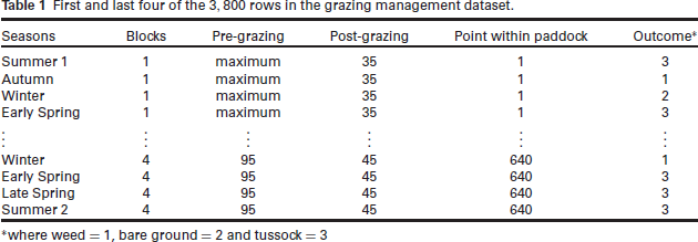
First and last four of the 3,800 rows in the grazing management dataset.
* where weed = 1, bare ground = 2 and tussock = 3
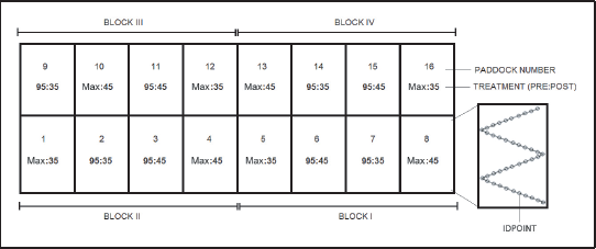
Sketch of the design of the grazing management experiment. Each of the four blocks consists of four paddocks, each one with a combination of the levels of two treatment factors. Forty points were observed within each paddock.
Here, we briefly present the main concepts to formulate the combined model for nominal outcomes. In Section 3.1, we introduce the exponential family, generalized linear models and overdispersion. In Section 3.2, we present some properties of generalized linear mixed models and the general framework of combined models.
Generalized linear models and overdispersion
The class of generalized linear models (GLM) was introduced by Nelder and Wedderburn (1972) as a framework for handling a range of common statistical models for Gaussian and non-Gaussian data. A GLM is defined in terms of three components.
The first component is a set of independent random variables, 
where 
Thus, the mean and variance of these distributions are related through

with
The second component, called linear predictor or natural parameter,
The multinomial distribution is a natural starting point for analysis of polytomous outcomes. This distribution arises as a natural extension of the binomial distribution when each independent trial has more than two possible mutually exclusive outcomes. Consider a series of 
We can safely reduce the dimensionality of 
where
It is well known that (3.3) implies a restrictive variance function. According to Grunwald et al. (2011) and Demétrio et al. (2014), cases where the variance is greater than the mean are largely reported in the literature as overdispersion, which may occur due to the absence of relevant covariates, heterogeneity of sampling units, correlation induced by hierarchical structures and/or excess of zeros. It should be noted that underdispersion can occur as well (for instance, see Ribeiro Jr et al. (2020) and Morris and Sellers (2022) for extended approaches recently developed that can be used to accommodate underdispersion). Thus, it is important to adapt models to take into account deviations from assumed mean-variance relationships in order to avoid incorrect inferences (Hinde and Demétrio, 1998).
One possibility to extend the multinomial model to handle overdispersion is to multiply the multinomial covariance matrix by a constant scalar parameter. A quasi-likelihood approach using a scale adjustment was presented by McCullagh and Nelder (1983), and later extended by Morel and Koehler (1995) to allow for different levels of overdispersion for each category using a diagonal matrix of overdispersion parameters and a Cholesky decomposition of the multinomial variancecovariance matrix. A mixture of distributions can also be used to allow for overdispersion, such as the random-clumped multinomial distribution proposed by Morel and Nagaraj (1993) and Neerchal and Morel (1998). This model is a finite mixture of multinomial distributions that captures the extra-variability caused by clumped sampling. Another convenient route to take overdispersion into account is through a two-stage approach, which considers a probability distribution for a model parameter, yielding a mixture. For instance, a multinomial model where the parameter
When analysing non-Gaussian data that are hierarchically organized (repeated measures or clustering, for example), the generalized linear mixed model (GLMM) is a popular choice (Molen-berghs and Verbeke, 2005; Diggle et al., 2002). In full generality, one assumes that, conditionally on 
where
For nominal data, it is assumed that the outcome 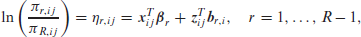

where 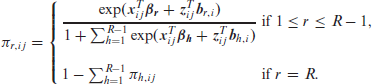
Estimates of 
The key problem in maximizing (3.5) is the presence of
While GLMMs, defined to accommodate within-unit correlation, also capture overdispersion to some extent, a single set of random effects may be insufficient to flexibly capture both. This led Molenberghs et al. (2007) to formulate a flexible and unified modelling framework, which they termed the combined model. These authors brought together two sets of random effects: the normally distributed subject-specific random effects to capture correlation and a certain amount of overdispersion, and a conjugate measurement-specific random effect on the natural parameter scale to accommodate the remaining overdispersion. Integrating out these two sets of random effects and using the generalized linear model framework, the following general family is introduced:

with notation similar to the one used in (3.4), but now with conditional mean

where
The relationship between the mean and the natural parameter is now given by the function 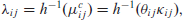
We can still apply standard GLM ideas to derive the mean and variance, combined with iterated expectation-based calculations. For the mean, if 
Molenberghs et al. (2010) and Molenberghs et al. (2017) derived explicit expressions for the means, variances, and marginal densities for a number of outcome types, such as Gaussian, Poisson, and time-to-event data. This is not possible for binary data modelled with a logit link and including Gaussian random effects, whether or not other random effects are present.
Analogously to Ivanova et al. (2014), we use a baseline-category logit structure (3.5) and include Gaussian random effects 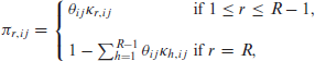
and

where
Molenberghs et al. (2007) and Molenberghs et al. (2010) showed that fitting the combined model is relatively easy, and that standard software tools can be used for maximum likelihood estimation in this case. A priori, fitting a combined model of the type described in Section 4 is done by maximizing the log-likelihood while integrating over the random effects. The joint distribution of the 
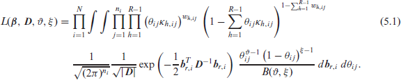
and the likelihood function can be written as:

For our proposed model, the three functions in the integrand are, in order, the multinomial, normal and beta distributions probability density or mass functions, which yields:
The key problem in maximizing (5.1) is the presence of 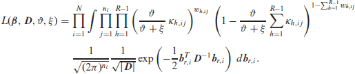
Here, a generic maximum likelihood routine that allows for integration over normal random effects can be used. We follow this route and use the SAS procedure NLMIXED. We opted for the adaptive Gaussian quadrature method (Molenberghs and Verbeke, 2005) and chose the number of quadrature points
A simulation study was conducted to compare the performance of a GLMM and the proposed combined model. We simulated longitudinal nominal data with 
where 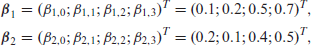
Finally, the random effects were specified as:
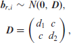
with
We simulated 200 datasets with
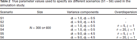
True parameter values used to specify six different scenarios (S1 - S6) used in the simulation study.
True parameter values used to specify six different scenarios (S1 - S6) used in the simulation study.
To generate data with overdispersion, the simulated probabilities were multiplied by values generated from a beta distribution with the shape parameters specified to 'strongly'
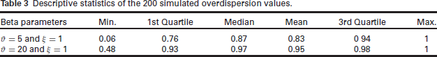
Descriptive statistics of the 200 simulated overdispersion values.
The GLMM and CM were fitted to the simulated datasets using the estimation method described in Section 5, which was implemented using SAS procedure NLMIXED. We approximated the integrals using adaptive Gaussian quadrature with 10 quadrature points, and optimized the loglikelihood using the quasi-Newton BFGS method. We used, as starting values for the fixed effects, the estimates obtained by fitting a GLM without random effects. For each scenario, we computed the average estimate (AE), bias, and mean squared error (MSE) for each parameter. We set
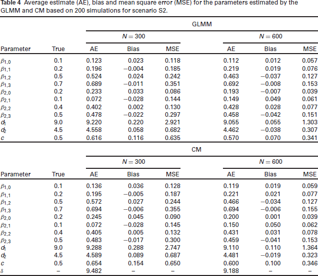
In general, the simulation results indicate the estimation procedure produced reliable results, showing that the MSEs of the maximum likelihood estimators of the parameters decay towards zero as the sample size increases, as expected under standard asymptotic theory. For scenarios S1, S2, and S4 (weak overdispersion and/or correlation), the results for both the GLMM and CM are similar (see Table 4, which displays results for scenario
Average estimate (AE), bias and mean square error (MSE) for the parameters estimated by the GLMM and CM based on 200 simulations for scenario S2.
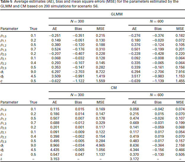
However, if there is a pronounced overdispersion effect (S3) or if it coincides with high correlations (S5 and S6), better performances were observed for the CM, mainly for the variance components (Table 5 displays results for scenario S6). Even with a larger sample size, the predicted random effects for the CM showed smaller bias and MSE when compared to the GLMM.
Average estimates (AE), bias and mean square errors (MSE) for the parameters estimated by the GLMM and CM based on 200 simulations for scenario S6.
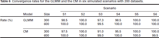
We present the convergence rates for the two models when 200 datasets were simulated in Table 6. The proportion of datasets for which convergence was achieved is a little bit smaller in the CM than in the GLMM. This can be attributed to sensitivity to the starting values, which points to the need for careful selection. When convergence problems arise, we suggest to start the analysis with the GLM or GLMM estimates and, if necessary, to attempt to fit the CM using different sets of starting values.
Convergence rates for the GLMM and the CM in six simulated scenarios with 200 datasets.
For a particular application that a researcher envisages, it might be useful to conduct a targeted simulation study to assess the convergence rate for a sample size that is envisaged.
Here, we present an analysis of the grazing management data, introduced in Section 3.2. This dataset has been previously analysed by Menarin and Lara (2017), through extended generalized estimating equations that use local odds ratios to explain the dependence among the categories (Touloumis et al., 2013). Here, emphasis was placed on a subject-specific interpretation. Let 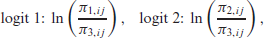
where
We then performed backwards selection for the fixed effects, by fitting reduced models which did not include higher-order interactions, and carrying out likelihood-ratio tests until the model only included significant interactions and/or main effects. This process yielded the following linear predictor:
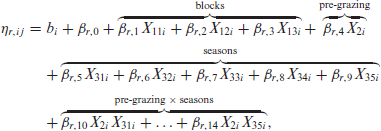
where
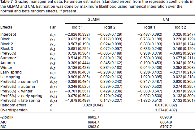
The results of both fitted models are presented in Table 7. The estimates are very similar, but there is a reduction in the variance component for the
Grazing management data. Parameter estimates (standard errors) from the regression coefficients in the GLMM and CM. Estimation was done by maximum likelihood using numerical integration over the normal and beta random effects, if present.
Grazing management data. Parameter estimates (standard errors) from the regression coefficients in the GLMM and CM. Estimation was done by maximum likelihood using numerical integration over the normal and beta random effects, if present.
To compare the models, the likelihood-ratio test was used. The difference between deviances is 11.8; however, since this test is carried out on the boundary of the parametric space, the reference distribution is a mixture of
Note that, when using the GEE approach in Menarin and Lara (2017), evidence of significant post-grazing management effect was reported, while here neither the GLMM nor CM confirmed this effect. For this experiment, overdispersion is likely to happen since it is a field experiment that can suffer from several environmental changes, and also because some types of vegetation can occur in an aggregate pattern inside paddocks.
In this article, we have proposed a model for overdispersed, repeated nominal data. The model combines the baseline-category logit assumption to handle the nominal nature of the outcome, with normal random effects in the linear predictor to deal with correlation across repeated measures, and beta random effects to flexibly account for overdispersion. Similar models were proposed by Molenberghs et al. (2007), Molenberghs et al. (2010), Molenberghs et al. (2012), Ivanova et al. (2014), and Molenberghs et al. (2017) for count data, binary and binomial data, time-to-event and ordinal outcomes. The model is easy to formulate and can be fitted using, for example, the SAS procedure NLMIXED.
A simulation study was conducted to examine the behaviour of the combined model relative to the more conventional GLMM. Both models performed well, but when there is a pronounced effect of overdispersion, or if the overdispersion effect is associated with high correlations between the repeated measurements, better performance was observed for the CM, mainly for the variance components.
We applied the GLMM and the CM to agricultural experimental data to model the probability of occurrence of three types of vegetation. Comparing both models, evidence is found in favour of the CM. It means that besides the parameter to take into account the correlation between measures, an extra overdispersion parameter was useful to accommodate the extra-variability induced by the environmental and biological changes.
Appendix A: Algebraic developments for the CM
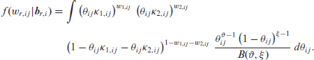
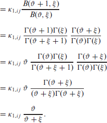
The partially marginalized density function of the combined model was obtained by integrating analytically over the beta random effects, leaving the normal random effects untouched. To do this, we need to consider the category to which the outcome belongs in order to proceed with the integration over the beta random effect. To simplify notation, let us consider the case where three categories are analysed. We can rewrite this expression as
Thus, if the outcome belongs to the first category, that is, 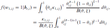
Similar results apply to r = 2, but multiplied, of course, by their respective κ. For the last category 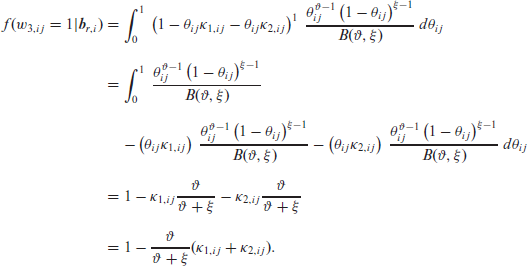
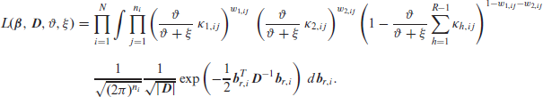
Hence, the partially marginalized likelihood function of the combined model considering three categories is given by:
Supplementary materials
Supplementary materials for this article is available online.
Supplemental Material for A combined overdispersed longitudinal model for nominal data by Ricardo K. Sercundes, Geert Molenberghs, Geert Verbeke, Clarice G.B. Demétrio, Sila C. da Silva, and Rafael A. Moral, in Statistical Modelling
Footnotes
Declaration of Conflicting Interests
The authors declared no potential conflicts of interest with respect to the research, authorship and/or publication of this article.
Funding
RKS was supported by CAPES and CNPq (proc. no. 233554/2014-9), Brazil. CGBD and SCS were supported by CNPq, Brazil.
References
Supplementary Material
Please find the following supplemental material available below.
For Open Access articles published under a Creative Commons License, all supplemental material carries the same license as the article it is associated with.
For non-Open Access articles published, all supplemental material carries a non-exclusive license, and permission requests for re-use of supplemental material or any part of supplemental material shall be sent directly to the copyright owner as specified in the copyright notice associated with the article.