
Abstract
Actuaries have long been interested in the forecasting of mortality for the purpose of the pricing and reserving of pensions and annuities. Most models of mortality in age and year of death, and often year of birth, are not identifiable so actuaries worried about what constraints should be used to give sensible estimates of the age and year of death parameters, and, if required, the year of birth parameters. These parameters were then forecast with an ARIMA model to give the required forecasts of mortality. A recent article showed that, while the fitted parameters were not identifiable, both the fitted and forecast mortalities were. This result holds if the age term is smoothed with P-splines. The present article deals with generalized linear models with a rank deficient regression matrix. We have two aims. First, we investigate the effect that different constraints have on the estimated regression coefficients. We show that it is possible to fit the model under different constraints in R without imposing any explicit constraints. R does all the necessary booking-keeping ‘under the bonnet’. The estimated regression coefficients under a particular set of constraints can then be recovered from the invariant fitted values. We have a black box approach to fitting the model subject to any set of constraints.
Introduction
Actuaries have long been interested in the forecasting of human mortality for the purpose of the pricing and reserving of pensions and annuities. Gompertz (1825), in a landmark paper, gave the first mathematical model of mortality. He only had death rates by age at ten year intervals but he observed that these rates were linear on a log scale. This enabled him to interpolate for all ages for the range of ages he had available. This was the celebrated Gompertz law of mortality.
At the present time extensive mortality data are available not only by single ages but also by year of death. The Human Mortality Database is a comprehensive resource of mortality data and gives mortality data (a) by age and year of death in a calendar year, and (b) an estimate of the mid-year number of lives exposed to the risk of death in that year. These data are available on over 40 countries for the male and female populations of these countries.
These richer datasets gave rise to the possibility not only of modelling mortality by age and year but also the forecasting of mortality. Such models were in terms of age and year of death, and often year of birth. The idea was to estimate the parameters in the models and then forecast the year of death parameters and, if required, the year of birth parameters; see Cairns et al. (2009) for a comprehensive treatment of such models. However, there was a problem—most models were not identifiable so it was not obvious how to obtain parameter estimates that would give sensible forecasts. Various sets of linear constraints on the parameters were proposed that would solve this problem.
Most models were generalized linear models or GLMs. Currie (2020) showed that, while the fitted parameters were not identifiable, the fitted mortalities were identifiable (a fundamental result in regression modelling) but crucially the forecast values of mortality were also identifiable when forecasting was done with an ARIMA model. This article illustrated this result by considering two sets of constraints, one a standard set of constraints found in the literature (see Cairns et al., 2009, for example) and the other a set of random constraints. A general proof of the result was also provided.
The purpose of the present article is twofold: first, to show that we can ignore the explicit use of constraints completely and use R’s
We do not present any general theory but rather present our method through a single model, the Age-Period-Cohort model. We consider this model in a basic form and also in a smooth form where we use P-splines (Eilers an Marx 1996) to smooth some terms in the model. It should be clear that our method applies more generally.
Data and notation
We illustrate our ideas with data from the Human Mortality Database on UK males (data downloaded February 2022). We adopt the convention that matrices are denoted by upper case bold font as in
In addition, the following notation is useful:
The Age-Period-Cohort model
Let
The Age-Period-Cohort or APC model is the simplest model which involves the age and year of death, and the year of birth. We define

where

where
The usual actuarial approach is to choose three suitable constraints and then forecast the resulting estimates of
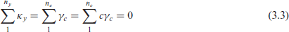
see Cairns et al. (2009). We refer to (3.3) as the standard constraints. We can fit the APC model in R with the


Inspection of
What is the connection between the approach to identifiability used by R and that often used by actuaries? We can mimic R’s method with the constraints

ie, we constrain the final period parameter and the final two cohort parameters to be zero. We refer to these constraints, implicit in R’s approach, as the R constraints. We refit the APC model with the constraints (3.7). Currie (2013) gave the following generalization of the GLM scoring algorithm to fit a GLM with constraints

Here
We have fitted the model without the need to specify constraints. If we wish for some reason to find a fit with specified constraints we proceed as follows. We seek a solution of the GLM scoring algorithm

Let
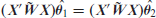

Now

This expression exists in another form which is particularly illuminating. We observe that

In other words, we can compute the estimated coefficients subject to any particular set of constraints directly from the invariant fitted values. Invariance is a fundamental and powerful idea and (11) demonstrates just one result from applying it.
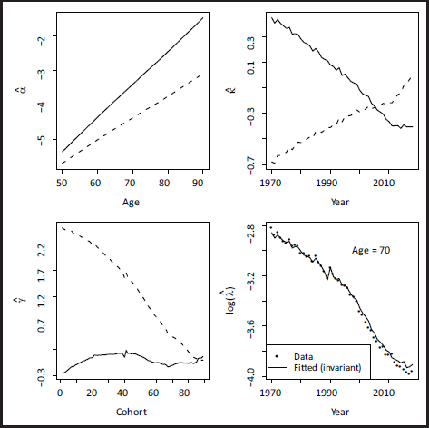
Figure 1 emphasizes the effect that constraints can have on parameter estimates. The effect on the estimates of the time parameters is particularly striking. Under the standard constraints one may be tempted to interpret the parameter estimates as indicating improving mortality. The estimates under the R constraints indicate exactly the opposite. What can be said is that mortality does improve over time but that can only be concluded securely from the invariant fitted mortality shown in the lower right panel.
Estimates of
,
and
under standard constraints (solid line), R constraints (dashed line) and the observed and invariant fitted log mortality for age 70.
We examine the differences in the parameter estimates. We define


for some constants A, B and C. We conclude that the three sets of differences are linearly related with slopes C, -C and C. With our data and the standard and R constraints we found A=-1.163 B=1.465 and C=0.03199. Despite appearances to the contrary in Figure 1 the two sets of estimates are intimately related.
Gompertz smoothed the age parameters with a simple linear function. Here we use the method of P-splines to smooth the age parameters,
Let

where

for a GLM with Poisson errors and a log link.
We could use a generalization of (3.8) where the upper left block becomes
We can avoid the use of algorithms like (3.8) with data augmentation; see Eilers and Marx (2021), p35. Data augmentation enables us to fit the smooth APC model with code similar to (3.4), (3.5) and (3.6) for the original APC model discussed in section 3. We define the augmented model matrix and augmented working variable as follows:

It follows immediately that

Thus solutions of the penalized scoring algorithm (4.1) and

are equal. Equation (4.5) is weighted least squares so we can fit the model with R’s
We choose
We use the following extension of (3.11)

to investigate the relation between the two sets of estimates obtained under the standard and R constraints. We put
As in the unsmoothed case, we define
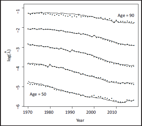
Figure 2 shows the observed and fitted log mortalities for age 50 to 90 at ten year intervals. Evidently, there has been a steady improvement in mortality over the observation period. This improvement corresponds to an approximate increase in life expectancy of two years every ten years. For example, life expectancy in the UK in 1970 was 72.3 years and this has risen to 81.2 years in 2019. This has major consequences for the provision of both state and private pensions.
Observed and fitted log
for ages 50 to 90 at ten year intervals for the smooth APC model.
This short article has highlighted the effect that different constraint systems can have on parameter estimates. Figure 1 is a dramatic example of such effects. We have also highlighted the role of the invariant fitted values. Equation (3.11) shows that knowledge of these invariant values yields parameter estimates under any particular constraint system. We have used the basic
Footnotes
Acknowledgements
I am grateful for the invitation to submit an article for this special issue. I met Brian on many occasions: it would be hard to imagine anyone with a greater zest for life in general and statistics in particular. I am also grateful for his great paper with Paul Eilers which introduced the world to P-splines. It has dominated my working life for over twenty years. I would also like to thank Paul Eilers for his encouragement to write this short article.
Declaration of Conflicting Interests
The author declared no potential conflicts of interest with respect to the research, authorship and/or publication of this article.
Funding
The author received no financial support for the research, authorship and/or publication of this article.