
Abstract
A new approach to represent P-splines as a mixed model is presented. The corresponding matrices are sparse allowing the new approach can find the optimal values of the penalty parameters in a computationally efficient manner. Whereas the new mixed model P-splines formulation is similar to the original P-splines, a key difference is that the fixed effects are modelled explicitly, and extra constraints are added to the random part of the model. An important feature ensuring that the entire computation is fast is a sparse implementation of the Automated Differentiation of the Cholesky algorithm. It is shown by means of two examples that the new approach is fast compared to existing methods. The methodology has been implemented in the R-package LMMsolver available on CRAN (
Introduction
Penalized regression using B-splines (known as P-splines; Eilers and Marx, 1996, 2021) is computationally efficient, because of the local character of B-splines. The corresponding linear equations are sparse and can be solved quickly. However, the main problem is to find the optimal value for the tuning or penalty parameter. A good way to approach this problem is to use mixed models and restricted maximum likelihood (REML; Patterson and Thompson, 1971). Several methods have been proposed to transform the original P-spline model to a mixed model (Eilers, 1999; Currie and Durban, 2002; Lee and Durbán, 2011). A disadvantage of existing transformations to mixed models is that the local character of the B-splines is lost, which reduces computational efficiency.
The proposed transformations have in common that they start from the P-splines formulation and decompose into a fixed and a random term to obtain a mixed model. The same idea can be used for tensor product P-splines (Currie et al., 2006; Lee and Durbán, 2011; Lee et al., 2013; Rodríguez-Ávarez et al., 2015; 2018; Wood et al., 2013; Wood, 2017). There are many different ways to represent tensor product P-splines as a mixed model; Piepho et al. (2022) give an overview of the different two-dimensional P-splines models.
Here, a new and efficient approach is outlined. In Boer et al., (2020) it was shown that the linear variance (LV) mixed model (Williams, 1986) is equivalent to P-splines with first-degree B-splines and first-order differences. This idea will be generalized here, to show that P-splines with
Another property of the LV model is that it is computationally attractive, as the precision matrix is sparse. It will be shown that the P-splines model is equivalent to a class of mixed models with a sparse precision matrix. In this article we will show that the sparse mixed model P-splines are computationally efficient.
The layout of the article is as follows. In Section 2 we will discuss in detail the equivalence between the linear variance mixed model and a special case of P-splines. Section 3 outlines a brief overview of B-splines, and gives some results that will be used to derive the connection between mixed models and P-splines. In Section 4 it will be shown how the idea presented in Section 2 can be generalized to P-splines. Section 5 shows how this can be further extended to mixed model tensor product P-splines. In Section 6 an implementation of the sparse mixed model in the
Linear variance model and Whittaker smoother
The Whittaker smoother (Whittaker, 1923) and the Linear Variance (LV) mixed model introduced by Williams (1986) are equivalent, as shown by Boer et al. (2020). Here we will use a new approach to show that the two models are equivalent with the aim to develop a computational efficient method to estimate the optimal penalty parameters using mixed models that can be further extended to P-splines. The Whittaker smoother is a special case of P-splines (Frasso and Eilers, 2015), and originally third-order differences were used by Whittaker (1923). Here we will use a simpler variant of Whittakers proposal, using first-order differences.
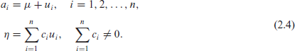
Suppose there are

where

where
In this article we will formulate mixed models in terms of penalty and precision matrix (the inverse of the covariance matrix), which is a more modern representation (Lindgren et al., 2022). The parameter

where
To make the connection between the LV model and the Whittaker smoother, we define the following invertible linear transformation:
Using equation (2.4) and

we obtain

Equation (2.6) can be decomposed as

and
The LV and the RW mixed models have a sparse precision matrix and they can be solved in a computational efficient way (Boer et al., 2020). This approach can be further extended to show that there are mixed models, with sparse precision matrices, that are equivalent to P-splines. The method can be generalized to tensor product P-splines, as shown in Section 5.
In this section we will give a brief overview of B-splines; for more details see for example De Boor (1978) and Lyche et al. (2018). Let the domain

where
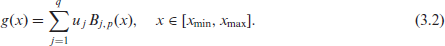
The

where
Let

where

a result that will be used to establish, in Sections 4 and 5, the equivalence of a class of mixed models with P-splines.
The idea of representing polynomials in terms of B-splines can be extended a bit further, and this idea will be used to derive our main result in Section 4. Suppose we are interested in the interpolating

Let
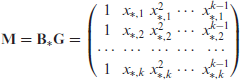
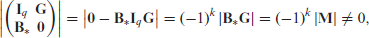
with determinant (Harville, 1998, section 13.6)

The determinant is unequal to zero, since the points
Using the B-splines properties described in the previous section, we can generalize the results from Section 2 to P-splines. First we introduce some notation. Let
In the next step we will define a model equivalent with P-splines, following the same steps as in Section 2. To make this connection more clear, we will use the same subscripts for the objective functions to be minimized, cf. equations (2.3), (2.6), and (2.7). The objective function

where

with
where we use the properties of block matrices in the first step (Harville, 1998, section 13.3), and equation (3.7) in the second and third steps. For the differences we have

using
By substitution of equation (4.2) into equation (4.1) and using equation (4.3) we obtain

Equation (4.4) can be decomposed as

is the objective function to be minimized for P-splines (Eilers and Marx, 1996), and
In this section we will extend the new formulation of P-splines to higher dimensions. We generalise the notation that was used for the one-dimensional case. Let
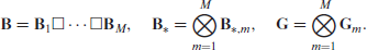
The fixed part of the model is given by
For the product between
using that
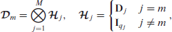
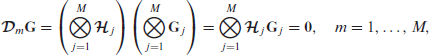
Define the tensor product objective function

Using the linear transformation defined in equation (4.2) and

we obtain

Since
This shows that equations (5.1) and (5.3) are equivalent. In Section 6 we will present an efficient mixed model formulation of equation (5.1). Rodríguez-Ávarez et al. (2015) use another transformation of tensor P-splines to a mixed model, which is based on the spectral decomposition of the difference penalty matrices
The
Solving the linear mixed equations
The penalized regression model defined by equation (5.1) can be formulated as a mixed model:

with

where

The matrix on the left hand side of equation (6.3) is called the mixed model coefficient matrix and will be denoted by
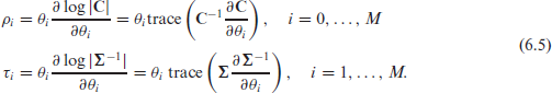
The followings equations are used to update the precision parameters
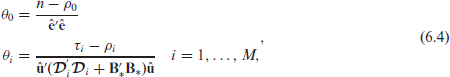
where
The iterative algorithm defined by equations (6.3) and (6.5) is an extension of the modified Henderson algorithm described in Harville (1977).
An important element needed is to calculate
In this section we will compare the performance of
All computations were performed in R4.2.3 (R Core Team 2023) and a 2.90GHz Intel Core i5-9400 CPU with 24GB of RAM and Windows10 operating system. Version 1.8.42 of
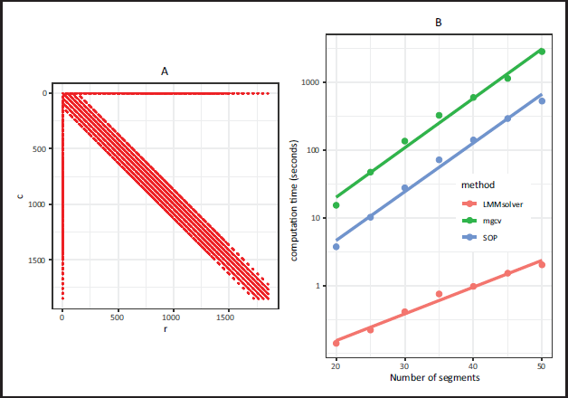
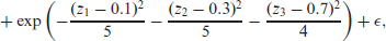
Figure 1A shows the sparse structure for the mixed model coefficient matrix corresponding to equation (5.1) for
Panel A: The mixed model coefficient matrix
for the new approach for the US precipitation example with
segments for both latitude and longitude. The non-zeros are indicated in red, showing that
is sparse. Panel B: Computation time on a logarithmic scale for the three methods as function of the number of segments in both dimensions: LMMsolver is much faster, especially if the number of segments is high.
In Figure 1B the computation time is compared for different number of segments, showing that
There are two main reasons why
In this section we will use a simulated three-dimensional example to illustrate that
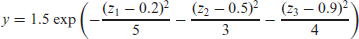
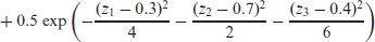
with
Discussion
In this article we have shown that there is a mixed model formulation for P-splines that adheres closely to the original proposal by Eilers and Marx (1996). The main difference is that in the new approach there is an explicit term for the fixed part, with an additional term for the penalty. An important feature is that the precision matrices and the mixed model equations are sparse. Therefore the sparse matrix algebra developed for mixed models can be used.
An additional advantage of the new approach is that the mixed model P-splines formulation can be further extended to Generalized Additive Models (GAM; Hastie et al., 2009). In standard P-splines a small ridge penalty is added to make the system identifiable (Eilers and Marx, 2021). In the approach described here, this problem does not arise: the column corresponding to
The mixed model P-splines formulation extends the P-splines framework developed by Paul Eilers and Brian Marx (1996, 2021). An interesting aspect of the mixed model P-splines formulation is that it takes advantage of the properties of the two key components of P-splines: B-splines and discrete difference penalties.
Panel A: The mixed model coefficient matrix
for the new approach for the three-dimensional simulated data with
segments for each dimension. The non-zeros are indicated in red. Panel B: Computation time on a logarithmic scale for LMMsolver , mgcv, and SOP as function of the number of segments in each dimension.
Appendix A
In this appendix we will give a derivation of equation (6.4). The restricted log-likelihood of equation (6.1) is given by (Meyer and Smith, 1996):

where

and therefore equation (A.1) can be rewritten as:

with matrices
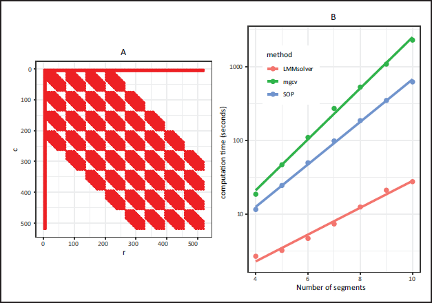
The partial derivatives of equation (A.3) are given by
where the parameters
Setting the partial derivatives in equation (A.4) equal to zero gives the expressions for
Supplementary materials
Supplementary materials for this article are available online.
Supplemental Material for Tensor product P-splines using a sparse mixed model formulation by Martin P. Boer, in Statistical Modelling
Footnotes
Acknowledgements
I would like to thank Bart-Jan van Rossum for his contribution to the
Declaration of Conflicting Interests
The author declared no potential conflicts of interest with respect to the research, authorship and/or publication of this article.
Funding
The author received no financial support for the research, authorship and/or publication of this article.
References
Supplementary Material
Please find the following supplemental material available below.
For Open Access articles published under a Creative Commons License, all supplemental material carries the same license as the article it is associated with.
For non-Open Access articles published, all supplemental material carries a non-exclusive license, and permission requests for re-use of supplemental material or any part of supplemental material shall be sent directly to the copyright owner as specified in the copyright notice associated with the article.