
Abstract
A truncated, mean-parameterized Conway-Maxwell-Poisson model is developed to handle under- and overdispersed count data owing to individual heterogeneity. The truncated nature of the data allows for a more direct implementation of the model than is utilized in previous work without too much computational burden. The model is applied to a large dataset of Test match cricket bowlers, where the data are in the form of small counts and range in time from 1877 to the modern day, leading to the inclusion of temporal effects to account for fundamental changes to the sport and society. Rankings of sportsmen and women based on a statistical model are often handicapped by the popularity of inappropriate traditional metrics, which are found to be flawed measures in this instance. Inferences are made using a Bayesian approach by deploying a Markov Chain Monte Carlo algorithm to obtain parameter estimates and to extract the innate ability of individual players. The model offers a good fit and indicates that there is merit in a more sophisticated measure for ranking and assessing Test match bowlers.
Introduction
Statistical research in cricket has been somewhat overlooked in the stampede to model football and baseball. Moreover, the research that has been done on cricket has largely focused on batsmen, whether modelling individual, partnership and team scores (Kimber and Hansford, 1993, Scarf et al., 2011; Pollard et al., 1977), or ranking Test batsmen (Brown, 2009, Rohde 2011; Boys and Philipson, 2019; Stevenson and Brewer, 2021), or on short-format cricket via predicting match outcomes (Davis et al., 2015) or optimising the batting strategy in one day and Twenty20 international cricket (Preston and Thomas, 2000; Swartz et al., 2006; Perera et al., 2016). Indeed, to the author’s knowledge, this is the first work that explicitly focuses on Test match bowlers.
Test cricket is the oldest form of cricket. With a rich and storied history, it is typically held up as being the ultimate challenge of ability, nerve and concentration, hence the origin of the term ‘Test’ to describe the matches. For Test batsmen, their value is almost exclusively measured by how many runs they score and their career batting average, with passing mention made of the rate at which they score, if this is remarkable. Test bowlers are also primarily rated on their (bowling) average, which in order to be on the same scale as the batting average is measured as runs conceded per wicket, rather than the more natural rate of wickets per run. In this work we consider the problem of comparing Test bowlers across the entire span of Test cricket from its genesis in March 1877 to the modern day, July 2022.
Rather uniquely, the best bowling averages of all-time belong to bowlers who played more than a hundred years ago, contrast this with almost any other modern sport where records are routinely broken by current participants, with their coteries of support staff dedicated to fitness, nutrition and wellbeing along with access to detailed databases highlighting their strengths and weaknesses. The proposed model allows us to question whether the best Test bowlers are truly those who played in the late 19th and early 20th century or whether this is simply a reflection of the sport at the time. Along the way, we also deliberate whether the classic bowling average is the most suitable measure of career performance. Taking these two aspects together suggests that there are more suitable alternatives than simply ranking all players over time based on their bowling average, as seen at
The structure of the article is as follows. The data are described in Section 2 and contain truncated, small counts which, at the player level, are both under and overdispersed, leading to the statistical model in Section 3. Section 4 details the prior distribution alongside the computational details. Section 5 presents some of the results and the article concludes with some discussion and avenues for future work in Section 6.
The data
The data used in this article consists of N = 47 216 individual innings bowling figures by n = 2 207 Test match bowlers from the first Test played in 1877 up to Test 2 473, in July 2022. There are currently twelve Test playing countries and far more Test matches are played today than at the genesis of Test cricket (Boys and Philipson, 2019). World Series Cricket matches are not included in the dataset since these matches are not considered official Test matches by the International Cricket Council (ICC).
Bowling data for a player on a cricket scorecard comes in the form ‘overs-maidens-wickets-runs’—note that in this work the first two values provide meta-information that are not used for analysis—as seen at the bottom of Figure 1. A concrete example are the bowling data for James Anderson with figures of 25.5-5-61-2. The main aspect of this to note is that the data are aggregated counts for bowlers—2 wickets were taken for 61 runs in this instance, but it is not known how many runs were conceded for each individual wicket. This aggregation is compounded across all matches to give a career bowling average for a particular player, corresponding to the average number of runs they concede per wicket taken. This measure is of a form that is understandable to fans, but counter-intuitive from the standpoint of a statistical model; this point is revisited in subsection 3.1.1.
Bowling figures as seen on a typical cricket scorecard.
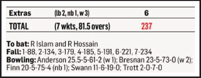
Bowling figures as seen on a typical cricket scorecard.
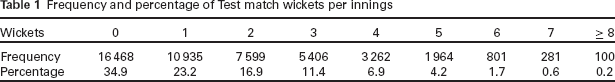
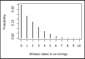
In each Test match innings there are a maximum of ten wickets that can be taken by the bowling team, and these wickets are typically shared amongst the team’s bowlers, of which there are nominally four or five. Table 1 shows the distribution of wickets taken in an innings across all bowlers, with Figure 2 providing a visual representation. Taking six wickets or more in an innings is rare and the most common outcome is that of no wickets taken.
Frequency and percentage of Test match wickets per innings
Probability mass function of Test match wickets taken per innings.
Alongside the wickets and runs, there are data available for the identity of the player, the opposition, the venue (home or away), the match innings, the winners of the toss and the date the match took place. These are all considered as covariates in the model.
To motivate the model introduced in section 3, the raw indices of dispersion at the player level show that around 20% of players have underdispersed counts, approximately 20% of players have equidispersed counts, with the remainder having overdispersed counts. This overlooks the effects of covariates but suggests that any candidate distribution ought to be capable of handling both under- and overdispersion, or bidispersion at the player level.
Wickets taken in an innings are counts and a typical, natural starting point may be to consider modelling them via the Poisson or negative binomial distributions. However, in light of the bidispersion seen at the player level in the raw data, we instead turn to a distribution capable of handling such data.
The Conway-Maxwell-Poisson (CMP) distribution (Conway and Maxwell, 1962) is a generalization of the Poisson distribution, which includes an extra parameter to account for possible over- and underdispersion. Despite being introduced almost sixty years ago to tackle a queueing problem, it has little footprint in the statistical literature, although it has gained some traction in the last fifteen years or so with applications to household consumer purchasing traits (Boatwright et al., 2003), retail sales, lengths of Hungarian words (Shmueli et al., 2005), and road traffic accident data (Lord et al., 2008, 2010). Its wider applicability was demonstrated by Guikema and Goffelt (2008) and Sellers and Shmueli (2010), who recast the CMP distribution in the generalized linear modelling framework for both Bayesian and frequentist settings respectively, and through the development of an R package (Sellers et al., 2019) in the case of the latter, to help facilitate routine use.
In the context considered here, the CMP distribution is particularly appealing as it allows for both over- and underdispersion for individual players. For the cricket bowling data, we define 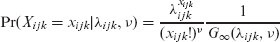
with
Sellers et al., (2019) implemented the CMP model using a closed-form approximation (Shmueli et al., 2005; Gillispie and Green, 2015) when
Truncated mean-parameterized CMP distribution
The standard CMP model is not parameterized through its mean, however, restricting its wider applicability in regression settings since this renders effects hard to quantify, other than as a general increase or decrease. To counter this, two alternative parameterizations via the mean have been developed (Huang, 2017; Ribeiro Jr et al., 2018; Huang and Kim, 2019), each with associated R packages (Fung et al., 2019; Elias Ribeiro Junior, 2021). The mean of the standard CMP distribution can be found as
which, upon rearranging, leads to
Hence, the CMP distribution can be mean-parameterized to allow a more conventional count regression interpretation, where
Irrespective of mean parameterization and method, the above model formulation has two obvious flaws: the counts lie on a restricted range, that is, 0, ..., 10, and there is no account taken of how many runs the bowler conceded in order to take their wickets. For the first issue, the model can be easily modified using truncation, which, in this case, leads to a simplified form for the CMP distribution, which is exploited below:
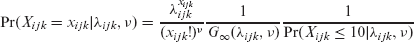
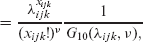
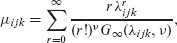
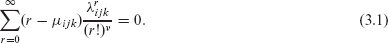
where 
Since
As noted earlier, data are only available in an aggregated form. That is, the total number of wickets is recorded alongside the total number of runs conceded. Historically, this has been converted to a cricket bowling average by taking the rate of runs conceded to wickets taken, chiefly to map this on to a similar scale as to the classic batting average. However, in the usual (and statistical) view of a rate this is more naturally expressed as wickets per run, rather than runs per wicket, and this rate formulation is adopted henceforth. In either event, the number of runs conceded conveys important information since taking three wickets at the cost of thirty runs is very different to taking the same number of wickets for, say, ninety runs.
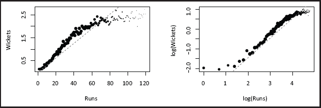
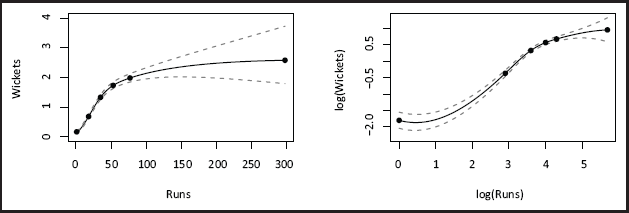
By looking at the mean number of wickets for each value of runs the relationship between wickets and runs can be assessed, see Figure 3; note that there is very little data for values of runs exceeding 120 so the plot is truncated at this point. The nonlinear relationship rules out instinctive choices such as an offset or additive relationship—this makes sense as the number of wickets taken by a bowler cannot exceed ten in a (within-match) innings, which suggests that the effect of runs on wickets is unlikely to be wholly multiplicative (or additive on the log-scale).
Average wickets taken for values of runs on the linear (left) and log (right) scales. The size of the data points reflects the amount of data for each value of runs; the dashed line represents the relationship under the traditional cricket bowling average.
Average wickets taken for values of runs on the linear (left) and log (right) scales. The size of the data points reflects the amount of data for each value of runs; the dashed line represents the relationship under the traditional cricket bowling average.
Smoothing splines in the form of cubic B-splines are adopted to capture the nonlinear relationship, with knots chosen at the quintiles of runs (on the log scale). This corresponds to internal knots at 18, 35, 53 and 77 along with the boundary knots at 1 and 298 on the runs scale. Various nonlinear models were also considered but did not capture the relationship as well as the proposed spline.
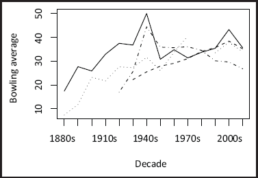
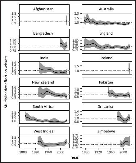
As the data span 146 years it is perhaps unreasonable to assume that some effects are constant over time. In particular, teams are likely to have had periods of strength and/or weakness whereas conditions, game focus, advances in equipment and technology may have drastically altered playing conditions for all teams at various points in the Test cricket timeline. A plot of the mean bowling average across decades for a selection of opposition countries is given in Figure 4. Here we use the conventional bowling average on the y-axis for ease of interpreation, but the story is similar when using the rate. Clearly, the averages vary substantially over time as countries go through periods of strength and weakness and game conditions and rules evolve. As such, treating them as time invariant effects does not seem appropriate. Note also that some countries started playing Test cricket much later than 1877 (see the lines for West Indies and India in Figure 4) and teams appear to take several years to adapt and improve.
Mean bowling averages across decades for a selection of opposing countries: Australia (solid line), India (dashed), South Africa (dotted) and West Indies (dot-dash).
Mean bowling averages across decades for a selection of opposing countries: Australia (solid line), India (dashed), South Africa (dotted) and West Indies (dot-dash).
This motivates the inclusion of dynamic opposition effects, where we again adopt smoothing splines, this time with knots chosen at the midpoints of decades (of which there are fourteen); this is a natural timespan, both in a general and sporting sense; cricket followers will often discuss the West Indies of the 1980s or Australia of the 1990s for instance. For identifiability, the opposition effect of Australia in 2022 is chosen as the reference value.
As well as runs conceded by a bowler and the strength of opposition, there are several other factors that can affect performance, some of which are considered formally in the model. Introducing some notation for available information:
These remaining terms in the model for the wicket-taking rate are assumed to be additive and, hence, the mean log-rate is modelled as
where
The design matrices
For identifiability purposes we set
CMP regression also allows a model for the dispersion. Here, recognizing that we may have both under and overdispersion at play, we opt for a player-specific dispersion term
R (R Core Team, 2022) was used for all model fitting, analysis and plotting, with the
For analysis, four MCMC chains were run in parallel with 1 000 warm-up iterations followed by 5 000 further iterations. Model fits took approximately eight hours on a standard MacBook Pro. A Metropolis-within-Gibbs algorithm is used in the MCMC scheme, with component-wise updates for all parameters except for those involved in the spline for runs, β. For these parameters a block update was used to circumvent the poor mixing seen when deploying one-at-a-time updates, with the proposal covariance matrix based on the estimated parameter covariance matrix from a frequentist fit using the
Prior distribution
For the innings, playing away and winning the toss effects we use zero mean normal distributions with standard deviation 0.25, reflecting a belief that these effects are likely to be quite small on the multiplicative wicket-taking scale, with effects larger than 50% increases or decreases deemed unlikely (with a 5% chance a priori). The same prior distribution is used for the player ability terms,
For the dispersion parameters we work on the log-scale, introducing
Results
Functional form for runs
A plot of wickets against runs using the posterior means for
Mean wickets taken against runs on the linear (left) and log (right) scales with 95% HDI interval uncertainty bands; solid circles represent the knots for the spline.
Mean wickets taken against runs on the linear (left) and log (right) scales with 95% HDI interval uncertainty bands; solid circles represent the knots for the spline.
A plot of the fitted posterior mean profiles for each opposition is given in Figure 6. The largest values of all occur for South Africa when they first played (against the more experienced England and Australia exclusively); most teams struggle when they first play Test cricket, as shown by the largest posterior means at the left-hand side of each individual plot (since we are modelling the rate, which is the inverse of the traditional average). Overall, this led to the low Test bowling averages of the 1880s-1900s that still stand today as the lowest of all-time and adjusting for this seems fundamental to a fairer comparison and/or ranking of players.
Posterior mean and 95% HDI bands for each opposition.
Posterior mean and 95% HDI bands for each opposition.
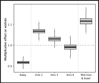
The posterior means and 95% highest density intervals (HDIs) for the innings effects—on the multiplicative scale—are 1.07 (1.04–1.09), 1.03 (1.01–1.06) and 0.99 (0.96–1.02) for the second, third and fourth innings respectively, when compared to the first innings. Similarly, the effect of playing away is to reduce the mean number of wickets taken by around
Boxplots of the posterior distributions for playing away (
), match innings 2–4 (
) and winning the toss and bowling (
)
Boxplots of the posterior distributions for playing away (
), match innings 2–4 (
) and winning the toss and bowling (
)
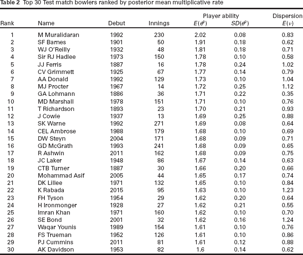
The top thirty bowlers, as ranked by their posterior mean ability,
Top 30 Test match bowlers ranked by posterior mean multiplicative rate
Top 30 Test match bowlers ranked by posterior mean multiplicative rate
The rankings under the proposed model differ substantially from a ranking based on bowling average alone. As a case in point, the lowest, that is, best, bowling average of all time belongs to GA Lohmann, who is ranked 9th in our model. Similarly, Muttiah Muralidaran, who tops our list, is 50th on the list of best averages at the time of writing. The main ramifications of using the proposed model is that players from the early years are ranked lower, and spinners are generally ranked higher. The latter is an artefact of the model, in that bowling long spells and taking wickets is now appropriately captured through the nonlinear effect for runs.
We also see from Table 2 that five players—all seam bowlers interestingly—have underdispersed data judging from the posterior means of
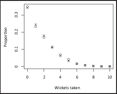
The performance of the model is evaluated using the posterior predictive distribution. Namely, due to the small number of observed counts, it is viable to compare the model-based posterior predictive probability for each observed value of 0, 1, ..., 10 and compare that to the observed probability in each case. A summary of this information is given in Figure 8, where we see excellent agreement between the observed and expected proportions at each value of wickets.
Observed (grey circles) and model-based (crosses) probabilities for each value of wickets.
Observed (grey circles) and model-based (crosses) probabilities for each value of wickets.
The outcome of interest considered here was the number of wickets taken by a bowler in an innings, which was modelled using a truncated mean-parameterized Conway-Maxwell-Poisson distribution. The model allows for comparisons between players from different eras through the inclusion of dynamic opposition effects alongside axiomatic game-specific effects of home advantage, pitch conditions and the best use thereof. However, there are other factors that were not considered here, principally due to the aggregated nature of the data, which precludes looking at the ability of bowlers to break partnerships, take top-order wickets or to perform at their best in the most important matches, in their most crucial stages.
Other classic count models were considered, but it was found that Poisson and negative binomial regression models failed to adequately describe the data. Alternative count models capable of handling both under- and overdispersion may perform equally well, such as those based on the gamma count, generalized Poisson, double Poisson or Poisson-Tweedie distributions, although each of these has some limitations. Looking further afield, an exponentially tilted multinomial model (Rathouz and Gao, 2009) may offer increased flexibility over the aforementioned count data models. Alternative models are not pursued further here, owing to the good performance of the chosen model and the nontrivial implementation of such non-standard models (that would require bespoke coding) in this big data setting.
Additional metrics not formally modelled here are bowling strike rate and bowling economy rate, which concern the number of balls bowled (rather than the number of runs conceded) per wicket and runs conceded per over respectively. Whilst both informative measures, they are typically viewed as secondary and tertiary respectively to bowling average in Test cricket, where time is less constrained than in shorter form cricket. Hence, future work looking at one day international or Twenty20 cricket could consider the triple of average, strike rate and economy rate for bowlers, alongside average and strike rate for batsmen, thereby requiring a multivariate count data model.
One limitation of this work is that we have ignored possible dependence between players, the taking of wickets can be thought of as a competing resource problem and the success (or lack of) for one player may have an impact on other players on the same team. Indeed, the problem could potentially be recast as one of competing risks. However, this argument is rather circular in that a bowler would not concede many runs if a teammate is taking lots of wickets and this is taken into account through the modelling of the relationship between wickets and runs.
The MPCMP model may have broader use in other sports where there may be bidispersed data, for example modelling goals scored in football matches—stronger and weaker teams are likely to exhibit underdispersion; hockey, ice-hockey and baseball all have small (albeit not truncated) counts as outcomes of interest with bidispersion likely at the team or player level, or both. Moving away from sports to other fields, the MPCMP model could be used to model parity, which is known to vary widely across countries with heavy underdispersion (Barakat, 2016), or scores in the popular web-based word game, Wordle. It could also be appropriate for longitudinal counts with volatile (overdispersed) and stable (underdispersed) profiles at the patient level, where the level of variability may be related to a clinical outcome of interest in a joint modelling setting. Indeed, it will have broader use in any field where counts are subject to bidispersion.
This work has shown that truncated counts subject to bidispersion at some hierarchical level can be handled in a mean-parameterized CMP model, based on a large dataset, without too much computational overhead. Further methodological work is needed to implement the model in the case of non-truncated counts and to seek faster computational methods.
Footnotes
Acknowledgements
Thanks to the late Professor Richard Boys, this work is dedicated in memory of him. The genesis of this work was a Masters project under his kind supervision farther back in time than I would care to remember.
Further thanks to the reviewer and editor whose comments helped improve the article and provided some thought-provoking content to help shape future research.
Declaration of Conflicting Interests
The author declared no potential conflicts of interest with respect to the research, authorship and/or publication of this article.
Funding
The author received no financial support for the research, authorship and/or publication of this article.