
Abstract
Spatial smoothing makes use of spatial information to obtain better estimates in regression models. In particular flexible smoothing with B-splines and penalties, which has been propagated by Eilers and Marx (1996), provides strong tools that can be used to include available spatial information. We consider alternative smoothing methods in spatial additive regression and employ them for analysing rental data in Munich. The first method applies tensor product P-splines to the geolocation of apartments, measured on a continuous scale through the centroid of the quarter where an apartment is. The alternative approach exploits the neighbourhood structure of districts on a discrete scale, where districts consist of a set of neighbouring quarters. The discrete modelling approach yields smooth estimates when using ridge-type penalties but can also enforce spatial clustering of districts with a homogeneous structure when using Lasso-type penalties.
Introduction
According to German Law, increases in rents for apartments can be justified on ‘average rents’ for apartments that are comparable in size, location, equipment and quality. Such average rents are thereby published in official rental guides (Mietspiegel). Munich and most other larger cities publish rental guides, usually based on regression models with net rent or net rent per square meter as the dependent variable and characteristics of the apartment as explanatory variables. The models are based on data from surveys and are an official instrument in the German apartment rental market (see e.g., Fahrmeir et al., 1995 or Fitzenberger and Fuchs, 2017). Resulting rental guides appear in form of tables that are easy to use for both tenants and landlords. Therefore, suitable regression models should provide good predictive performance but should not be unnecessarily complex. A general discussion of statistical aspects in rental guides in Germany can be found in Kauermann and Windmann (2016).
Statistical consulting and analyses for rental guides for the city of Munich are carried out by the Department of Statistics, LMU Munich, since 1992. Coincidentally, this is the year when the first version of P-splines was presented by Eilers and Marx (1992) at the GLIM and Statistical Modelling Meeting in Munich. The use of P-spline for rental guides however occurred much later, after the seminal publication of Eilers and Marx (1996), for modelling the distinctly non-linear effect of size (in square meters) of an apartment—and possibly also of the year of construction—on its net rent per square meter. The inclusion of categorical variables characterizing equipment and quality then leads to additive regression models. Given that the data are available for research, they have been used as example in many further papers, including for instance Fahrmeir et al. (1998), Stasinopoulos et al. (2000), Kneib (2013) or De Bastiani et al. (2018).
It is well known that the location of an apartment has high predictive value, but suitable inclusion and modelling of this important spatial variable is non-trivial. The current Munich rental guide contains two types of location variables. First, as a categorical variable obtained from expert assessment in combination with exploratory statistical analysis. This variable describes the local neighbourhood, which is categorized into the average, high, and top residential areas. Additionally, the location of the apartment is also included in the rental guide, categorized into central and non-central locations. We refer to the webpage mietspiegel-muenchen.de for an exact definition. While the first variable describes the quality of the local residential area, the second variable refers to the spatial location within the city borders of Munich. The combination of the two discrete variables leads to 6 (= 2 × 3) categories referring to location.
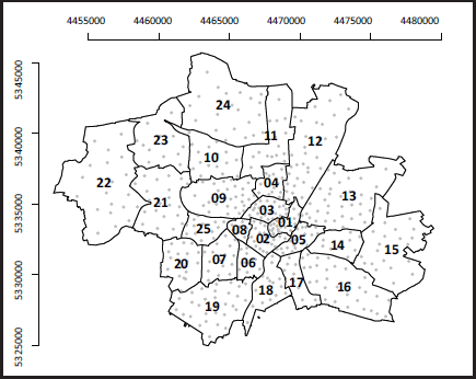
In this article we focus on the influence of the location of the apartment in a rigorous data-based manner, utilizing more detailed information from the data. That is we aim at extending the currently used rental guide. For reasons of data protection, the exact address of an apartment is not provided, but the city of Munich is divided into 475 quarters. For each apartment, we know the quarter the apartment is located in. Calculating the centroid for each quarter will allow for spatial smoothing by substituting the exact location of the apartment through the corresponding quarter centroid. The quarters themselves are grouped into 25 districts as a coarser categorization. We will also propose to use the districts and the resulting neighbourhood structure of the districts for smoothing as well as spatial clustering. Both, the centroids of quarters and the 25 districts are visualized in Figure 1.
Map of districts 1 to 25 and centroids of quarters in Munich with coordinates.
Map of districts 1 to 25 and centroids of quarters in Munich with coordinates.
We focus on spatial additive regression models, also called geoadditive models (Kammann and Wand, 2003), evaluating and comparing different but related forms of spatial smoothing. Bivariate and spatial smoothing for continuous and discrete spatial variables is described, for example, in Fahrmeir et al. (2021), covering tensor product P-splines, kriging, thin plate splines, radial basis function and Markov random field approaches. For P-spline smoothing in one or more dimensions we refer to the very readable surveys of Eilers et al. (2015) and Eilers and Marx (1992). Smoothing on lattice data, in particular, its contrasts to spatial econometrics, is discussed in Kauermann et al. (2012).
The article is organized as follows. In Section 3, we use centroids as continuous spatial variable and apply tensor product P-splines for estimating a smooth spatial effect. In Section 4, we use the districts as discrete spatial variable and smoothing methods based on lattice data. Section 4.2 considers lattice smoothing using a Ridge-type penalty, derived from Gaussian Markov random fields for the effects of neighbouring districts. In Section 4.3, we replace this smoothing penalty with a Lasso-type penalty, enforcing spatial clustering through a selection of neighbouring districts with differences of effects close to or equal to zero. We also consider the identification of clusters of neighbouring districts with (approximately) the same spatial effects, which is a sensible goal to formulate rental guides that are easier to interpret and communicate. Though our comparison of the three versions of spatial smoothing is illustrated and motivated by application to the Munich rental guide data, we are convinced that this comparison will be rather useful for many other fields of application, for example, in epidemiology or labour market research.
We analyse data from the 2019 Munich rental guide. The data were collected through a survey where the sample was drawn from the residential registration office. The survey was carried out through personal or video-based interviews. Only apartments were included that fulfilled particular legal criteria, which are of no particular interest to the application given here. All in all, we have data on 3 255 apartments. As response variable
Explanatory variables included in the models with rent as response variable.
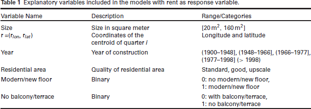
Explanatory variables included in the models with rent as response variable.
Smooth spatial additive regression
We assume the net rent per square meter to follow a spatial, additive regression model of the form

where 
where
The smooth functions can be estimated by P-splines, as originally introduced by Eilers and Marx (1992) in a first version and in the well-known article of Eilers and Marx (1996). The method gained massive interest in the last 25 years and we refer to Eilers et al. (2015) or Eilers and Marx (2021) for survey work. We do not give many technical details here but refer to the comprehensive survey work cited above. Instead, we want to focus on the idea of penalization and do this in the spatial context for the estimation of function
To estimate
First, a two-dimensional B-spline basis is constructed on the convex hull of the spatial locations 
consisting of all pairs of univariate B-splines in the longitudinal and latitudinal directions. Here, 
where 
where 
with 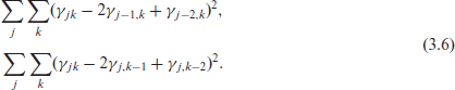
These ridge-type penalties (3.6) for the location effect can be expressed as

where the penalty matrix 
Smoothing parameters can be estimated via the
Estimated effect
for every quarter.
We show the fitted spatial effect in Figure 2, where one can clearly see that the centre part of Munich has higher apartment rents which get smaller with more distance from the city centre. It is also seen that the decrease in rent in the north/south direction is less visible than in the east/west direction. This can be explained by the topology of Munich, with the river Isar running from south to north through Munich, and proximity to the river is mirrored in higher apartment rents.
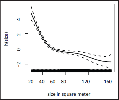
The effect of apartment size is visualized in Figure 3. We see a decreasing effect but generally not a complicated structure of the function. In the remainder of the article, we will therefore model this effect with a six-dimensional quadratic B-spline basis and omit the penalty on the coefficients
Estimates, standard error and resulting standardized values resulting from the P-Spline model.
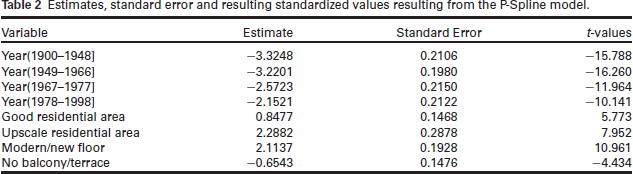
Estimates, standard error and resulting standardized values resulting from the P-Spline model.
Effect of apartment size in P-Spline smoothing.
Lattice data
As already discussed, the geolocation used for each apartment in the previous section is not its exact longitude and latitude coordinates, but the centroid of the corresponding quarter so that spatial smoothing as proposed above is carried out over a finite set of distinct centroids. For practical purposes, this is still burdensome when applying the rental guide, due to a large number of quarters in Munich. It is therefore easier to coarsen the spatial variable and work with districts instead of quarters. We visualized the step from quarters to districts already in Figure 1. In this case, centroids of districts are less useful to work with, since there are only 25 distinct values. We now consider the district to correspond to a lattice with a neighbour structure, as visualized in Figure 1. This opens a new avenue of spatial smoothing by taking the lattice structure as spatial information instead of the Euclidean distance between the district centroids. We, therefore, use the following neighbourhood structure and numerate the districts from
Note that smoothing on lattice data ignores the Euclidean distance. In spatial smoothing, as carried out in the previous section, we imposed through the penalty (3.5), that apartments lying close together have a similar rent level. In lattice smoothing, instead, it is only postulated that neighbouring districts have similar rent levels, regardless of their Euclidean distance. While in general, it sounds less plausible for smoothing to rely on lattice data if coordinates are available, it does make sense for rental guide data. First, districts themselves have some homogeneity regardless of their size. This is ignored in spatial smoothing but implicitly taken into account in lattice smoothing. Second, in terms of applicability, it is far easier to give a general rent level per district instead of per geolocation or quarter.
Lattice smoothing with ridge-type penalties
We consider again model (3.1), but now 
We define 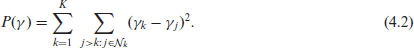
The penalty consists of squared differences of all possible combinations of neighbouring districts, where each combination is considered only once. This yields a penalty that discourages large deviations of effects associated with neighbouring regions. The penalty can also be derived from the Gaussian Markov random field approach, see Fahrmeir et al. (2021, Section 8.2.4).
Let the 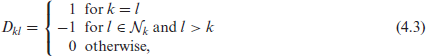
where 
where
By setting 
with 
The penalty (4.5) then has the form

yielding as simple squared regularization. As remarked in Section 3, the non-linear effect of the apartment size is fitted by a simple six-dimensional quadratic B-spline and the remaining covariates are included in the model as before. This leads to the penalized L2 loss which we aim to minimize

where matrix
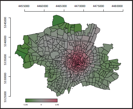
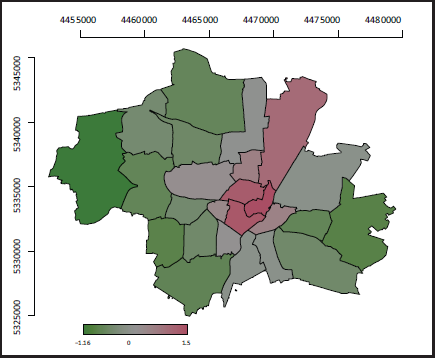
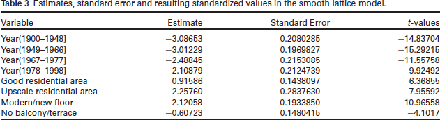
The corresponding smooth district effect is shown in Figure 4. The resulting effects for the covariates are given in Table 3. The effect of size is not visualized as this looks very much like the penalized fit shown in Figure 3. Generally, Table 3 shows comparable results to Table 2, hence changing the spatial model has only a small impact on the categorical covariates. Looking at Figure 4 we see little variation in the eastern and western suburbs of Munich, which already appeared from Figure 2. We may therefore question, whether some neighbouring districts in fact have the same rent level. This is further examined in the next modelling step.
Estimated effect
for every quarter
Eimates, standard error and resulting standardized values in the smooth lattice model.
The penalty (4.7) corresponds to simple ridge regression, that is, we impose an L2 component on the coefficients. An alternative is to proceed with LASSO estimation, that is, replacing the L2 with L1. We, therefore, postulate that the difference between neighboring districts should be small in absolute terms, that is,
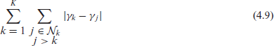
which can be rewritten as 
for different values of the penalty parameter
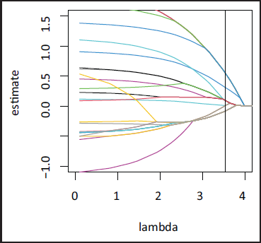
In Figure 5 we show the estimates for parameters
Generalized Lasso estimates for different penalization parameters. The vertical line shows the model with the smallest BIC.
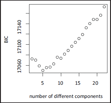
BIC for different models. The number of components corresponds to the number of splits resulting for different values of
in Figure 5.
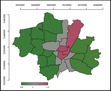
Estimated effects
after Lasso model selection.
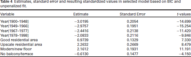
Estimates, standard error and resulting standardized values in selected model based on BIC and unpenalized fit.
In this article, we considered three different versions of smoothing applied to the Munich rental data. We used smoothing based on geolocations of apartments, grouped to centroids of quarters. We also grouped the quarters into districts and considered these as lattice, penalized by both, an L2 as well as an L1 loss.
At least in our application, the estimates of other covariate effects are quite robust with respect to the different versions of smoothing. Therefore, the choice of a specific spatial model will be guided by the specific goals of smoothing. While P-spline smoothing for quarters is well-suited for providing a refined global picture of spatial effects, Lasso-type smoothing for districts with automated spatial clustering is very useful for developing applicable rental guides.
We chose to run this comparison with data from Munich to remember Brian Marx’s many visits to our home town. Beyond working on statistical modelling and giving lectures at the Department of Statistics, LMU Munich, Brian enjoyed good things in life together with us, such as hiking or biking along the banks of the river Isar, visiting beergardens in and around Munich, and having fun with friends. Although this article focuses on spatial smoothing for rental guides, spatial clustering as in Section 4.3. can be of interest in many other applications. This motivates further methodological research: In its current version, the generalized Lasso is restricted to linear models with an additional spatial component. It might be useful or even necessary, to allow for Ridge-type penalties, as for P-splines, in combination with generalized Lasso penalties. The resulting optimization problem is challenging. However, We see three possible approaches: First, an alternating optimization algorithm, switching between optimizing the Ridge component for fixed parameters of the Lasso component, and vice versa, see Ohishi et al. (2019) for a grouped Lasso part and a generalized Lasso part. Second, approximation of the Lasso penalty through a differentiable function, see Oelker and Tutz (2017). Third, a Bayesian approach based on the Bayesian Lasso, with a conditionally Gaussian prior, along the lines of Masuda and Inoue (2022).
Supplementary Material
Supplemental material for this article is available online.
Supplemental Material for Spatial smoothing revisited: An application to rental data in Munich by Ludwig Fahrmeir, Göran Kauermann, Gerhard Tutz and Michael Windmann, in Statistical Modelling
Footnotes
Acknowledgment
The second author acknowledges the support of the Munich Center for Machine Learning (MCML).
Declaration of Conflicting Interests
The authors declared no potential conflicts of interest with respect to the research, authorship and/or publication of this article.
Funding
The authors received no financial support for the research, authorship and/or publication of this article.
References
Supplementary Material
Please find the following supplemental material available below.
For Open Access articles published under a Creative Commons License, all supplemental material carries the same license as the article it is associated with.
For non-Open Access articles published, all supplemental material carries a non-exclusive license, and permission requests for re-use of supplemental material or any part of supplemental material shall be sent directly to the copyright owner as specified in the copyright notice associated with the article.