A multilevel analysis of real estate valuation using distributional and quantile regression

Abstract

Real estate valuation is typically based on hedonic regression models where the expected price of a property is explained in dependence of its attributes. However, investors in the housing market are equally interested in the distribution of real estate market values (including price variation), that is, determining the impact of attributes of a property on the entire conditional distribution. We therefore consider Bayesian structured additive distributional and quantile regression models for real estate valuation. In the first approach, each parameter of a potentially complex parametric response distribution is related to a structured additive predictor. In contrast, the second approach proceeds differently and models arbitrary quantiles of the response distribution directly and nonparametrically. Both models presented are based on a multilevel version of structured additive regression thereby utilizing the typical hierarchical structure of real estate data. We demonstrate the proposed methodology within a detailed case study based on more than 3 000 owner-occupied single family homes in Austria, discuss interpretation of the resulting effect estimates, and compare models based on their predictive ability.

1 Introduction

According to Rosen (1974), a standard concept for real estate valuation is the hedonic approach, assuming that a property can be characterized by a bundle of covariates that involves both individual attributes of the building itself and regional attributes of the area the building is located in. Each of these attributes can be assigned an implicit price, summing up to the value of the entire property, see for example, Malpezzi (2003). Hedonic price theory then suggests the use of regression models that explain the price in dependence of all attributes. The functional form of this dependence should allow for non-linearities, see for example, Malpezzi (2003), Brunauer et al. (2010). Thus, we draw on generalized structured additive regression (STAR) models (Fahrmeir et al., 2004, 2022) and in particular rely on P(enalized)-splines for nonlinear effects as originally proposed by Eilers and Marx (1996), see also Eilers and Marx (2010); Eilers et al. (2015); Eilers and Marx (2021) for more recent treatments of P-splines.

In general, investors are not only interested in the expectation of house prices but also in the range of the price variation in order to evaluate the uncertainty of real estate market values, which is essential for investment decisions in individual properties or real estate portfolios. Furthermore, due to the importance of properties as collateral, fluctuations in real estate market values may have a great effect on the soundness of the financial system as a whole (see e.g., Goodhart and Hofmann, 2007). As a consequence, there is an increasing focus in the recent literature on quantiles of house prices. McMillen (2008), for example, analyses appreciation rates for different house price segments using linear quantile regression introduced by Koenker and Bassett (1978). Fritsch et al. (2016) use a semiparametric quantile regression approach in order to estimate submarket-specific hedonic price surfaces with a particular focus on spatial effects that they model as triograms of longitude and latitude.

The purpose of this article is to analyse not only the expectation of the distribution of real estate market values as a function of explanatory variables but also more general distributional features using modern regression models that overcome the focus on conditional expectations. Therefore, we apply Bayesian structured additive distributional regression models, developed in Klein et al. (2014, 2015), as well as Bayesian quantile regression (Waldmann et al., 2013) for precise estimation of the conditional distribution of house prices in dependence of covariates. In structured additive distributional regression, each parameter (and not only the mean) of a parametric response distribution is related to a (hierarchical) structured additive predictor. Semiparametric quantile regression, in contrast, models arbitrary quantiles of the response distribution directly through the structured additive predictors.

The two approaches are compared in a case study, focussing on the interpretation of resulting estimates but also considering predictive ability. For the case study, we use a dataset that has been collected by the UniCredit Bank Austria AG between October 1997 and September 2009 and contains data on 3 231 owner-occupied single-family homes in Austria, leading to $n=38772$ observations. The dependent variable in our analysis is the house price per square meter ( $p_{qm}$ ). Section A of the Supplement provides a description and summary statistics of all available variables. We estimate multilevel STAR regression models (Lang et al., 2014) thereby utilizing the hierarchical structure of the Austrian political–administrative units: Single-family homes (level-1) belong to municipalities (level-2), which are nested in districts (level-3), which are themselves nested in counties (level-4). An extensive review of the current state-of-the-art in multilevel models is provided in Scott et al. (2013).

The remainder of the article is as follows: Section 2 presents an exposition of Bayesian distributional and quantile regression models in the context of hedonic regression for house prices. Section 3 is devoted to the case study. The final section concludes and discusses directions for future research.

2 Multilevel Distributional and Quantile Regression

2.1 Assumptions on the response distribution

In distributional regression, following the idea of generalized additive models for location, scale and shape (Stasinopoulos et al. 2021), we rely on parametric distributional specifications for the response variable, that is, the conditional distribution of the responses $y_i$ given covariates is assumed to be characterized by a parametric density $p(y_i|$ ${}_i)$ with $L$ -dimensional parameter vector ${}_i=({\vartheta }_{i1}\mathrm{,}\dots \mathrm{,}{\vartheta }_{iL}{)}^{\prime }$ . Similar as in generalized additive models, each of these parameters is then related to a corresponding regression predictor via bijective response functions such that ${\vartheta }_{il}=h_l({\eta }_{il})$ , $l=1,\dots \mathrm{,}L$ , ensuring appropriate restrictions on the parameter spaces.

A wide variety of distributions with different characteristics is available in distributional regression, see Klein et al. (2015); Stasinopoulos et al. (2021) for overviews. In the context of our application, we rely on the Gaussian distribution with only the mean being a function of covariates while the variance is homoscedastic (Gaussian), a heteroscedastic Gaussian model where both the mean and the variance are functions of covariates (HetGaussian), the same models but with log-transformed responses (Loggaussian, HetLoggaussian) and the gamma distribution in the mean/scale parameterization typically assumed in generalized linear and additive models with both mean and scale parameter being functions of covariates (Gamma). While the Gaussian model assumes a symmetric distribution for house prices, the log-normal and gamma models pick up the stylized feature of positively skewed prices as well as the restriction to positive prices.

Rather than relying on a specific type of distribution, quantile regression as introduced by Koenker and Bassett (1978) focuses on modelling specific quantiles of the response distribution directly. For a given quantile level $\phi \in (\mathrm{0,1})$ , estimation in linear quantile regression relies on minimizing the asymmetrically weighted error (AWE) criterion

$${\displaystyle \sum _{i=1}^n}{\rho }_{\phi }(y_i-{\eta }_{i\phi }),\hspace{1em}with\hspace{1em}{\rho }_{\phi }(u)=\left\{\begin{array}{cc}u\phi & ifu\ge 0\\ u(\phi -1)& ifu<\mathrm{0,}\end{array}\right.$$

(2.1)

and quantile-dependent linear predictor ${\eta }_{i\phi }=$ x ${}_{i^{\prime }}$ ${}_{\phi }$ . One can then show that the $\phi$ -quantile of the conditional response distribution is given by the minimizer ${\widehat{\eta }}_{i\phi }$ of this loss function. Since there exists no closed form solution for this minimization problem, estimates are typically obtained based on linear programming and modifications of the simplex algorithm (see Koenker and D’Orey, 1987; Koenker, 2005, for details). The distribution of the response can then be approximated by the estimated quantiles $q_{\phi }$ provided that the quantiles are estimated for a reasonably dense grid of $\phi$ -values.

Generalizations of quantile regression allowing for structured additive predictors are conceptually straightforward but estimation is highly challenging and almost impossible for more complex models. We therefore resort to Bayesian quantile regression that relies on an auxiliary likelihood approach that provides the same point estimates as frequentist quantile regression. Following Yue and Rue 2011), we assume independent and identically distributed observations following an asymmetric Laplace distribution (ALD) with location parameter ${\eta }_{i\phi }$ , scale parameter ${\sigma }^2$ and skewness parameter $\phi$ , that is, $y_i|{\eta }_{i\mathrm{,}\phi }\mathrm{,}{\sigma }^2\mathrm{,}\phi \stackrel{iid}{\sim }ALD({\eta }_{i\phi }\mathrm{,}{\sigma }^2\mathrm{,}\phi )$ with density

$$p(y_i|{\eta }_{i\phi }\mathrm{,}{\sigma }^2\mathrm{,}\phi )=\frac{\phi (1-\phi )}{{\sigma }^2}\exp \left(-\frac{{\rho }_{\phi }(y_i-{\eta }_{i\phi })}{{\sigma }^2}\right)\mathrm{.}$$

Maximizing the corresponding posterior (for fixed ${\sigma }^2$ and $\phi$ ) obviously is equivalent to minimizing the AWE criterion (2.1). Since the check function ${\rho }_{\phi }$ is non-differentiable, inference based on Markov chain Monte Carlo (MCMC) simulations at a first glance seems to be complicated. However, the asymmetric Laplace distribution can be represented as a location scale mixture of normals such that simple Gibbs steps can be utilized, see Yue and Rue (2011) and Waldmann et al. (2013) for details.

2.2 Basic predictor and prior

In all our models, the basic predictor (dropping the distributional parameter index $l$ and the quantile level $\phi$ ) is of the form

$${\eta }_i=f_1(z_{i1})+\dots +f_q(z_{iq})+{\text{x}}_{i^{\prime }}\gamma \mathrm{,} i=1,\dots \mathrm{,}n\mathrm{,}$$

where the functions $f_j$ comprise nonlinear effects of the continuous covariates $z_{ij}$ (e.g., the floor area, the age of the building, the year of purchase) or indicate a spatial index of the region a certain observation belongs to (e.g., municipality, district or county) while the term $x_i^{\prime }\gamma$ includes the categorical covariates. Dropping the function index $j$ , any functional effect $f$ can be approximated by

$$f(z)={\displaystyle \sum _{k=1}^K}{\beta }_k{B}_k(z)\mathrm{,}$$

where $B_1\mathrm{,}\dots \mathrm{,}{B}_K$ is a set of $K$ known basis functions and $\beta =({\beta }_1,\dots ,{\beta }_K{)}^{\prime }$ being a vector of unknown regression coefficients to be estimated. Defining the $n\times K$ design matrix $Z$ with elements $Z[i\mathrm{,}k]=B_k(z_i)$ , the vector $f=(f(z_1),\dots ,f(z_n){)}^{\prime }$ of function evaluations can be written in matrix notation as $\mathbf{f}=Z\beta$ . Accordingly, for observed data we obtain the generic predictor representation

$$\eta ={\text{Z}}_1{\beta }_1+\dots +{\text{Z}}_q{\beta }_q+\text{X}\gamma \mathrm{.}$$

To prevent overfitting and to enforce desirable properties of the estimates we assume (possibly improper) Gaussian priors of the form

$$p(\beta |{\tau }^2)\propto {\left(\frac{1}{{\tau }^2}\right)}^{ rk \left(\text{K}\right)/2}\exp \left(-\frac{1}{2{\tau }^2}\beta \text{'}\text{K}\beta \right)\cdot I(\text{A}\beta =\text{0})\mathrm{,}$$

(2)

where $I(\cdot )$ is the indicator function. The key components of the prior are the penalty matrix K , the variance parameter ${\tau }^2$ and the constraint $\mathbf{A}\mathbf{\beta }=\mathbf{0}$ . Usually the penalty matrix is rank deficient, that is, $rk ($ K $)<K$ , resulting in a partially improper prior. The specific structure of K depends on the covariate type and on prior assumptions about the smoothness of $f$ . The term $I(A\beta =0)$ imposes required identifiability constraints on the parameter vector. A straightforward choice is $A=(1,\dots ,1)$ , that is, the regression coefficients are centered around zero. The amount of smoothness is governed by the variance parameter ${\tau }^2$ . A conjugate inverse Gamma prior is employed for ${\tau }^2$ , that is, ${\tau }^2\sim IG(a\mathrm{,}b)$ with small values for the hyperparameters $a$ and $b$ resulting in an uninformative prior on the log scale. As a default we choose $a=b=0.001$ . However, in order to evaluate the model’s robustness and validity we re-estimate all our models with different hyperparameter choices and compare the corresponding results (see Section C of the Supplement).

The exact choices of basis functions and prior properties encoded in the precision matrix K depend on the covariate and term type, see Fahrmeir et al. (2022) for details on various effect types. In our context, the relevant effect types are P(enalized)-splines introduced in a frequentist setting by Eilers and Marx (1996) and transferred to a Bayesian version by Lang and Brezger (2004). P-splines assume that the unknown functions can be approximated by a polynomial spline which can be written in terms of a linear combination of B-spline basis functions, while the precision matrix is determined from difference operators applied to the sequence of basis coefficients. In the frequentist approach, this implies a roughness penalty of the form $\lambda {\beta }^{\prime }K\beta$ where the smoothing parameter $\lambda$ and the variance parameter ${\tau }^2$ are connected by $\lambda =\frac{1}{{\tau }^2}$ .

2.3 Multilevel models

In a multilevel STAR model (Lang et al., 2014), the regression coefficients ${\mathbf{\beta }}_j$ of a function $f_j$ may themselves obey a regression model with a structured additive predictor, that is, ${\mathbf{\beta }}_j\sim \mathcal{N}({\eta }_j\mathrm{,}{\tau }_j^{2}I)$ with ${\eta }_j=Z_{j1}{\beta }_{j1}+\dots +Z_{j{q}_j}{\beta }_{j{q}_j}+X_j{\gamma }_j$ where the terms $Z_{j1}{\beta }_{j1}\mathrm{,}\dots \mathrm{,}{Z}_{j{q}_j}{\beta }_{j{q}_j}$ represent additional nonlinear functions $f_{j1}\mathrm{,}\dots \mathrm{,}{f}_{j{q}_j}$ , and $X_j{\gamma }_j$ comprises additional linear effects. Further levels are possible by assuming that the second level regression parameters ${\beta }_{jl}$ , $l=1,\dots \mathrm{,}{q}_j$ , again obey a STAR model.

In this article, we use the multilevel structure if a covariate $z_j\in \{1,\dots \mathrm{,}K\}$ is a spatial index and $z_{ij}$ indicates the region observation $i$ pertains to. Then, the design matrix $Z_j$ is an $n\times K$ incidence matrix with $Z_j[i\mathrm{,}k]=1$ if the $i$ -th observation belongs to region $k$ and zero otherwise. The $K\times 1$ parameter vector ${\beta }_j$ is the vector of regression parameters, that is, the $k$ -th element in ${\beta }_j$ corresponds to the regression coefficient of the $k$ -th region. The use of the compound prior above allows for further explaining the region-specific effect by spatial covariates (e.g., the purchase power index, the share of academics, etc.).

The hierarchical structure of the Austrian political–administrative units suggests the use of the following four level predictor for each distributional parameter/quantile being modeled:

$$\begin{array}{llll} level-1: \hfill & \eta \hfill & =\hfill & {\text{f}}_1(area)+{\text{f}}_2(area\_plot)+{\text{f}}_3(age)+{\text{f}}_4(time\_ind)+\hfill \\ \hfill & \hfill & \hfill & {\text{f}}_5(municipality)+\text{X}\gamma \hfill \\ level-2: \hfill & {\beta }_5\hfill & =\hfill & {\text{f}}_{\mathrm{5,1}}(pp\_ind)+{\text{f}}_{\mathrm{5,2}}(ln\_educ)+{\text{f}}_{\mathrm{5,3}}(age\_ind)+{\text{f}}_{\mathrm{5,4}}(comm)+\hfill \\ \hfill & \hfill & \hfill & {\text{f}}_{\mathrm{5,5}}(ln\_dens)+{\text{f}}_{\mathrm{5,6}}(district)+{\epsilon }_5\hfill \\ level-3: \hfill & {\beta }_{\mathrm{5,6}}\hfill & =\hfill & {\text{f}}_{\mathrm{5,6,1}}(wko\_ind)+{\text{f}}_{\mathrm{5,6,2}}^{mrf}(district)+{\text{f}}_{\mathrm{5,6,3}}(county)+{\epsilon }_{\mathrm{5,6}}\hfill \\ level-4: \hfill & {\beta }_{\mathrm{5,6,3}}\hfill & =\hfill & 1{\gamma }_0+{\epsilon }_{\mathrm{5,6,3}}.\hfill \end{array}$$

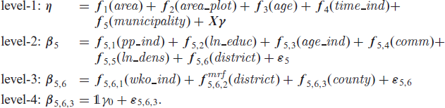
In the equations for levels 2, 3 and 4, the left hand side of the model specification $\left({\mathbf{\beta }}_5,{\mathbf{\beta }}_{5,6},{\mathbf{\beta }}_{5,6,3}\right)$ represents the vector of spatial effects from the right hand side one step up in the multilevel specification, that is, ${\mathbf{\beta }}_{\mathrm{5,6,3}}$ relates to $f_{\mathrm{5,6,3}}(county)$ , ${\mathbf{\beta }}_{\mathrm{5,6}}$ relates to $f_{\mathrm{5,6}}(district)$ , and ${\mathbf{\beta }}_5$ relates to $f_5(municipality)$ .

The level-1 equation includes the continuous variables floor area (area), plot area where the house is built on (area_plot), age of the building at the time of sale (age), calculated as the difference between the year of purchase and the year of construction, and the year of purchase (time_ind). For a detailed description of further level-1 categorical covariates see Section A in the Supplement. An uncorrelated random municipality effect $f_5(municipality)$ is further added in the level-1 equation to control for unordered spatial heterogeneity. This heterogeneity is modeled through the level-2 equation and is further decomposed into a district and finally into a county level effect (levels 3 and 4). At the municipality and the district level further covariates are observed and used in the subsequent analysis. Examples for level-2 covariates are sociodemographic and economic attributes as the purchase power index (pp_ind) and the share of academics (educ) as a proxy for the average level of education. On the district level we incorporate a real estate price index (wko_ind) reflecting the local house price level. Furthermore, district specific spatial heterogeneity is modeled through a correlated spatial effect $f_{\mathrm{5,6,2}}^{mrf}(district)$ in the level-3 equation by Markov random fields.

The multilevel specification of our model does not only relate to the different nature of the explanatory variables but also enables considerable efficiency gains for the computations. On the one hand, Gibbs steps can be considered for the updates on all higher levels of the hierarchy, leading to faster computations since no acceptance step is needed. On the other hand, we typically observe improved mixing and convergence compared to reduced form specifications, see Lang et al. (2014) for details.

3 Case Study

We now present the estimation results for the models described in Section 2. In Section 3.1, we compare four parametric response distributions for the distributional regression framework. The best-fitting distribution is then compared to quantile regression in terms of effect estimates in Section 3.2. A comparison in terms of predictive ability is provided in the supplement, Section B. All results are based on a final MCMC run with 120 000 iterations and a burn in period of 20 000 iterations for all models. We stored every 100th iteration in order to obtain a sample of 1 000 practically independent draws from the posterior, which we verified using common MCMC diagnostics, see Section C of the supplement.

3.1 Distributional regression

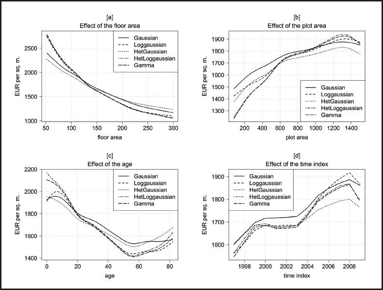
Figure 1 shows the posterior mean expected house prices per square meter as functions of the structural continuous covariates in the parametric models. In order to get an impression of the magnitude of effects and to make the results comparable, we show partial effect plots where the other covariates are fixed at ‘typical values’. For the continuous structural covariates, these typical values represent the mean level of attributes, for categorical variables the most frequent level, and for all neighborhood covariates and spatial effects we chose the covariates of the most frequent municipality. We refer to this setting as ‘evaluated at the average effect’ in the following. Since the effects are quite different in magnitude, we do not show them on the same scale.

Figure 1:

Posterior mean estimates of the expected house prices per square meter from the distributional regression models for the continuous structural level-1 covariates (evaluated at the average effect).

In panel [a], the effect of the floor area (variable area) is shown. For all models, we find a monotonically decreasing and very pronounced effect, which is in line with the law of diminishing marginal utility. The decreasing effect weakens as the floor area becomes larger. While the results of the skewed distributions (Loggaussian, HetLoggaussian and Gamma model) are virtually the same and cover a range of up to 1 730 Euro, in the Gaussian and the HetGaussian model the effect only accounts for a variation of 1 230 Euro and 1 040 Euro, respectively.

Additional plot area (area_plot, panel [b]) yields higher prices per square meter, with the effect becoming weaker as plot area increases. For very large plots, the effect even seems to reverse. However, the data only include very few observations with plot areas larger than 1 300 square meters, leading to wide credible intervals in this area (not shown in the figure). Again, the Gamma model and the HetLoggaussian model yield effects that are more pronounced compared to the other models. Here, the results of the Loggaussian model as well deviate from those of the HetLoggaussian and Gamma model, which are again very similar. In total, house prices per square meter change by about 390 Euro (Gaussian model) to 690 Euro (Gamma model and HetLoggaussian model) over the domain of the plot area.

The effect of the age of the building, shown in panel [c], can be considered as the rate of depreciation of single family homes. Thus, the initial increase up to an age of 7 years in the results of the Gaussian and the Loggaussian model seems quite unlikely, whereas the more or less linear depreciation (until an age of about 55 years) in the other models is in line with our expectations. However, the decline is much more pronounced in the HetLoggaussian and the Gamma model than in the HetGaussian model. In all models, the effect slightly reverses for old buildings (again with wide credible intervals due to a small number of observations in this area). The age of the house covers a range of about 425 Euro (Gaussian model) to 750 Euro (Gamma model) per square meter.

The effect of the time index (panel [d]) shows the quality controlled development of house prices over time. After a moderate increase from 1997 to 2000, prices almost stay constant until 2003 with similar results for almost all models. Only the Gaussian model predicts slightly higher prices in this period. After 2003 the prices rise until 2008 in a considerably different extent within the five models: While the increase is less marked for the Gaussian and the HetGaussian model, it is more pronounced especially for the Loggaussian model. In the last year of the observation period, prices consistently decrease, indicating the effect of the economic crisis of 2008/2009. In total, the time index accounts for variation in a range of 200 Euro (HetGaussian model) to 350 Euro (Loggaussian model).

The results of the spatial covariates are shown in Figure 2. The effect of the purchase power index (pp_ind), shown in panel [a], is highly positive between 80 and 130 index points with similar results for the skewed models and slightly weaker effects for the symmetric models. The negative effects for low and high values of the purchase power index are unexpected, but may result from very few municipalities with such extreme index points (wide credible intervals). In total, house prices per square meter change by about 300 Euro (Gaussian model) to 475 Euro (Gamma model).

Figure 2:

Posterior mean estimates of the expected house prices per square meter from the distributional regression models for the spatial level-2 and level-3 covariates (evaluated at the average effect).

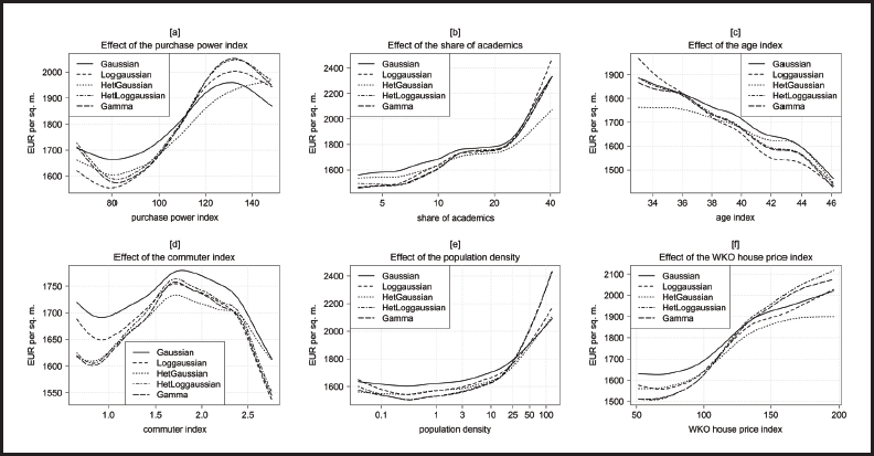
Although the share of academics (ln_educ, panel [b]) enters the equation logarithmically, it is displayed in natural values. The effect is positive, with a pronounced increase starting at a share of approximately 25%. The difference between all models is rather small, only for municipalities with a very high amount of academics the HetGaussian model seems to underestimate the effect compared to the other models. The share of academics accounts for a variation of up to 1 000 Euro (Gamma model).

The effect of the age index (age_ind, panel [c]) is more or less linear for all models with the highest slope in the Loggaussian model (bandwidth of about 535 Euro) and the smallest one in the HetGaussian model (bandwidth 320 Euro). The negative direction is in line with our expectations and can be interpreted as a decreasing attractiveness of municipalities that exhibit an excess of age.

The commuter index (comm, displayed in panel [d]) has the weakest effect of all continuous covariates with a variation of not more than 220 Euro. The highest values are realized at about 1.7 index points, where the number of people commuting from the municipality almost equals the number of those who enter it. Regions with an unbalanced ratio between commuters from and into the municipality both have slightly lower house prices. Two models seem to overestimate prices compared to the other models, the Gaussian model in the whole range of the index, the Loggaussian model only for low index points.

The results of the population density ln_dens (panel [e]) show almost no effect for sparsely inhabited areas and a highly positive effect for densely populated regions. For the latter ones, we can find a considerable difference of up to 350 Euro between the results of the HetLoggaussian and the Gamma model on the one hand and the other models on the other hand. In total, this effect accounts for a variation between 490 Euro (Gaussian model) and 935 Euro (HetLoggaussian model).

Finally, the results of the house price index (wko_ind, the only covariate on the district level) are shown in panel [f]. The effect is clearly positive, which is in line with our expectations. However, for index values lower than 90 and higher than 140 the effect is consistently weaker. The bandwidth ranges between 340 Euro (Loggaussian model) and 610 Euro (HetLoggaussian model).

In order to discriminate between the various distributional regression models, their predictive ability is compared by proper scoring rules as proposed in Gneiting and Raftery (2007). Specifically, we use the logarithmic, quadratic, spherical and continuous ranked probability scores and evaluate these scores for a specific model by means of five-fold cross validation. According to the average scores, the HetLoggaussian and the Gamma model make the best probabilistic forecasts with the Gamma model being slightly superior in all scores. A more detailed analysis of proper scoring rules can be found in the Supplement in Section B.

3.2 Quantiles

In the previous section, we focused on the average effect of the covariates on house prices based on distributional regression. Now we analyse the whole distribution of house prices by looking at quantiles thereby considering seven different quantiles (5%-, 10%-, 30%-, 50%-, 70%-, 90%-, 95%-quantile). We compare results of quantile regression with the Gamma regression model as the best model among the five distributional models according to proper scoring rules. Furthermore, we will restrict the discussion to covariates with notable results or major differences between the models.

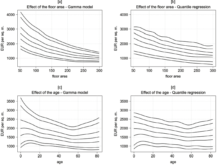
Figure 3 shows the posterior mean effects of the floor area and the age of the building with the other covariates again being held constant at the average effect. In order to facilitate comparability we show the effects of a particular covariate on the same scale for both the Gamma model and the quantile regression. While the quantiles of the floor area have a convex shape in the Gamma model (panel [a]), the effects are more or less linear in the quantile regression, displayed in panel [b]. Furthermore, the variance considerably differs in the Gamma model with a large variance for small houses and vice versa.

Figure 3:

5%-, 10%-, 30%-, 50%-, 70%-, 90%-, 95%-quantiles of selected continuous structural level-1 covariates for the Gamma model (left column) and the quantile regression (right column), evaluated at the average effect.

The results of the age are very similar between the Gamma model (Figure 3, panel [c]) and quantile regression (panel [d]) for the lower quantiles up to the median. For the 5%- and the 10%-quantile the effects seem to be almost linear and slightly decreasing over the whole range of the age (at least for an age exceeding seven years). The 30%- and the 50%-quantiles are linearly decreasing up to an age of 55 years and are almost constant or slightly increasing afterwards. The upper quantiles, in contrast, considerably differ between the two models: In the quantile regression, the effects still decline linearly up to 55 years and reverse hereafter. In the Gamma model the effects more and more tend to a quadratic shape.

Figure 4 shows the estimated quantiles of selected spatial covariates again at the average effect. The 5%- and the 10%-quantiles of the purchase power index (panels [a] and [b]) are almost linearly increasing both for the Gamma model and the quantile regression. For the remaining quantiles we find a tendency towards undulating effects that are more pronounced in the Gamma model. However, the decreasing effect for low and high index points should not be overstated due to only a very small number of municipalities with such purchase power indices.

Figure 4:

5%-, 10%-, 30%-, 50%-, 70%-, 90%-, 95%-quantiles of selected spatial level-2 and level-3 covariates for the Gamma model (left column) and the quantile regression (right column), evaluated at the average effect.

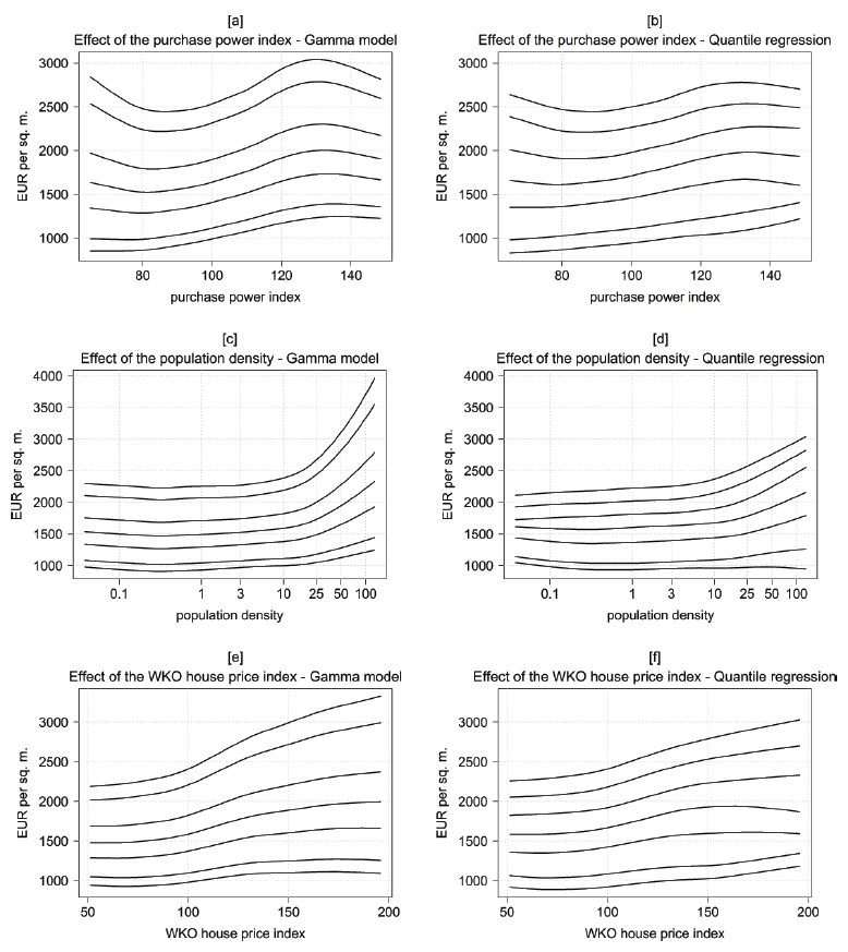
The quantiles of the population density show that over the whole distribution of prices there is almost no effect for sparsely inhabited areas, neither in the Gamma model nor in the quantile regression. In contrast, for densely populated areas there is a slightly positive effect for the lower quantiles and an ever-growing positive effect for the upper quantiles. Especially the effects of the 90%- and the 95%-quantile of highly populated areas are much more pronounced in the Gamma model than in the quantile regression.

The results of the WKO house price index are quite similar in both models with effects that are more or less linearly increasing for all different quantiles. The slope is rather small for the lower quantiles and somewhat higher for the upper quantiles.

The spatial covariates, defined on the municipal- and the district-level, explain spatial heterogeneity to a certain extent, so we call this the explained spatial heterogeneity. The remaining i.i.d. spatial random effects ${ϵ}_5\mathrm{,}{ϵ}_{\mathrm{5,6}}$ and ${ϵ}_{\mathrm{5,6,3}}$ as well as the correlated district specific effect $f_{\mathrm{5,6,2}}^{mrf}(district)$ account for unexplained spatial heterogeneity.

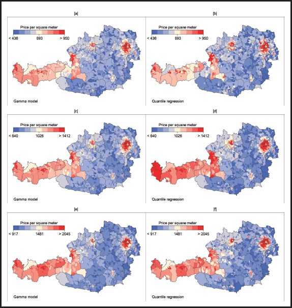
Figure 5 (colored) visualizes the distribution of the total spatial heterogeneity over Austria that is composed by the sum of the explained and the unexplained heterogeneity, evaluated again at the average effect. For the sake of illustration we restrict the analysis to the 10%-, 50%- and 90%-quantiles. We find considerably higher house prices in the western counties of Austria as well as in the city of Linz and the metropolitan area of Vienna. This effect can consistently be observed for all quantiles. Especially for the median, the spatial heterogeneity seems to be more pronounced in the quantile regression compared to the Gamma model.

Figure 5:

Distribution of total spatial heterogeneity in the 10% (top row), 50% (middle row) and 90% (bottom row) quantile over Austria (evaluated at the average effect) for the Gamma model (left column) and the quantile regression (right column).

In order to select a final model and discriminate between quantile and Gamma regression as the best distributional model we calculate mean weighted errors that allow to compare the predictive ability of the models for each individual quantile. The calculation is based on a five-fold cross validation. According to the detailed analysis in Section B of the Supplement, see particularly Table 4, the Gamma model yields better predictions for all quantiles compared to the quantile regression.

4 Conclusion

This article analyses the distribution of house prices using Bayesian structured additive distributional and quantile regression models. Extending the work of Brunauer et al. (2013) we do not restrict our analysis to the conditional mean but additionally concentrate on conditional quantiles of house prices in order to summarize their whole distribution and to estimate uncertainty in real estate valuation. The article is based on two conceptually different approaches: Distributional STAR models, on the one hand, assume a specific parametric probability distribution of the response and model some or all of its parameters in dependence of covariates. Semiparametric quantile regression, in contrast, directly models the different quantiles of the response as a function of covariates without a specific distribution assumption. Model choice is based on proper scoring rules and mean weighted errors. We identify a model based on the Gamma distribution to be most suitable for our data, giving new insights into the distribution of house prices.

One challenge of distributional regression, the selection of variables to enter the regression specification as well as the selection of appropriate modelling strategies (such as linear vs. nonlinear for continuous covariates) has not been considered in this article. Rather, we focus on the comparison of different regression specifications beyond the mean and considered a pre-selection of variables that was guided by earlier analyses of similar data. To overcome this limitation one could combine of our multilevel models with the effect selection priors proposed in Klein et al. (2021).

Our findings are of great practical interest, especially for investors who seek for evaluating the uncertainty of real estate market values. In this context, the large variation in the variance that we have identified over the domain of some covariates is remarkable. As a consequence, our approach is able to provide more reliable estimates of the distribution of the value of real estate portfolios compared to standard models. Of course, these results as well are valuable for financial institutions or supervisors when evaluating collateral and deriving capital requirements.

Our work and, more importantly, our lives have been significantly influenced by Brian D. Marx and we are very grateful to be able to contribute to this special issue devoted to his memory. Brian was not only a source of inspiration when it comes to statistical modelling in general and smoothing effects of continuous covariates in particular, he was a unique character that was able to create an enjoyable and inspiring atmosphere wherever we met him. Spending time with Brian at one of the many International Workshops on Statistical Modelling or when he was teaching short courses in Göttingen and Innsbruck always left us with smiling faces as well as new insights. We will dearly miss you Brian!

Supplementary materials

Supplementary materials for this article are available online.

Supplemental Material for A multilevel analysis of real estate valuation using distributional and quantile regression by Alexander Razen, Wolfgang Brunauer, Nadja Klein, Thomas Kneib, Stefan Lang, Nikolaus Umlauf, in Statistical Modelling