
Abstract
Over the course of the COVID-19 pandemic, Generalized Additive Models (GAMs) have been successfully employed on numerous occasions to obtain vital data-driven insights. In this article we further substantiate the success story of GAMs, demonstrating their flexibility by focusing on three relevant pandemic-related issues. First, we examine the interdepency among infections in different age groups, concentrating on school children. In this context, we derive the setting under which parameter estimates are independent of the (unknown) case-detection ratio, which plays an important role in COVID-19 surveillance data. Second, we model the incidence of hospitalizations, for which data is only available with a temporal delay. We illustrate how correcting for this reporting delay through a nowcasting procedure can be naturally incorporated into the GAM framework as an offset term. Third, we propose a multinomial model for the weekly occupancy of intensive care units (ICU), where we distinguish between the number of COVID-19 patients, other patients and vacant beds. With these three examples, we aim to showcase the practical and ‘off-the-shelf’ applicability of GAMs to gain new insights from real-world data.
Introduction
From the early stages of the COVID-19 crisis, it became clear that looking at the raw data would only provide an incomplete picture of the situation, and that the application of principled statistical knowledge would be necessary to understand the manifold facets of the disease and its implications (Panovska-Griffiths, 2020; Pearce et al., 2020). Statistical modelling has played an important role in providing decision-makers with robust, data-driven insights in this context. In this article, we specifically highlight the versatility and practicality of Generalized Additive Models (GAMs). GAMs constitute a well-known model class, dating back to Hastie and Tibshirani (1987), who extended classical Generalized Linear Models (Nelder and Wedderburn, 1972) to include non-parametric smooth components. This framework allows the practitioner to model arbitrary target variables that follow a distribution from the exponential family to depend on covariates in a flexible manner. Due to the duality between spline smoothing and normal random effects, mixed models with Gaussian random effects are also encompassed in this model class (Kimeldorf and Wahba, 1970). One can justifiably claim that the model class is one of the main work-horses in statistical modelling (see Wood, 2017 and Wood, 2020 for a comprehensive overview of the most recent advances) and numerous authors have already used this model class for COVID-19-related data analyses. As research on topics related to COVID-19 is still developing rapidly, a complete survey of applications is impossible; hence, we here only highlight selected applications, sorted according to the topic they investigate. Many applications analyse the possibly non-linear and delayed effect of meteorological factors (including, e.g., temperature, humidity, and rainfall) on COVID-19 cases and deaths (see Goswami et al., 2020; Prata et al., 2020; Ward et al., 2020; Xie and Zhu, 2020). While the results for cold temperatures are consistent across publications in that the risk of dying of or being infected with COVID-19 increases, the findings for high temperatures diverge between studies from no effects (Xie and Zhu, 2020) to U-shaped effects (Ma et al., 2020). Logistic regression with a smooth temporal effect, on the other hand, was used to identify adequate risk factors for severe COVID-19 cases in a matched case-control study in Scotland (McKeigue et al., 2020). In the field of demographic research, Basellini and Camarda (2021) investigate regional differences in mortality during the first infection wave in Italy through a Poisson GAM with Gaussian random effects that account for regional heterogeneities. With fine-grained district-level data, Fritz and Kauermann (2022) present an analysis confirming that mobility and social connectivity affect the spread of COVID-19 in Germany. Wood (2021) shows that UK data strongly suggest that the decline in infections began before the first full lockdown, implying that the measures preceding the lockdown may have been sufficient to bring the epidemic under control. This list of applications illustrates how GAMs have been successfully employed to obtain data-driven insights into the societal and healthcare-related implications of the crisis.
We contribute to this success story by focusing on three applications to demonstrate the ‘off-the-shelf’ usability of GAMs. First, we investigate how infections of children influence the infection dynamics in other age groups. In this context, we detail in which setting the unknown case-detection ratio does not affect the (multiplicative) parameter estimates of interest. Second, we show how correcting for a reporting delay through a nowcasting procedure akin to that proposed by Lawless (1994) can be naturally incorporated in a GAM as an offset term. Here, the application case focuses on the reporting delay of hospitalizations. Third, we propose a prediction model for the occupancy of Intensive Care Units (ICU) in hospitals with COVID-19 and non-COVID-19 patients. We thereby provide authorities with interpretable, reliable and robust tools to better manage healthcare resources.
The remainder of the article is organized as follows: Section 2 shortly describes the available data on infections, hospitalizations and ICU capacities that we use in the subsequent analyses, which are presented in Sections 3, 4 and 5, respectively. We conclude the article in Section 6.
Data
For our analyses, we use data from official sources, which we describe below. Note that our applications are limited to Germany although all of our analyses could be extended to other countries given data availability. We pursue all subsequent analyses on the spatial level of German federal districts, which we henceforth refer to as ‘districts’. This spatial unit corresponds to NUTS 3, the third and most fine-grained category of the NUTS European standard (Nomenclature of Territorial Units for Statistics). We refer to Annex A for a graphical depiction of the spatial resolution of the data.
In addition, the LGL dataset includes information on the hospitalization status of each patient, which is not included in the RKI data, that is, whether or not a case has been hospitalized and the date of hospitalization, if this had occurred. We determine the date on which a hospitalized case is reported to the health authorities by matching the cases across the downloads available on different dates. This is necessary in order to derive the reporting delay for each hospitalization, which is of interest in Section 4.
Analysing associations between infections from different age groups
A central focus during the COVID-19 pandemic is to identify the main transmission patterns of the infection dynamics and their driving factors. In this context, the role of children in schools for the general incidence poses an important question with many socio-economic and psychological implications to it (see Andrew et al., 2020; Luijten et al., 2021). Since findings from previous influenza epidemics have tended to identify the younger population, children aged between 5 and 17, as the key ‘drivers’ of the disease (Worby et al., 2015), the German government ordered school closures throughout the course of the pandemic between spring 2020 and 2021 to contain the pandemic. However, whether these measures were necessary or effective in the case of COVID-19 is still subject to current research (e.g., Perra, 2021). In particular, several studies investigated the global effect of infections among school children, but a general conclusion could not be drawn (see Flasche and Edmunds, 2021; Hippich et al., 2021; Hoch et al., 2021; Im Kampe et al., 2020). In general, we would like to remark that in many studies the main goal was to arrive at conclusions about the susceptibility, severity, and transmissibility of COVID-19 for children (Gaythorpe et al., 2021). On the other hand, we are here primarily interested in quantifying how the incidences of children are associated with the incidences in other age groups. Therefore, we want to assess whether children are key ‘drivers’ of the pandemic. Our analysis is based on aggregated data on the macro level, as opposed to the data on the individual level, which is needed to answer hypotheses, for example, about the susceptibility of a particular child.
Autoregressive model for incidences
To tackle this problem from a statistical point of view, we propose to analyse the infection data using a time-series approach (Fokianos and Kedem, 2004). Let therefore

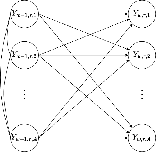
Assumed temporal dependence structure visualized as a directed acyclic graph (DAG)
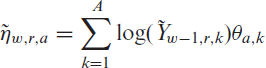
where
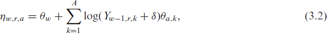
where
Model (3.1) has the important methodological advantage of being able to cope with an unknown case-detection ratio, which is inevitable if there are under-reported cases. This is a key problem in COVID-19 surveillance as not all infections are reported (Li et al., 2020); hence the case-detection ratio (CDR) is typically less than one. Various approaches have been pursued to quantify the number of unreported cases, for example, by estimating the proportion of current infections which are not detected by PCR tests (Schneble et al., 2021a). For demonstration, assume that

infections in the corresponding week
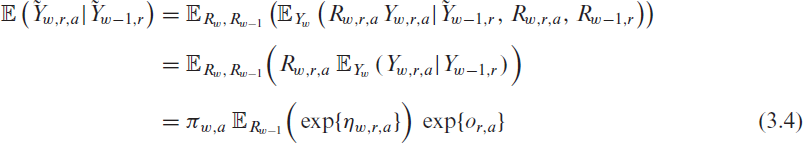
where for clarity we include the random variable as an index in the notation of the expectation. Note that
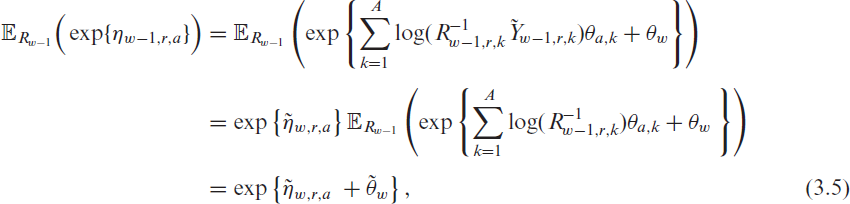
where
and
Hence, combining (3.4) and (3.5) shows that if we fit the model (3.2) to the observed data, which are affected by unreported cases, we obtain the same autoregressive coefficients
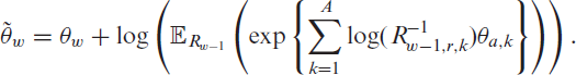
We can now investigate the infection dynamics between different age groups to answer the question brought up at the beginning of Section 3.1. Since the age groups provided by the RKI are too coarse for this purpose, we rely on the data provided by the LGL for Bavaria. For this dataset, we have the age for each recorded case, which, in turn, enables us to define customized age groups. To be specific, we define the age groups of the younger population in line with the proposal of the WHO and UNICEF (2020): 0–4, 5–11, 12–20, 21–39, 40–65, +65. For this analysis, we estimate model (3.1) with data on infections which were registered between 1 and 27 March 2021. The data was downloaded in May 2021; hence reporting delays should have no relevant impact on the analysis. We employ model (3.1) separately for all five analysed age groups to assess how all age groups affect each other. The fitted autoregressive coefficients
Association of previous week’s incidences in different age groups (colour-coded) with the current-week incidences for calendar weeks 9–12 in 2021 stratified by age group (5 age groups correspond to 5 distinct Models)
Association of previous week’s incidences in different age groups (colour-coded) with the current-week incidences for calendar weeks 9–12 in 2021 stratified by age group (5 age groups correspond to 5 distinct Models)
In general, we observe that the autoregressive effects for the own age group, that is,
The results do not come without limitations. First of all, note that the data is observational, not experimental. Hence, we can only draw associative and not causal conclusions from the data without additional assumptions. Moreover, we rely on the given assumptions on the under-reporting. Still, rerunning the analyses for other weeks, shown in the Supplementary Material, yielded similar results, supporting the robustness of our approach and findings. Further, by the beginning of March 2021 around 2.2 million people predominantly from the 65+ age group were already fully vaccinated against COVID-19, which may have an effect on the estimates.
A relevant number of COVID-19 infections lead to hospitalizations, and the incidence of patients hospitalized in relation to COVID-19 is of paramount importance to policymakers for several reasons. First, hospitalized cases are most likely to result in very severe illnesses and deaths, the minimization of which is generally the primary aim of healthcare management efforts. In addition, knowing the number of hospitalized patients is crucial to adequately assess the current state of the healthcare system. Finally, while the number of detected infections depends considerably on testing strategy and capacity, the number of hospitalizations provides a more precise picture of the current situation. For these reasons, hospitalization incidence has been deemed increasingly more relevant by scientists and decisionmakers over the course of the pandemic, and finally became the central indicator for pandemic management in Germany from September 2021, complementing the incidence of reported infections.
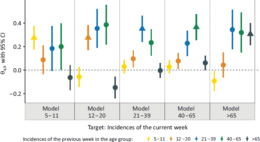
The central problem in calculating the hospitalization incidence with current data is that hospitalizations are often reported with a delay. Such late registrations occur along reporting chains (from local authorities to central registers), but also due to data validity checking at different levels. Visual proof of the degree of this phenomenon is given in Figure 3, which depicts the empirical distribution function of the time (in days) between the date on which a patient is admitted into a Bavarian hospital and the date on which the hospitalization is included in the central Bavarian register. In 2021, only
Cumulative distribution function of the time delay (in days) between hospitalization and its reporting, calculated with data from 1 January to 18 November of 2021, shown separately for the age groups 0–59 and 60+. The curves for both age groups are truncated at a delay of 40 days, when approximately 94.6% of all hospitalizations have been reported
Cumulative distribution function of the time delay (in days) between hospitalization and its reporting, calculated with data from 1 January to 18 November of 2021, shown separately for the age groups 0–59 and 60+. The curves for both age groups are truncated at a delay of 40 days, when approximately 94.6% of all hospitalizations have been reported
Modelling and interpreting current data with only partially observed hospitalization incidences can lead to biased estimates and misleading conclusions, especially if one is interested in the temporal dynamics. To correct for such reporting delays, we utilize ‘nowcasting’ techniques, loosely defined as ‘[t]he problem of predicting the present, the very near future, and the very recent past’ (p. 193, Bańbura et al., 2012). Related methods have been extensively treated in the statistical literature (see, e.g., Höhle and An Der Heiden, 2014; Lawless, 1994) and successfully applied to infections and fatalities data during the current health crisis (De Nicola et al., 2022; Günther et al., 2020; Schneble et al., 2021b). In contrast to these approaches, we here focus on modelling the hospitalization incidences, correcting for delayed reporting through a nowcasting procedure based on the work of Schneble et al. (2021b).
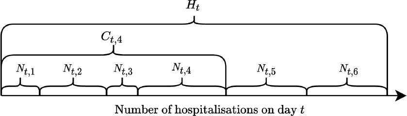
We denote by

To account for the delayed registration of hospitalizations in
In this first step, we estimate the final number of hospitalized patients on day

Illustration of the data setting for
.
indicates hospitalizations reported with a specific delay
, while
denotes all those reported with delay up to
.
denotes the final number of hospitalized cases regardless of the delay with which they were reported, that is with a delay up to the maximum possible,
where

conditional on covariates
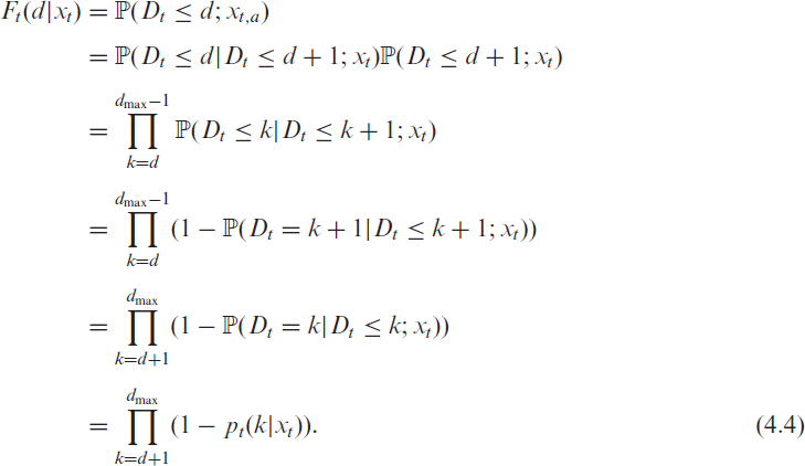
Combining (4.2) and (4.3) allows us to model the delay distribution with incomplete data. We do this separately for two age groups, which we denote by an additional index

with the structural assumption

where
From Figure 4, one can also derive that the proportion of

meaning that the expected number of patients from age group

This equation holds for any delay
In summary, we can fit the logistic regression model given by (4.5) with the available data on hospitalizations. Based on this model, we exploit (4.7) to obtain an estimate for the expected number of hospitalizations from age group
In the second step, we propose a model for the expected value of
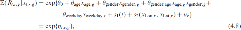
where the linear predictor
Note that, on any given day

where we set

holds. In practice we thereby replace the unknown quantities in the offset with their estimates derived in the previous section. In other words, the delayed reporting is accommodated through an offset in the model using only the reported data

with
As an additional note, we point out that accounting for late registrations works analogously for any model within the endemic–epidemic framework originating in Held et al. (2005). The only difference to the approach presented here is that the exact functional form of the expected value must be adequately accounted for. For instance, if
For the application, we focus on the first two months of the fourth wave of the pandemic in Bavaria, which began towards the end of September 2021. In particular, we consider hospitalizations between 24 September and 18 November, using data reported as of 18 November 2021. We set
Figure 5 maps the raw and corrected rolling weekly sums of hospitalization counts accompanied by the
Comparison of nowcasted (red) and reported (blue) rolling weekly sums of hospitalization counts between 24 September and 18 November 2021, based on data reported as of 19 November 2021. Note: 95% confidence intervals of the nowcast estimates are indicated by the shaded areas. The dashed black lines show the realized weekly sums of hospitalization after 40 days, that is, the maximum delay assumed in our nowcasting model. Results are displayed for the overall population (a) as well as separately for age groups 0–59 (b) and 60+ (c)
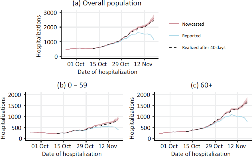
Comparison of nowcasted (red) and reported (blue) rolling weekly sums of hospitalization counts between 24 September and 18 November 2021, based on data reported as of 19 November 2021. Note: 95% confidence intervals of the nowcast estimates are indicated by the shaded areas. The dashed black lines show the realized weekly sums of hospitalization after 40 days, that is, the maximum delay assumed in our nowcasting model. Results are displayed for the overall population (a) as well as separately for age groups 0–59 (b) and 60+ (c)
Turning to the results of the hospitalization model proposed in Section 4.2, the estimated coefficients for all age and gender combinations can be seen in Figure 6. Those estimates reveal considerably lower hospitalization rates for people younger than 35 than all other age groups. We generally observe a positive correlation between age and risk of hospitalization for both genders, that is, older people are more likely to be hospitalized. The only exception to this intuitive finding is seen for men over 80 years, whose expected hospitalization rates are slightly lower than men aged 60 to 79. Statistically significant differences between men and women are visible across all age groups. While women in the youngest and oldest age group tend to have a (slightly) higher hospitalization rate than men, the opposite holds for the other groups.
Estimated linear effects for different age and gender groups in the hospitalization model, where males aged 15–34 are the reference category. Note: Estimated standard deviations are written in brackets
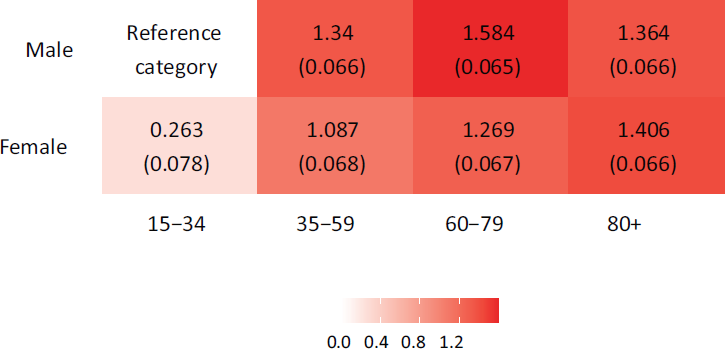
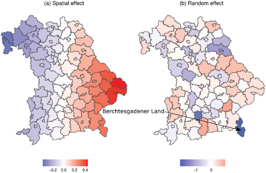
Figure 7 depicts the random and smooth spatial effects (on the log-scale). The smooth effect in Figure 7 (a) paints a clear spatial pattern, with generally higher hospitalization rates in the eastern parts of Bavaria and lower rates in the north-western districts. This structure reflects the pandemic situation in Bavaria during autumn 2021, where we observed the most severe dynamics in those eastern districts. Districts with unexpectedly high or low hospitalization rates (when compared to their neighbouring areas) can be located on the map of the district-specific random intercepts in Figure 7 (b). Contrary to its role as a hotspot during the second wave in autumn 2020, the district with the lowest random effect is Berchtesgadener Land. We estimate an overall variance of
Estimated smooth spatial effect (a) and district-specific random effect (b) in the hospitalization model
The primary aims of healthcare management efforts during a pandemic include minimizing very severe and fatal cases, as well as preventing the overload and collapse of the healthcare system. Information on these very severe cases, among other quantities of interest, can be captured by the ICU occupancy, which is the focus of our third application case.
Multinomial model
We consider the occupancy of ICUs where, as described in Section 2, beds are categorized into the number of vacant beds (

where
One advantage of this multinomial approach is that we implicitly account for displacement effects commonly observed for ICU occupancy data. Over time, as the number of beds occupied by patients infected with COVID-19 rise, both free beds and beds occupied by patients not infected with COVID-19 decrease almost simultaneously. In particular, the ‘displacement’ may be caused by practices such as rescheduling non-urgent operations or other treatments which would have required an ICU stay, which were already common during the first wave of COVID-19 (Stößet al., 2020). These effects lead to negative correlations between the entries in
Taking the number of beds occupied by patients infected with COVID-19 as the reference category, we effectively parametrize pairwise comparisons via

where the linear predictors

where
As stated, the multinomial model has the beneficial property of automatically accounting for displacement effects. Note, however, that patients’ expected length of stay in intensive care may exceed our time unit of one week, as the average stay of COVID-19 patents is about 13 days (see Vekaria et al., 2021). This means that not all beds are completely redistributed at every time point of observation. However, apart from including the previous week’s occupancy in the covariates, our proposed model does not adequately account for this stochastic variability.
We therefore pursue a Bayesian view and let

For the newly allocated beds we still assume a multinomial model:

with
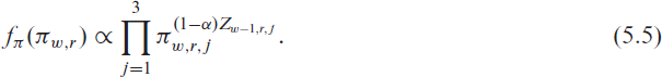
Combining the prior (5.5) with the likelihood from (5.4), leads to the posterior

This, in turn, equals the likelihood resulting from the multinomial model and justifies the use of model (5.2) even though not all beds are allocated weekly. Nevertheless, the central assumption of independent observations in standard uncertainty quantification in GAMs (Wood, 2006) is violated. To correct for this bias, we substitute the canonical covariance of the estimators with the robust sandwich estimator based on M-estimators defined by:

where we set
We now employ the multinomial logistic regression (5.1) to ICU data recorded during the third wave between March and June 2021. For the incidence data used in the covariates, we employ the RKI data; hence we set
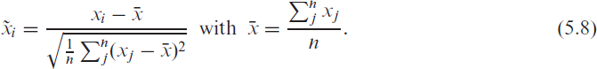
This way, we facilitate the interpretation of associations and guarantee a meaningful comparison between the covariates. Due to space restrictions, we here only present the linear effects from (5.3) and refer to the Supplementary Material for the random and smooth estimates.
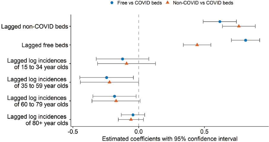
In Figure 8, we visualize the estimated coefficients, including their confidence intervals. The reference category in both pairwise comparisons is COVID-beds; thus, we refer to the two models as free vs COVID beds and non-COVID vs COVID beds. In particular, the coefficients relate to the association between the covariates and the logarithmic odds of a bed not being occupied compared to being occupied by a patient with COVID-19, shown with blue dots in Figure 8. Analogously, the orange triangles in Figure 8 illustrate the estimated association between the covariates and the logarithmic odds of a bed being occupied by a patient not infected with COVID-19 in comparison to a bed being occupied by a patient infected with COVID-19. To demonstrate the uncertainty of each estimate, a 95% confidence interval is added. Keeping the other variables constant, the normalized lagged log-incidences of all age groups generally have a negative effect on the logarithmic odds of both pairwise comparisons. This translates to the finding that an increase in the incidences leads to a decrease in the proportion of non-COVID and free-beds in when compared to COVID beds. The lagged normalized proportion of free and non-COVID beds is estimated to have a stronger, positive association with the logarithmic odds of both pairwise comparisons. We, therefore, expect a higher number of non-COVID beds in the previous week to be followed by a higher number of non-COVID beds in the next week.
Estimated coefficients with confidence interval of the associations between normalized linear covariates included in the multinomial model and the logarithmic odds of a bed being free vs occupied by a patient infected with COVID-19 (blue dots) and the logarithmic odds of a bed being occupied by a patient not infected with COVID-19 vs a patient infected with COVID-19 (orange triangles)
The model can be extended to a forecasting model, as shown in the supplementary material. In particular, we demonstrate how forecasting performance changes over the different waves of the pandemic. In principle, we could also incorporate further covariates like district-specific proportions of vaccinated people. Unfortunately, these numbers are not very reliable and require sophisticated cleaning, so we prefer not to present results in this direction here.
The COVID-19 pandemic poses numerous complex challenges to scientists from different disciplines. Statisticians and epidemiologists, in particular, face the problem of extracting meaningful information from imperfect, incomplete and rapidly changing data. Generalized additive models are a powerful tool that, if used correctly, can help solving some of these challenges. In this work, we have addressed three such challenges where the utilization of GAMs provided meaningful insight.
We investigated whether children are the main drivers of the pandemic under a time-varying case-detection ratio. We modelled hospitalization incidences controlling for delayed registrations, thereby providing both up to dates estimates of current hospitalization numbers as well as insight on the demographic and spatio-temporal drivers of COVID-19. We developed an interpretable predictive tool for ICU bed occupancy that is actively used by the Bavarian government.
We achieved all of those results by using GAMs with different methodological extensions. Nevertheless, the use of our proposed models to extract novel information from the data provided is still subject to both data-related and methodological limitations. In general, our data sources are subject to exogenous shocks (e.g., policy changes) that lead to sudden changes in population behaviour and pose a danger to the validity of our results. Regarding the study of infection dynamics of school kids, revised testing policies hinder the long-range comparability of our findings. In the hospitalization data, the exact date of hospitalization is missing for about 10
We close this work by emphasizing that the nowcasting model can also be used as a stand-alone model. In the German COVID-19 Nowcast Hub (KIT), the described model is used among other nowcasting methods, including the work of Günther et al. (2020) and van de Kassteele et al. (2019), to estimate hospitalization counts on the national and federal state level in Germany. Apart from a systematic evaluation of the different approaches, one of the main goals of this project is to combine individual nowcasts to an ensemble nowcast, which may lead to more accurate estimates.
Appendix: A Spatial unit
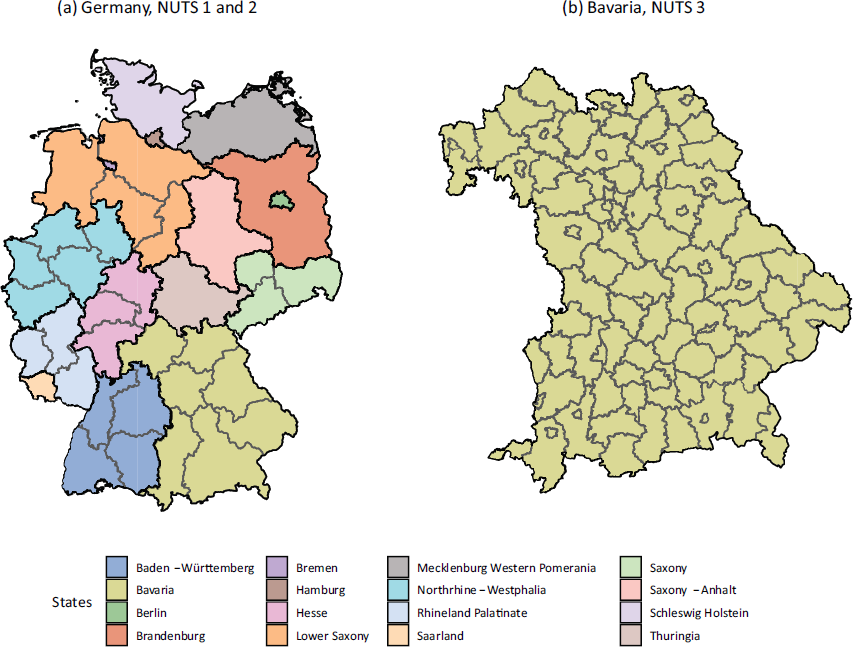
We carried out most modelling endeavours presented in this article on the NUTS 3 level, which is shown on the right side of Figure A.1. The only exception is the Nowcasting model from Section 4.1, where we aggregate all data onto the NUTS 1 level in Bavaria. Moreover, NUTS 1 regions, depicted on the left side of Figure A.1, are the federal states in Germany and Bavaria is one of them. In Section 3 and 4, we are only analysing data from Bavaria, while we employ data from complete Germany in Section 5.
(a): Map of Germany, where the NUTS 1 regions are indicated by the black borders and the different colours. The NUTS 2 regions, on the other hand, are drawn in grey. Note that all NUTS 1 region borders are also NUTS 2 region borders. (b): Map of Bavaria where also the NUTS 3 regions are marked. In the legend, we state the names of each NUTS 1 region
Supplementary materials
Supplementary materials for this article are available online, including additional information on the three application cases. The replication code is available in the following repository: https://github.com/corneliusfritz/Statistical-modelling-of-COVID-19-data .
Supplemental Material for Statistical modelling of COVID-19 data: Putting generalized additive models to work by Cornelius Fritz, Giacomo De Nicola, Martje Rave, Maximilian Weigert, Yeganeh Khazaei, Ursula Berger, Helmut Küchenhoff and Göran Kauermann, in Statistical Modelling
Footnotes
Acknowledgements
We would like to thank Manfred Wildner and Katharina Katz on behalf of the staff of the IfSG Reporting Office of the Bavarian Health and Food Safety Authority (LGL) for cooperatively providing the data used for Sections 3 and 4 and for fruitful discussions on the analysis of the COVID-19 pandemic. We would also like to thank all COVID-19 Data Analysis Group (CODAG) members at LMU Munich for countless beneficial conversations and Constanze Schmaling for proofreading. Moreover, we would like to thank the two anonymous reviewers whose valuable and constructive comments were highly appreciated and led to an improvement of the manuscript.
Declaration of conflicting interests
The authors declared no potential conflicts of interest with respect to the research, authorship and/or publication of this article.
Funding
The work has been partially supported by the German Federal Ministry of Education and Research (BMBF) under Grant No. 01IS18036A. We also acknowledge support of the Deutsche Forschungsgemeinschaft (KA 1188/13-1) and the Bavarian Health and Food Safety Authority (LGL).