Soft-clipping INGARCH models for time series of bounded counts

Abstract

The soft-clipping binomial INGARCH (scBINGARCH) models are proposed as time series models for bounded counts, which have a nearly linear structure and also allow for negative autocor-relations. Conditions that guarantee the existence and certain mixing properties of the scBINGARCH process are derived, and further stochastic properties are discussed. The consistency and asymptotic nor-mality of maximum likelihood estimators are established, and finite-sample properties are studied with simulations. The practical relevance of the scBINGARCH model’s ability to allow for negative parameter and ACF values is demonstrated by some real-data examples.

1 Introduction

Count time series have attracted a lot of interest in research and practice during the last decades, see Weiß (2018) for a survey. These quantitative time series have a range consisting of either the full set of non-negative integers, ${\mathbb{N}}_0=\{\mathrm{0,1,}\dots \}$ (unbounded counts), or a finite subset thereof, $\{\mathrm{0,}\dots \mathrm{,}n\}$ with some $n\in \mathbb{N}=\{\mathrm{1,2,}\dots \}$ (bounded counts). Many count time series models are inspired by the traditional autoregressive moving-average (ARMA) models for real-valued time series, that is, they are defined such that the upcoming observation depends linearly (in some sense) on past observations and possibly further information. This might be achieved by defining ARMA-like recursions using so-called ‘thinning operations’, or by utilizing a regression approach to ensure a linear conditional mean. The latter models are often referred to as the integer-valued generalized autoregressive conditional heteroskedasticity (INGARCH) models, although they are, in fact, closely related to the ARMA models, also see the discussion on p. 74 in Weiß (2018). The cutting feature of such linear count time series models is an ARMA-like autocorrelation structure, that is, their autocorrelation function (ACF) satisfies a set of Yule–Walker equations. As a consequence, moment properties are easily expressed by closed-form formulae. But unlike the original ARMA models, it is problematic (if not even impossible) to allow for negative ACF values, which, in turn, is caused by parameter constraints that are necessary to ensure the non-negative outcomes (counts) for the data-generating process. More precisely, for unbounded counts, an exactly linear model with negative AR parameters is not possible as past observations might be arbitrarily large such that we would end up with a negative conditional mean, which is not allowed for a count random variable (r. v.). For bounded counts with their additional reflecting barrier at $n$ , by contrast, negative ACF values can be achieved but only under rather restrictive conditions. Examples are the binomial AR $(1)$ (BinAR $(1)$ ) model (McKenzie, 1985) and the binomial INARCH $(1)$ (BINARCH $(1)$ ) model (Weiß & Pollett, 2014; Ristić et al., 2016), which are discussed in more detail later in Section 3. If one does not insist on conditional linearity, then one can certainly get rid of such restrictions on parameter and ACF values. An example is given by the binomial logit-ARCH model (Chen et al., 2020), which uses a logit link to ensure the boundedness of the range; also see Chen et al. (2022) for a more general discussion. But then, parameter values are more difficult to interpret, and closed formulae for the ACF and further moments are not available. Further recent articles on bounded INGARCH models are Liu et al. (2022a, 2022b).

To resolve the ‘linearity versus negative ACF’ dilemma for the case of unbounded counts, Weiß et al. (2022) recently proposed the so-called ‘softplus INGARCH model’ to enable both a nearly linear structure and negative ACF (approximately satisfying the Yule–Walker equations), which is achieved by using the softplus link for model definition (see Section 2 for further details). However, the softplus approach cannot be applied to bounded counts as the softplus function is not bounded from above. Therefore, in this article, we develop a novel model family for time series of bounded counts, referred to as the soft-clipping INGARCH models, which are nearly linear and allow for negative ACF values at the same time. In Section 2, we motivate our approach and derive its relation to the soft-clipping function as well as to a type of mollified uniform distribution (also see Appendix A). The soft-clipping function has been discussed previously in the context of neural network activation functions (Klimek & Perelstein, 2020). In particular, we derive conditions that guarantee the existence and certain mixing properties of the soft-clipping binomial INGARCH process (scBINGARCH). Then, we focus on important special cases. In Section 3, the scBINARCH $(1)$ model, which constitutes a rather well-behaved finite Markov chain allowing for likelihood inference, is compared to its exactly linear competitors, the aforementioned BinAR $(1)$ and BINARCH $(1)$ models, which assume an exactly linear relationship between $X_{t-1}$ and $E[X_t|X_{t-1}]$ . Afterwards in Section 4, we show how to extend our findings to the higher-order Markovian scBINARCH $(p)$ models, which allow to model a wide range of autocorrelation structures. In Section 5, in turn, we consider the scBINGARCH $(\mathrm{1,1})$ model, which includes a feedback term and, thus, allows to capture some kind of ‘long memory’. The practical relevance of the scBINGARCH’s ability to allow for negative parameter and ACF values is demonstrated in Section 6 with some real-data examples. Finally, Section 7 concludes and outlines issues for future research.

2 The Soft-clipping approach for bounded counts

2.1 Motivation

To motivate our proposed solution for time series consisting of bounded counts, let us start with a look at INGARCH-type models for processes $(X_t)$ of unbounded counts. Their basic idea is to define the conditional mean at time $t$ , $M_t=E[X_t|{\mathcal{F}}_{t-1}]$ with ${\mathcal{F}}_{t-1}$ being the $\sigma$ -field generated by $\{(X_{t-1}\mathrm{,}{M}_{t-1})\mathrm{,}(X_{t-2}\mathrm{,}{M}_{t-2})\mathrm{,}\dots \}$ , by the recursive scheme

$$M_t=f(a_0+{\displaystyle \sum _{i=1}^p}{a}_i{X}_{t-i}+{\displaystyle \sum _{j=1}^q}{b}_j{M}_{t-j})\mathrm{.}$$

(2.1)

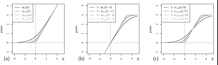
Then, the upcoming count value $X_t$ is generated according to some count distribution having the mean $M_t$ , for example, the Poisson distribution $Poi(M_t)$ . Choosing the response function $f$ as the identity leads to the ordinary and exactly linear INGARCH $(p\mathrm{,}q)$ model of Ferland et al. (2006), but then, the constraints $a_0>0$ and $a_1\mathrm{,}\dots \mathrm{,}{a}_p\mathrm{,}{b}_1\mathrm{,}\dots \mathrm{,}{b}_q\ge 0$ are required to ensure that $M_t>0$ . An intuitive way to overcome these parameter constraints is to choose $f$ in a way that it ensures the correct range of $M_t$ for any parameter values. One might choose $f(x)=\exp (x)$ (log-linear model), but this leads to a distinctly non-linear structure. Another idea would be to choose $f$ as the rectified linear unit function, $ReLU(x)=\max \left\{\mathrm{0,}x\right\}$ , but then $M_t=0$ might happen, which leads to a degenerate count distribution. Therefore, Weiß et al. (2022) proposed to define $f$ as the softplus function $s{p}_c(x)=c\ln (1+\exp (x/c))$ with adjustment parameter $c>0$ (see Mei & Eisner, 2017), which approaches $ReLU(x)$ for $c\to 0$ , also see Figure 1(a).

Figure 1

Plots of different (a) softplus functions $s_c(x)$ , (b) reversed softplus functions $n-s_c(n-x)$ with $n=3$ and (c) rescaled soft clipping functions $ns{c}_{\frac{c}{n}}(\frac{x}{n})$ with $n=3$

Let us now turn to the case of bounded counts $(X_t)$ with upper limit $n\in \mathbb{N}$ . INGARCH-type models for bounded counts (Weiß & Pollett, 2014; Ristić et al., 2016; Chen et al., 2020) can be defined by the recursive scheme

$$M_t=f(n{\alpha }_0+{\displaystyle \sum _{i=1}^p}{\alpha }_i{X}_{t-i}+{\displaystyle \sum _{j=1}^q}{\beta }_j{M}_{t-j})\mathrm{.}$$

(2.2)

Because of the bounded range, one may also use the following equivalent characterization based on the normalized conditional mean, $P_t=\frac{1}{n}{M}_t$ , together with $f^{*}(x)=\frac{1}{n}f(n\cdot x)$ :

$$P_t=f^{*}({\alpha }_0+{\displaystyle \sum _{i=1}^p}{\alpha }_i{X}_{t-i}/n+{\displaystyle \sum _{j=1}^q}{\beta }_j{P}_{t-j})\mathrm{.}$$

(2.3)

Then, the counts $X_t|{\mathcal{F}}_{t-1}$ are emitted by, for example, the conditional binomial distribution $Bin(n\mathrm{,}{P}_t)$ ; further options for the conditional distribution of $X_t|{\mathcal{F}}_{t-1}$ are briefly discussed in Section 7. Using the identity as the response function $f$ (Weiß & Pollett, 2014; Ristić et al., 2016) requires strict parameter constraints, whereas the choice of the inverse logit function (Chen et al., 2020) leads to a distinctly non-linear model. It is also clear that neither $ReLU(x)$ nor $s{p}_c(x)$ could control an additional upper bound $n\in \mathbb{N}$ , whereas the function $n-s{p}_c(n-x)$ , which approaches $\min \left\{n\mathrm{,}x\right\}$ for $c\to 0$ (also see Figure 1(b)), would be unbounded from below. Defining $f$ as the clipped ReLU function $cReL{U}_n(x)=\min \left\{n\mathrm{,}\max \right\{\mathrm{0,}x\left\}\right\}$ (Cai et al., 2017) causes the problem of a possibly degenerate count distribution with all probability mass in either $0$ or $n$ , also recall the above discussion of $ReLU(x)$ . Furthermore, $cReL{U}_n(x)$ is not continuously differentiable in $0$ and $n$ . Thus, the idea is to combine $s{p}_c(x)$ and $n-s{p}_c(n-x)$ in such a way that we end up with a smoothed type of $cReL{U}_n(x)$ . Here, it is crucial to note the decomposition $cReL{U}_n(x)=\max \left\{\mathrm{0,}x\right\}-x+\min \left\{n\mathrm{,}x\right\}$ , which is easily verified. Inspired by this, we choose the response function $f(x)$ in (2.2) as

$$s{p}_c(x)-x+n-s{p}_c(n-x)=n-x+c\ln (\frac{1+\exp (\frac{x}{c})}{1+\exp (\frac{n-x}{c})})=c\ln (\frac{1+\exp (\frac{x}{c})}{1+\exp (\frac{x-n}{c})})\mathrm{.}$$

f equals a re-scaled type of the soft clipping function (Klimek & Perelstein, 2020), that is, of

$$s{c}_c(x)=c\ln \left(\frac{1+\exp (\frac{x}{c})}{1+\exp (\frac{x-1}{c})}\right)\mathrm{,}$$

namely $f(x)=ns{c}_{c/n}(x/n)$ as plotted in Figure 1(c). Properties of the soft clipping function (A.1) are discussed in Appendix A, where we also show the relation to a type of mollified uniform distribution (in analogy to the relation between the logit link and the logistic distribution). To sum up, we refer to $(X_t)$ following (2.2) as a soft-clipping INGARCH model if the response function $f$ is equal to

$$f(x)=ns{c}_{\frac{c}{n}}(\frac{x}{n})=c\ln (\frac{1+\exp (\frac{x}{c})}{1+\exp (\frac{x-n}{c})})\mathrm{.}$$

(2.4)

Equivalently, the soft-clipping INGARCH model can be defined based on the normalized conditional mean in (2.3), by using

$$f^{*}(x)=s{c}_{c^{*}}(x)=c^{*}\ln \left(\frac{1+\exp (\frac{x}{c^{*}})}{1+\exp (\frac{x-1}{c^{*}})}\right)\text{\hspace{1em}\hspace{1em}with}{c}^{*}=\frac{c}{n}\mathrm{.}$$

(2.5)

For a numerically more stable implementation of (2.4) and (2.5), we use (A.4).

Adapting the properties of $s{c}_c(x)$ in Appendix A, we know that $f(x)$ in (2.4) takes values in $(\mathrm{0,}n)$ , it approaches $cReL{U}_n(x)$ for $c\to 0$ , also see Figure 1(c), and it is differentiable in $x$ up to any order. The maximal deviation of (2.4) to $cReL{U}_n(x)$ is in $x=0$ and $x=n$ (of opposite sign), and it is of absolute size $c\ln (2/(1+\exp (-\frac{n}{c})))$ . Analogous results hold for the normalized version of $f$ , that is, for $f^{*}:ℝ\to (\mathrm{0,1})$ in (2.5), which approaches $cReLU$ for $c\to 0$ , with maximal deviation to $cReLU(x)$ in $x=0$ and $x=1$ .

2.2 The soft-clipping binomial INGARCH model

Let $(X_t)$ with range $\{\mathrm{0,}\dots \mathrm{,}n\}$ be defined by (2.3) and (2.5). If the counts $X_t|P_t$ are emitted by the binomial distribution $Bin(n\mathrm{,}{P}_t)$ , then we abbreviate the model as ‘soft-clipping BINGARCH’ (scBINGARCH), with ‘B’ like binomial. So, the scBINGARCH $(p\mathrm{,}q)$ model is defined by

$$X_t|{\mathcal{F}}_{t-1}\sim Bin(n\mathrm{,}{P}_t)\text{\hspace{1em}with}{P}_t=s{c}_c({\alpha }_0+{\displaystyle \sum _{i=1}^p}{\alpha }_i{X}_{t-i}/n+{\displaystyle \sum _{j=1}^q}{\beta }_j{P}_{t-j})\mathrm{.}$$

(2.6)

While the model would be well-defined also without further restrictions, we assume that $\left|{\alpha }_i\right|\mathrm{,}\left|{\beta }_j\right|<1$ for $i=\mathrm{1,}\dots \mathrm{,}p$ and $j=\mathrm{1,}\dots \mathrm{,}q$ to prevent a degenerate behaviour. In (2.6), for the sake of readability, we simply write $c$ instead of $c^{*}$ for the adjustment parameter. While ${\alpha }_1\mathrm{,}\dots \mathrm{,}{\beta }_q$ play the role of dependence parameters, ${\alpha }_0$ can be understood as the (normalized-)mean parameter, see the discussion in the last paragraph of Section 2.2. Thus, to ensure the interpretability of ${\alpha }_0$ , a further constraint such as ${\alpha }_0\in (\mathrm{0,1}+p+q)$ appears to be reasonable. Note that $s{c}_c(1-x)=1-s{c}_c(x)$ because of the point symmetry in $(\frac{1}{2}\mathrm{,}\frac{1}{2})$ (Appendix A), so the ‘mirrored version’ of model (2.6), that is, where $Y_t=n-X_t$ and $Q_t=1-P_t$ , satisfies $Y_t\sim Bin(n\mathrm{,}{Q}_t)$ with the same dependence parameters as in (2.6) and a modified intercept term.

Lemma 1. With the aforementioned parameter constraints, and with $c>0$ , it follows that there exist ${ϵ}_1\mathrm{,}{ϵ}_2>0$ such that

$$P_t\in [{ϵ}_1\mathrm{,1}-{ϵ}_2]\text{\hspace{1em}\hspace{1em}forall}t\mathrm{.}$$

We have $0\le X_t/n\le 1$ , and for a cReLU-INGARCH model, it would also be possible that $P_t$ reaches the bounds $0$ and $1$ of this range. However, Lemma 2.2 states that for a scBINGARCH model with positive $c$ , the conditional normalized mean $P_t$ is truly bounded away from $0$ to $1$ . The proof of Lemma 2.2 is simple: considering the extreme parameter scenarios ${\alpha }_1\mathrm{,}\dots \mathrm{,}{\beta }_q\in \{-\mathrm{1,1}\}$ and the extreme cases $X_s/n\mathrm{,}{P}_s\in \left\{\mathrm{0,1}\right\}$ for $s<t$ , and using that $s{c}_c(x)$ is strictly monotone increasing in $x$ , it follows that $P_t>s{c}_c(-p-q)>0$ and $P_t<s{c}_c(1+2p+2q)<1$ . Note that these bounds are only established to obtain theoretical results, but they do not imply any relevant restrictions for practice. For example, for $c=0.01$ and $p+q=1$ , we have the lower bound $s{c}_{0.01}(-1)\approx 3.7\cdot {10}^{-46}$ , and for $c=0.1$ still $s{c}_{0.1}(-1)\approx 4.5\cdot {10}^{-6}$ , which is a negligible deviation from zero.

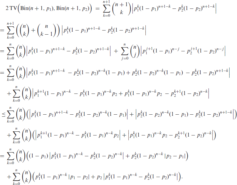
As another preliminary step towards proving the existence of the scBINGARCH process defined by (2.6), we present the following auxiliary result about the total variation (TV) distance between two binomial distributions.

Lemma 2. Let $n\in \mathbb{N}$ and $p_1\ge p_2\ge n/\delta >0$ for some $\delta >0$ . Then,

$$TV(Bin(n\mathrm{,}{p}_1)\mathrm{,}Bin(n\mathrm{,}{p}_2))\le 1-{(1-|p_1-p_2|)}^n\le 1-{(\frac{p_2}{p_1})}^n\le 1-\exp (-\delta |p_1-p_2|)\mathrm{.}$$

The proof of Lemma 2 is provided in Appendix B.1. Note that $n/\delta$ just denotes a truly positive lower bound for $p_2$ . For (2.6), the existence of such a lower bound is ensured by Lemma 1.

Now we proceed in analogy to Weiß et al. (2022) and derive a theorem stating the existence and uniqueness of a stationary distribution of (2.6), as well as its absolute regularity (see Bradley, 2005 for a survey on strong-mixing concepts), provided that some regularity conditions are satisfied. For this purpose, we show that conditions (A1)–(A3) in Doukhan & Neumann (2019) hold such that their Corollary 2.1 as well as Theorems 2.1 and 2.2 are applicable. Our results are summarized in Theorem 1 as follows.

Theorem 1. If the scBINGARCH $(p\mathrm{,}q)$ process (2.6) satisfies ${\displaystyle {\sum }_{j=1}^q}\left|{\beta }_j\right|<1$ and ${\displaystyle {\sum }_{i=1}^p}\max \left\{\mathrm{0,}{\alpha }_i\right\}+{\displaystyle {\sum }_{j=1}^q}\max \left\{\mathrm{0,}{\beta }_j\right\}<1$ , then the following assertions hold:

The Markov process $(Z{}_t)$ defined by $Z{}_t=(X_t\mathrm{,}\dots \mathrm{,}{X}_{t-p+1}\mathrm{,}{P}_t\mathrm{,}\dots \mathrm{,}{P}_{t-q+1})$ possesses a unique stationary distribution;

A stationary version of $(X_t)$ is absolutely regular with $\beta$ -mixing coefficients bounded by $C{\gamma }^{\sqrt{k}}$ for some constant $C>0$ , some $\gamma \in (\mathrm{0,1})$ , and time lag $k\in \mathbb{N}$ ;

A stationary version of $(X_t\mathrm{,}{P}_t)$ is ergodic.

The proof of Theorem 1 is provided in Appendix B.2. As in Weiß et al. (2022), let us point out that ${\displaystyle {\sum }_{i=1}^p}\left|{\alpha }_i\right|+{\displaystyle {\sum }_{j=1}^q}\left|{\beta }_j\right|<1$ would be a sufficient (but not necessary) condition for Theorem 1 to hold.

Before discussing important special cases of the scBINGARCH family in more detail, let us present some further general results. By definition (2.6), the conditional mean and variance are given by $E[X_t|{\mathcal{F}}_{t-1}]=n{P}_t$ and $V[X_t|{\mathcal{F}}_{t-1}]=n{P}_t(1-P_t)$ , respectively. Here, it is interesting to compare with the ordinary BINGARCH model, which uses a linear link. Let $P_t^{*}$ denote the normalized mean of such a truly linear model, that is, $P_t=f^{*}(P_t^{*})$ . Then, it holds that $V[X_t|{\mathcal{F}}_{t-1}]>n{P}_t^{*}(1-P_t^{*})$ , that is, the conditional variance of the scBINGARCH model is larger than if using a linear link. This can be seen by considering that $x(1-x)$ is maximized at 0.5, and that the soft-clipping function is mapping each value towards 0.5: because of the curvature of $s{c}_c(x)$ , we have $|s{c}_c(x)-0.5|<|x-0.5|$ .

There is no explicit formula for the unconditional mean $E[X_t]$ , but our computations show that it is generally close to the value obtained by plugging in the parameters into the formula for the unconditional mean of the exactly linear BINGARCH model, that is, $E[X_t]\approx n{\alpha }_0/(1-{\displaystyle {\sum }_{i=1}^p}{\alpha }_i-{\displaystyle {\sum }_{j=1}^q}{\beta }_j)$ (RistiÀ et al. 2016, Theorem 8). This approximation can also be justified as follows. By Taylor’s formula, we have $E[X_t]=nE[s{c}_c(P_t^{*})]=n{\displaystyle {\sum }_{k=0}^{\infty }}s{c}_c^{(k)}(0.5)/k!\cdot E[(P_t^{*}-{0.5)}^k]$ . Note that $s{c}_c\text{'}(0.5)=\tanh (1/(4c))\approx 1$ for small $c$ , while $s{c}_c(0.5)=0.5$ and $s{c}_c{\text{'}}^{\prime }(0.5)=0$ . Thus, a second-order Taylor approximation yields $E[X_t]\approx nE[s{c}_c(0.5)+s{c}_c\text{'}(0.5)(P_t^{*}-0.5)+0]\approx nE[P_t^{*}]$ , as in a truly linear model. Analogously, the Yule–Walker equations in Theorem 9 and Example 2 of RistiÀ et al. (2016) are used to approximate the autocorrelation properties of the scBINGARCH process, irrespective of any parameter constraints.

3 The soft-clipping BINARCH(1) model

As the first important special case of the scBINGARCH family (2.6), we discuss the scBINARCH $(1)$ model (that is, $p=1$ and $q=0$ ), the model recursion of which can be summarized as

$$X_t|{\mathcal{F}}_{t-1}\sim Bin(n\mathrm{,}{P}_t)\text{\hspace{1em}with}{P}_t=s{c}_c({\alpha }_0+{\alpha }_1{X}_{t-1}/n)\mathrm{.}$$

(3.1)

Since $P_t\in (\mathrm{0,1})$ is guaranteed if $c>0$ (also recall Lemma 1), the transition probabilities of this finite Markov chain are always truly positive, that is, it is primitive and thus ergodic with a unique stationary solution. In addition, it is also $\varphi$ -mixing with geometrically decreasing weights (Weiß, 2018), which strengthens Theorem 1. Obviously, ${\alpha }_1=0$ leads to independent and identically distributed (i. i. d.) binomial counts, so we have a true Markov model only if ${\alpha }_1\cancel{=}0$ . But otherwise, no parameter restrictions are required. Note that the above conclusions would also hold if taking the beta-binomial (zero-inflated binomial) distribution for emitting the counts, that is, with an additional dispersion (zero) parameter, because this distribution has a truly positive probability mass function on whole $\{\mathrm{0,}\dots \mathrm{,}n\}$ as well.

3.1 Model properties

We shall now compare the properties of this nearly linear model with two well-established exactly linear finite Markov chains: the ordinary BINARCH $(1)$ model (Weiß & Pollett, 2014) defined by using the identity link instead of the soft-clipping one,

$$X_t|{\mathcal{F}}_{t-1}\sim Bin(n\mathrm{,}{a}_0+a_1{X}_{t-1}/n)\text{\hspace{1em}withconstraints}{a}_0\mathrm{,}{a}_0+a_1\in (\mathrm{0,1})\mathrm{,}$$

(3.2)

and the BinAR $(1)$ model by McKenzie (1985). The latter uses the binomial thinning operation ‘ $\circ$ ’ (Steutel & van Harn, 1979) for model definition, given by $\alpha \circ X|X\sim Bin(X\mathrm{,}\alpha )$ for $\alpha \in (\mathrm{0,1})$ . Let $\pi \in (\mathrm{0,1})$ and $\rho \in (\max \{\frac{-\pi }{1-\pi }\mathrm{,}\frac{1-\pi }{-\pi }\}\mathrm{,}1)$ , denote $\beta :=\pi (1-\rho )$ and $\alpha :=\beta +\rho$ . Then, the BinAR $(1)$ model is defined by

$$X_t=\alpha \circ X_{t-1}+\beta \circ (n-X_{t-1})\mathrm{.}$$

(3.3)

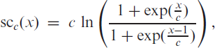
Setting $\rho =a_1$ and $\pi =a_0/(1-a_1)$ , the BinAR $(1)$ and BINARCH $(1)$ model have the same mean and ACF, namely $E[X_t]=n\pi$ and $ACF(k)={\rho }^k$ at lag $k$ , and also their parameter constraints agree (thus, they have a common grey region in Figure 2). But they differ in their variance: while the BinAR $(1)$ model has the binomial variance $V[X_t]=n\pi (1-\pi )$ , the BINARCH $(1)$ model exhibits extra-binomial variation, namely $V[X_t]=n\pi (1-\pi )/(1-(1-\frac{1}{n}){\rho }^2)$ , see Weiß & Pollett (2014). Equivalently, the binomial index of dispersion (BID), defined as $nV[X_t]/(E[X_t](n-E[X_t]))$ , equals 1 for the BinAR $(1)$ model, and $1/(1-(1-\frac{1}{n}){\rho }^2)$ for the BINARCH $(1)$ model. Note that $ACF(k)$ might be negative at odd lags, because $\rho$ might be negative. However, the maximal extend of negativity depends on the actual normalized mean, $\frac{1}{n}E[X_t]=\pi$ , see the grey regions in Figure 2. The black regions in Figure 2 are the corresponding moment properties of the scBINARCH $(1)$ model, which have been computed numerically exactly by utilizing the scBINARCH $(1)$ model’s Markov property: solving the invariance equation corresponding to scBINARCH $(1)$ ’s transition matrix, we get the stationary marginal distribution and, thus, arbitrary lag- $k$ distributions, from which we compute the discrete moments by simple summation. The black region consists of dots computed for a grid of parameter values for $({\alpha }_0\mathrm{,}{\alpha }_1)$ .

Figure 2

Plots of attainable pairs of $ACF(1)$ against $\frac{1}{n}E[X_t]$ for different upper bounds $n$ , where black region corresponds to scBINARCH $(1)$ model with $c=0.01$ , and grey region to BinAR $(1)$ model (or equivalently, BINARCH $(1)$ model)

Before looking at the scBINARCH $(1)$ model’s potential for negative $ACF(1)$ values, a more general discussion is necessary. In contrast to, for example, the Gaussian AR $(1)$ model, where $ACF(1)$ can attain any value within $(-\mathrm{1,1})$ independent of the actual mean, the possibility for negative $ACF(1)$ values is usually limited for discrete-valued processes (also see Lin et al., 2014, Section 2). For $n=1$ , all three models agree with a (re-parametrized) general binary Markov chain, that is, the grey region in Figure 2 cannot be exceeded in that case (for negative ACF values of more general binary time series, also see Jentsch & Reichmann (2019)). For $n>1$ , the BinAR $(1)$ and BINARCH $(1)$ model are still not able to exceed this grey region, whereas the scBINARCH $(1)$ model reaches more and more pairs $(\frac{1}{n}E[X_t]\mathrm{,}ACF(1))$ with increasing $n$ , see the black regions in Figure 2. So this model is much more flexible with respect to negative ACF values.

The next question to be analyzed is the ‘extent of linearity’ that is achieved by the scBINARCH $(1)$ model. For this purpose, for diverse model parameterizations, we computed the values of the normalized mean, the BID, and the partial ACF (PACF) at lags 1–3. These are compared with the corresponding ‘linear values’, that is, the values obtained by plugging in the parameters into the above formulae of the BINARCH $(1)$ model (irrespective of any parameter constraints). Note that the latter model has PACF values equal to 0 for lags $k\ge 2$ . The obtained results are summarized in the tables of Supplement S.1, where we have to compare the ‘sc’ values to the ‘lin’ values. It can be seen that the linearity improves if the normalized mean approaches 0.5, which is reasonable in view of the areas plotted in Figure 2. It is also plausible that the linearity improves with increasing $n$ . But the most important factor is certainly given by the parameter $c$ , recall Figure 1(c), where the values printed for $c=0$ were computed by using the response function $cReLU(x)$ instead of $s{c}_c(x)$ . This boundary case is not relevant for applications in practice because of the problems explained in Section 2, but it serves as the ‘best case’ regarding the attainable linearity. Comparing $c>0$ with $c=0$ , it can be seen that there are sometimes notable deviations from linearity for $c=\mathrm{0.1,0.05}$ , whereas $c=0.025$ and especially $c=0.01$ often lead to nearly identical values as $c=0$ . So for practice, $c\le 0.025$ appears to be a reasonable choice to obtain a nearly linear model. Nevertheless, there are a few scenarios where we observe deviations from linearity even for $c=0$ , namely low $\pi$ (especially $\pi =0.1$ ) and low $n$ in the case of strongly negative dependence parameters. This can be explained from our discussion in Figure 2, where we realized that Markov chains cannot reach ACF values being arbitrarily close to $-1$ in such scenarios. But except for these extreme cases, the scBINARCH $(1)$ model with low $c$ (such as $c=0.01$ ) does very well in imitating linearity.

3.2 Likelihood-based statistical inference

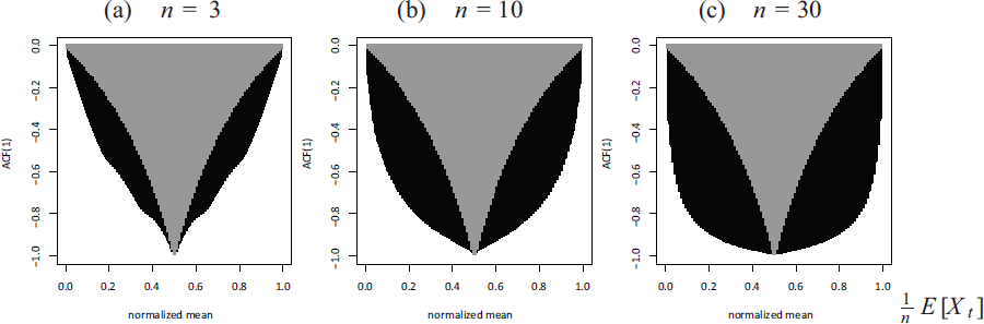
Results regarding likelihood-based inference, especially about the asymptotics of the conditional maximum likelihood (CML) estimator of the scBINARCH $(1)$ ’s model parameter vector $\theta =({\alpha }_0\mathrm{,}{\alpha }_1)$ , follow immediately once Condition 5.1 of Billingsley (1961) has been shown. Let us focus on parameter estimation from a given time series $x_1\mathrm{,}\dots \mathrm{,}{x}_T$ of length $T\in \mathbb{N}$ here. The scBINARCH $(1)$ ’s conditional log-likelihood function is given by

$$\begin{array}{l}\mathcal{l}(\theta )=\ln L(\theta ;x_1)={\displaystyle \sum _{t=2}^T}\ln p_{x_t|x_{t-1}}\mathrm{,}\text{\hspace{1em}where}\hfill \\ p_{j|i}=\left(\begin{array}{c}n\\ j\end{array}\right)s{c}_c{({\alpha }_0+{\alpha }_1\frac{i}{n})}^j{(1-s{c}_c({\alpha }_0+{\alpha }_1\frac{i}{n}))}^{n-j}\hfill \end{array}$$

(3.4)

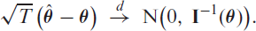
denotes the transition probabilities $p_{j|i}=P(X_t=j|X_{t-1}=i)$ of this finite Markov chain (which are truly positive for $c>0$ ). The CML estimate $\theta$ of $\theta$ is obtained by numerically maximizing $\mathcal{l}(\theta )$ , where approximate moment estimates (obtained by applying the approximate moment relations of Section 3.1 to the respective sample moments) might be used as initial values. If $c>0$ , the existence of a consistent CML estimator, $\theta \to \theta$ almost surely, is ensured, which is also asymptotically normally distributed according to

$$\sqrt{T}(\theta -\theta )\stackrel{d}{\to }N(\mathrm{0,}I{}^{-1}(\theta ))\mathrm{,}$$

(3.5)

where $I{}^{-1}(\cdot )$ denotes the expected Fisher information. (3.5) follows from Theorems 2.1 and 2.2 of Billingsley (1961), and $I(\theta )$ is non-singular according to Billingsley (1961, p. 24. The proof of this assertion is provided in Appendix B.3.

Simulations results (with 10 000 replications per scenario and with $c=0.01$ ) for checking the finite-sample performance of $\theta$ are summarized in Supplement S.2. It can be seen that the CML estimation performs rather well even for such small sample sizes as $T=50$ . We have a low bias, quickly decreasing standard errors (s. e.), and the approximate s. e. obtained from the Hessian of $\mathcal{l}$ agree quite well with the simulated s. e. in the mean.

Remark 1. Note that our main intention is to use the scBINGARCH models as approximations of truly linear models. Thus, we specify the adjustment parameter $c>0$ in advance, chosen sufficiently small such that approximate linearity holds (such as $c=0.01$ as recommended in Section 3.1). If one wants to use a scBINGARCH model as a truly non-linear model, with $c\gg 0$ , then it would be relevant to include $c$ into estimation. This issue is briefly discussed at the end of Appendix 2.3. Our simulation experiments showed that a reasonable finite-sample performance is only achieved if $c$ is sufficiently distant from 0. This is plausible as we recognized in Section 3.1 that models with $c\le 0.025$ are hard to distinguish in their stochastic properties.

4 Higher-order soft-clipping BINARCH models

According to (2.6), the scBINARCH $(1)$ model discussed in previously in Section 3 is extended to a $p$ th-order Markov model with $p>1$ by the recursive scheme

$$X_t|{\mathcal{F}}_{t-1}\sim Bin(n\mathrm{,}{P}_t)\text{\hspace{1em}with}{P}_t=s{c}_c({\alpha }_0+{\displaystyle \sum _{i=1}^p}{\alpha }_i{X}_{t-i}/n)\mathrm{.}$$

(4.1)

Model (4.1) constitutes a counterpart to the truly linear BINARCH $(p)$ model of RistiÀ et al. (2016) but with much weaker parameter constraints. In particular, the moment properties in Theorems 1–2 of RistiÀ et al. (2016) hold true in approximation, even if negative parameter values are employed. As in Section 3, results exceeding those of Theorem 1 are derived by utilizing the Markov properties of the scBINARCH $(p)$ model. The idea is to consider the process of vectors $X{}_t=(X_t\mathrm{,}\dots \mathrm{,}{X}_{t-p+1}{)}^{\top }$ , which again constitutes a finite Markov chain. Given $c>0$ , the corresponding 1-step-ahead transition probabilities $p_{j|i}=P(X{}_t=j|X{}_{t-1}=i)$ are non-zero iff $j_2=i_1$ , ..., $j_p=i_{p-1}$ , namely

$$p_{j|i}={\delta }_{j_2\mathrm{,}{i}_1}\cdots {\delta }_{j_p\mathrm{,}{i}_{p-1}}\cdot \left(\begin{array}{c}n\\ j_1\end{array}\right)P_i^{j_1}{(1-P_i)}^{n-j_1}\text{\hspace{1em}with}{P}_i=s{c}_c({\alpha }_0+{\displaystyle \sum _{k=1}^p}{\alpha }_k\frac{i_k}{n})\mathrm{.}$$

(4.2)

Furthermore, the $p$ -step-ahead transition probabilities are truly positive throughout. Thus, we can conclude on the existence of a unique stationary solution (ergodic and $\varphi$ -mixing) as well as on likelihood inference like in Section 3, also see the analogous arguments in RistiÀ et al. (2016).

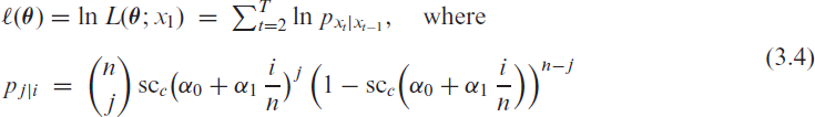
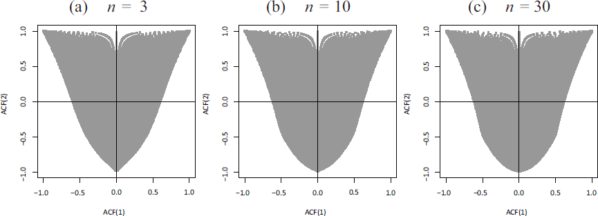
To get an idea about the abilities of the scBINARCH model for explaining different autocorrelation structures, we created some ACF $(2)$ –ACF $(1)$ plots for the scBINARCH $(2)$ model in Figure 3, in analogy to Figures 6(b) and 7 of Jentsch & Reichmann (2019). More precisely, for the values $n\in \left\{\mathrm{3,10,30}\right\}$ , ${\alpha }_1\mathrm{,}{\alpha }_2\in \{-\mathrm{0.99,}-\mathrm{0.98,}\dots \mathrm{,0.99}\}$ , ${\alpha }_0=0.5(1-{\alpha }_1-{\alpha }_2)$ , and $c=0.01$ , we computed the values of $ACF(1)\mathrm{,}ACF(2)$ and plotted them against each other. Note that the ordinary BINARCH $(2)$ model of RistiÀ et al. (2016) only allows for non-negative values of the AR parameters, that is, it only allows to achieve pairs $(ACF(1)\mathrm{,}ACF(2))$ in the top-right quadrants of Figure 3. So it becomes clear that the novel scBINARCH $(2)$ model is much more flexible w. r. t. the achievable autocorrelation structures, with increasing range of ACF pairs for increasing $n$ in analogy to Figure 2.

Figure 3

Plots of attainable pairs of $ACF(2)$ against $ACF(1)$ for the scBINARCH $(2)$ model, for different upper bounds $n$ and with $c=0.01$

5 Including a feedback term: scBINGARCH(1,1) model

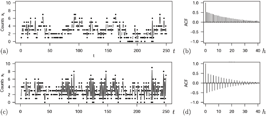
Within families of INGARCH-type models, the model order $(p\mathrm{,}q)=(\mathrm{1,1})$ is a rather common choice in practice, as it constitutes a parsimonious way of providing some kind of ‘long memory’ (in the sense of a very slowly decreasing ACF like in Figure 4), see Fokianos (2011). This is achieved by including the feedback term $M_{t-1}$ (or $P_{t-1}$ , respectively) into the model recursion (2.6) for $X_t|{\mathcal{F}}_{t-1}$ ,

$$X_t|{\mathcal{F}}_{t-1}\sim Bin(n\mathrm{,}{P}_t)\text{\hspace{1em}with}{P}_t=s{c}_c({\alpha }_0+{\alpha }_1{X}_{t-1}/n+{\beta }_1{P}_{t-1})\mathrm{.}$$

(5.1)

Figure 4

Plots of a sample path and ACF $(h)$ of a scBINGARCH $(\mathrm{1,1})$ process with $n=10$ , $c=0.01$ , ${\alpha }_0=0.3(1-{\alpha }_1-{\beta }_1)$ , and (a–b) ${\alpha }_1=0.25$ , ${\beta }_1=0.70$ ; (c–d) ${\alpha }_1=-0.25$ , ${\beta }_1=-0.70$

The model order $(\mathrm{1,1})$ considered in (2.14) is also a special case of the beta-binomial GARCH $(\mathrm{1,1})$ model in Chen et al. (2022), as the scBINGARCH $(\mathrm{1,1})$ process satisfies their contraction condition (2.4), see our derivations for (A2) in Appendix B.2. (4.1) results in a dependence of $X_t$ on all past observations $X_{t-h}$ , but with (approximately) exponentially decreasing weight for increasing $h$ , see the discussions in Section 3 of Fokianos (2011) or Example 4.1.4 of Weiß (2018). For the illustrative examples shown in Figure 4, a sample path of length ${10}^4$ was simulated (the time series plot refers to the first $T=250$ observations) and used to compute the sample ACF. Since $|{\alpha }_1+{\beta }_1|=0.95$ is close to $1$ in both cases, the ACF converges only slowly towards $0$ .

The existence of a unique stationary solution (ergodic and $\beta$ -mixing) is ensured by Theorem 1. But it could also be concluded from Propositions 1 and 2 in Davis & Liu (2016), as the conditional binomial distribution belongs to the one-parameter exponential family (and since the soft-clipping function satisfies a contraction condition, recall the proof of Theorem 1 in Appendix B.2). Theorems 1 and 2 in Davis & Liu (2016), in turn, are now used to conclude in the following result about CML estimation.

Theorem 1. If the scBINGARCH $(\mathrm{1,1})$ process (5.1) satisfies the conditions of Theorem 1, then the CML estimator $\theta \to \theta$ almost surely, and it is asymptotically normally distributed,

$$\sqrt{T}(\theta -\theta )\stackrel{d}{\to }N(\mathrm{0,}I{}^{-1}(\theta ))\mathrm{.}$$

The proof of Theorem 1 is provided in Appendix B.4. Note that Theorems 1 and 2 in Cui & Zheng (2017) provide an extension of Davis & Liu (2016) to general model orders $(p\mathrm{,}q)$ . For the model order $(\mathrm{1,1})$ considered in Theorem 1, in turn, also the results in Chen et al. (2022) could have been used for a proof.

The finite-sample performance of $\theta$ was again investigated by simulations (with 10 000 replications per scenario and with $c=0.01$ ), see Supplement S.2. This time, however, in analogy to the findings of Weiß al. (2022), we recognize that clearly larger sample sizes are required for achieving a good estimation performance, say $T\ge 250$ . Then, the performance is better if $|{\alpha }_1+{\beta }_1|$ is much smaller than 1. For the simulation scenarios with $|{\alpha }_1+{\beta }_1|=0.70$ , we have a notable bias even for $T=250$ , especially for ${\beta }_1$ . This is plausible as ${\beta }_1$ controls the length of the process memory. It is also interesting to note that the bias for ${\beta }_1$ often increases with increasing $n$ , while we usually have a stable bias for ${\alpha }_1$ . Simulated and approximate s. e., by contrast, agree quite well in the mean.

6 Data examples

6.1 Geyser eruption data

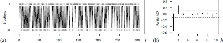
As our first data example, we consider the geyser eruption data analyzed by Jentsch & Reichmann (2019). This binary time series (so $n=1$ ) of length $T=299$ refers to successive eruptions of the Old Faithful Geyser (Data provided in R’s MASS package, https://cran.r-project.org/package=MASS), where the value 1 (0) was recorded if the eruption duration was at least (less than) three minutes. The geyser eruption data exhibit strong negative autocorrelations with significant sample PACF values for lags $\le 2$ , see Figure 5. Therefore, Jentsch & Reichmann (2019) fitted the second-order autoregressive gbAR $(2)$ model from their generalized binary ARMA (gbARMA) family to these data and showed the adequacy of this model fit. Jentsch & Reichmann (2019) developed their gbARMA family as an extension of the so-called NDARMA model by Jacobs & Lewis (1983): By adding a switching facility to the NDARMA’s multinomial selection mechanism, they circumvented the NDARMA’s disadvantage of only capturing positive ACF values. In what follows, we demonstrate that our novel scBINARCH $(p)$ model may serve as a ‘more user-friendly’ alternative to the gbAR model $(p)$ , while the scBINGARCH $(p\mathrm{,}q)$ model leads to a different ACF than the gbARMA $(p\mathrm{,}q)$ model for $q>1$ (‘long memory’ vs traditional ARMA ACF).

Figure 5

Time series plot and sample PACF of geyser eruption data

Computing CML estimates for the AR parameters ${\alpha }^{(1)}\mathrm{,}{\alpha }^{(2)}$ and the error term’s mean ${\mu }_e$ of the gbAR $(2)$ model, we get ${\widehat{\alpha }}^{(1)}\approx -0.393$ , ${\widehat{\alpha }}^{(2)}\approx 0.270$ , and ${\widehat{\mu }}_e\approx 1.000$ , where ${\widehat{\mu }}_e$ actually equals the upper bound used for the box constraints of ${\mu }_e\in (\mathrm{0,1})$ . The corresponding value of Akaike’s information criterion (AIC) computes as $\approx 259.8$ . Note that Jentsch & Reichmann (2019) used the AIC for model order selection, with the result $p=2$ nicely confirming the outcome of the sample PACF in Figure 5. The conditional distribution of our scBINARCH $(p)$ model (4.1) from Section 4 and, thus, numerical likelihood computations appear to be slightly more easy to implement than for the gbAR $(p)$ model. Furthermore, the parameterization with the intercept parameter ${\alpha }_0$ instead of the error term’s mean ${\mu }_e$ turns out to be advantageous, as we do not get in conflict with the box constraints. Fitting the model orders $p=\mathrm{1,2,3}$ and using $c=0.01$ , we get the estimates $({\widehat{\alpha }}_0\mathrm{,}{\widehat{\alpha }}_1)\approx (\mathrm{1.106,}-0.647)$ with $AIC\approx 272.5$ , $({\widehat{\alpha }}_0\mathrm{,}{\widehat{\alpha }}_1\mathrm{,}{\widehat{\alpha }}_2)\approx (\mathrm{0.867,}-\mathrm{0.530,0.270})$ with $AIC\approx 259.8$ , and $({\widehat{\alpha }}_0\mathrm{,}{\widehat{\alpha }}_1\mathrm{,}{\widehat{\alpha }}_2\mathrm{,}{\widehat{\alpha }}_3)\approx (\mathrm{0.884,}-\mathrm{0.511,0.256,}-0.036)$ with $AIC\approx 262.6$ , respectively. Thus, we confirm the choice of the model order $p=2$ . The identical AIC values (up to the given numerical precision) for the gbAR $(2)$ and scBINARCH $(2)$ models follow from nearly identical stochastic properties of both model fits.

Within the scBINGARCH family, also the scBINGARCH $(\mathrm{1,1})$ model (4.1) from Section 5 is a plausible candidate model, as the sample ACF values $-\mathrm{0.538,0.478,}-\mathrm{0.346,0.318,}-\mathrm{0.256,}\dots$ for lags $h=\mathrm{1,2,}\dots$ are slowly decaying in absolute extent. CML estimation leads to $({\widehat{\alpha }}_0\mathrm{,}{\widehat{\alpha }}_1\mathrm{,}{\widehat{\beta }}_1)\approx (\mathrm{1.530,}-\mathrm{0.674,}-0.516)$ with $AIC\approx 259.5$ . While the tiny advantage in terms of AIC should not be overestimated for practical purposes, it is interesting to note that the fitted scBINGARCH $(\mathrm{1,1})$ model has ACF values $-\mathrm{0.540,0.478,}-\mathrm{0.379,0.307,}-\mathrm{0.246,}\dots$ being more close to those of the sample ACF than the ACF values $-\mathrm{0.551,0.496,}-\mathrm{0.359,0.272,}-\mathrm{0.203,}\dots$ of the fitted scBINARCH $(2)$ model. Thus, in summary, the scBINARCH model can be used as an alternative to the gbAR model, as it leads to nearly identical stochastic properties except a reparameterization, while the full scBINGARCH model has the ability to describe a slowly decaying ACF.

6.2 Air quality data

As our second application, let us consider the air quality data (Data provided as online supplementary material for Liu et al., 2022a.) discussed by Liu et al. (2022a, 2022b). For 30 Chinese cities, they analyzed a time series of daily air quality levels (December 2013–July 2019, so length $T=2068$ ). Here, air quality is measured on an ordinal scale with levels $s_0=\text{`excellen}{\text{t}}^{\prime }$ to $s_5=\text{`severelypollute}{\text{d}}^{\prime }$ . But for modeling purposes, Liu et al. (2022a) used a ‘rank-count approach’ as in Weiß (2020), that is, the ordinal r. v. $Y_{t\mathrm{,}i}$ at time $t$ in city $i$ is substituted by $s_{X_{t\mathrm{,}i}}$ with $X_{t\mathrm{,}i}$ being a bounded-counts r. v. with $n=5$ . Then, they applied a linear INGARCH $(\mathrm{1,1})$ model to these data, where the conditional distribution is a truncated Poisson distribution with additional zero and one inflation. This ‘ZOB Poisson’ distribution was used by Liu et al. (2022a) as the categories $s_0$ and $s_1$ turned out to be dominant in the data (‘normalcy-dominant’ categorical data). Certainly, the conditional binomial distribution of our scBINGARCH $(\mathrm{1,1})$ model is not able to explain zero and one inflation, so we do not propose it as an alternative model for the full set of time series. But for some of the time series, our scBINGARCH $(\mathrm{1,1})$ model performs well even without the zero-one-inflation feature. Thus, our subsequent discussion shall focus on two such exemplary series. For future research, it is recommended to develop a zero-one-inflated scBINGARCH (scZOBINGARCH) model for dealing with the whole set of air quality time series.

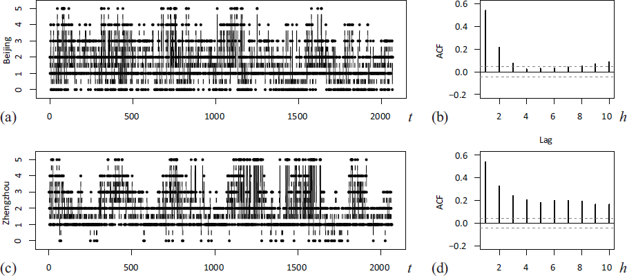
We consider the count time series $(x_{t\mathrm{,}i})$ corresponding to Beijing ( $i=1$ ) and Zhengzhou ( $i=2$ ) as examples. Plots of these time series as well as their sample ACFs are provided in Figure 6. For the Zhengzhou series $(x_{t\mathrm{,2}})$ in (b), we have a slowly decaying ACF as to be expected for INGARCH $(\mathrm{1,1})$ -type data. For the Beijing series $(x_{t\mathrm{,1}})$ in (a), by contrast, the ACF decays rather quickly such that the model choice INGARCH $(\mathrm{1,1})$ is not clear in advance. But following Liu et al. (2022a), we fit an scBINGARCH $(\mathrm{1,1})$ model (with $c=0.01$ ) to both time series.

Figure 6

Time series plot and sample ACF of air quality data for (a–b) Beijing and (c–d) Zhengzhou

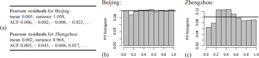
For the Beijing series $(x_{t\mathrm{,1}})$ , we get the CML estimates $({\widehat{\alpha }}_0\mathrm{,}{\widehat{\alpha }}_1\mathrm{,}{\widehat{\beta }}_1)\approx (\mathrm{0.180,0.595,}-0.161)$ , that is, a negative estimate for the feedback parameter ${\beta }_1$ . Such a negative value is not possible for ZOB-INGARCH $(\mathrm{1,1})$ model of Liu et al. (2022a), as all parameters are restricted to non-negative values. Accordingly, the estimate ‘0.0000’ is reported in Table 3 of Liu et al. (2022a). Thus, it is interesting to compare the ACFs of the fitted models to the sample ACF in Figure 6(b), where the fitted models’ ACF was computed as the sample ACF of a simulated sample path of length ${10}^4$ . We get the ACF values $\mathrm{0.546,0.232,0.096,0.036}$ for our scBINGARCH $(\mathrm{1,1})$ fit and $\mathrm{0.519,0.270,0.144,0.075}$ for the ZOB-INGARCH $(\mathrm{1,1})$ fit reported by Liu et al. (2022a)], while the sample ACF takes the values $\mathrm{0.539,0.214,0.073,0.022}$ for lags 1–4. So we recognize a better agreement for our scBINGARCH $(\mathrm{1,1})$ model, that is, the possibility for negative parameter values is clearly advantageous. Also the ACF values of the scBINGARCH $(\mathrm{1,1})$ ’s standardized Pearson residuals in Figure 7(a) are not significant on a 5%-level, confirming that the serial dependence structure is captured adequately. Furthermore, the model’s conditional distribution for $X_t|X_{t-1}\mathrm{,}\dots$ appears adequate, as the residuals’ mean is close to 0, the variance is only slightly larger than 1, and the PIT histogram in Figure 7(b) is close to uniformity; see Weiß (2018, Section 2.4) for details on these diagnostic tools. While the conditional properties of the data are very well described by the fitted scBINGARCH $(\mathrm{1,1})$ model, it is not fully able to mimic the marginal distribution: we have a close agreement between the means, 0.317 versus 0.321 (model vs data) but the BIDs 1.297 versus 1.410 are a bit more distant. More flexibility w. r. t. zero and one inflation could help to better explain the marginal dispersion.

Figure 7

Model diagnostics for scBINGARCH $(\mathrm{1,1})$ fits: sample statistics of Pearson residuals in (a), and PIT histogram for (b) Beijing and (c) Zhengzhou

For the Zhengzhou series $(x_{t\mathrm{,2}})$ , by contrast, all CML estimates are positive, namely $({\widehat{\alpha }}_0\mathrm{,}{\widehat{\alpha }}_1\mathrm{,}{\widehat{\beta }}_1)\approx (\mathrm{0.146,0.494,0.136})$ . We do not only have a close agreement between the model’s and data’s ACF, namely $\mathrm{0.536,0.324,0.236,}\dots$ versus $\mathrm{0.534,0.336,0.207,}\dots$ , also the non-significant values of the Pearson residuals’ ACF in Figure 7(a) confirm the adequacy of the modelled dependence structure. Regarding the marginal distribution, we now have an even closer agreement between the means (0.391 vs 0.396) and BIDs (1.287 vs 1.260) than for the Beijing series. The reason might be given by the fact that only few zeros are observed in Figure 6(c), that is, we do not have inflation in both zero and one. This time, however, there are some reservations with respect to the conditional distributions of $X_t|X_{t-1}\mathrm{,}\dots$ : while mean and variance of the Pearson residuals in Figure 7(a) are close to their target values 0 and 1, respectively, the PIT histogram exhibits an asymmetric behaviour. So mean and variance of the conditional distribution are adequately described by the scBINGARCH $(\mathrm{1,1})$ fit but not its shape. To sum up, the scBINGARCH model is able to flexibly adapt to diverse types of dependence structure, because it is not subject to unduly stringent parameter restrictions. It is not the perfect choice for the air quality data, as it is not able to explain the zero and one inflation. The air quality data also seem to exhibit some yearly pattern, so the inclusion of covariates into the scBINGARCH model might be helpful in this regard. Thus, such extensions appear to be an interesting direction for future research.

7 Conclusions

The scBINGARCH family for time series of bounded counts was proposed as an extension of the linear BINGARCH model, as it gets by with less severe parameter restrictions. In particular, it behaves like the linear BINGARCH model for positive parameter values, but it also allows for negative parameter and thus ACF values. This was achieved by using the nearly linear soft-clipping function as the response function. It was shown that the moment properties of the scBINGARCH model are generally well approximated by simply using the moment formulae from the exactly linear model; this approximation is less accurate only for extreme parameter scenarios. We established the existence and mixing properties for the scBINGARCH model, as well as the consistency and asymptotic normality of the CML estimator. The finite sample performance of the CML estimator was studied by simulations, and the practical relevance of the scBINGARCH model was demonstrated with real-data examples.

However, the data examples also made clear that further research is needed for the model. In particular, the conditional binomial distribution seems to be too restrictive for some applications. Future research could therefore turn to the development of, for example, a beta-binomial scINGARCH model (that is, with an additional parameter for controlling the extend of extra-binomial variation), also see Chen et al. (2022), or to a zero-inflated (or even zero-one-inflated) scINGARCH model (that is, with additional parameter(s) for controlling the zero (and one) probability), with the latter being motivated by the air quality data discussed in Section 6.2. Also, recall Section 3 regarding the Markov case. The air quality example also gives rise to think of a spatio-temporal extension, as there might be some spatial dependence between the air quality of the 30 cities.

Appendices

Appendix A Soft clipping and mollified uniform distribution

The (unit) clipped ReLU function is defined by clipping the identity function to the interval $[\mathrm{0,1}]$ , that is, by $cReLU(x)=\min \left\{\mathrm{1,}\max \right\{\mathrm{0,}x\left\}\right\}$ Cai et al. (2017). A smoothed version of it, the soft clipping function, was proposed by Klimek & Perelstein (2020) as

$$s{c}_c(x)=c\ln \left(\frac{\exp (\frac{x}{c})+1}{\exp (\frac{x-1}{c})+1}\right)=\frac{1}{2}+c\ln \text{}(\cosh (\frac{x}{2c}))-c\ln \text{}(\cosh (\frac{x-1}{2c}))\mathrm{,}c>0.$$

(A.1)

Let us derive important properties of the soft clipping function. It satisfies

$$s{c}_c(x)\in (\mathrm{0,1})\mathrm{,}\underset{x\to -\infty }{{\displaystyle \lim }}s{c}_c(x)=\mathrm{0,}\underset{x\to +\infty }{{\displaystyle \lim }}s{c}_c(x)=\mathrm{1,}$$

and it is point symmetric in $(\frac{1}{2}\mathrm{,}\frac{1}{2})$ . $s{c}_c(x)$ approaches the clipped ReLU function for $c\to 0$ . It is infinitely differentiable, with the first derivative being given by

$$s{c}_{c^{\prime }}(x)=\underset{\in (\mathrm{0,1})}{\underset{ุ}{\frac{\exp (\frac{x}{c})}{\exp (\frac{x}{c})+1}}}\underset{\in (\mathrm{0,1})}{\underset{ุ}{\frac{1-\exp (-\frac{1}{c})}{1+\exp (\frac{x-1}{c})}}}=\frac{\sinh (\frac{1}{2c})}{2\cosh (\frac{x}{2c})\cosh (\frac{x-1}{2c})}\in (\mathrm{0,1})\mathrm{.}$$

(A.2)

Thus, $s{c}_c(x)$ is strictly monotone increasing from 0 to 1, but its increase is weaker than that of $cReLU(x)$ on $(\mathrm{0,1})$ . Therefore, the maximal deviation between $s{c}_c(x)$ and $cReLU(x)$ is in $x=\mathrm{0,1}$ , given by $\pm s{c}_c(0)$ . Note that $s{c}_{c^{\prime }}(x)$ approaches the unit rectangular function $1_{[\mathrm{0,1}]}(x)$ for $c\to 0$ , where the indicator function $1_A(x)$ equals 1 (2.0) if $x\in A$ ( $x\cancel{\in }A$ ). Finally, the soft clipping function is related to the softplus function by

$$s{c}_c(x)=s{p}_c(x)-x+1-s{p}_c(1-x)\mathrm{,}$$

(A.3)

in analogy to the decomposition $cReLU(x)=\max \left\{\mathrm{0,}x\right\}-x+\min \left\{\mathrm{1,}x\right\}$ . Inserting the equality $s{p}_c(x)=\max \left\{\mathrm{0,}x\right\}+c\ln (1+\exp (-\left|\frac{x}{c}\right|))$ Wiemann et al. (2021) into (A.3), we can rewrite the soft clipping function as

$$s{c}_c(x)=cReLU(x)+c\ln \text{}(1+\exp (-\left|\frac{x}{c}\right|))-c\ln \text{}(1+\exp (-\left|\frac{1-x}{c}\right|))\mathrm{,}$$

(A.4)

which, together with the log1p function, allows for a numerically stable implementation of $s{c}_c(x)$ .

Figure A1

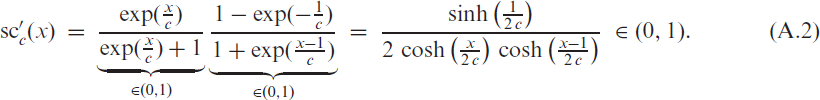
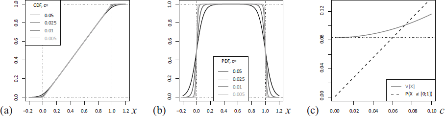
Soft/mollified uniform distribution with scale parameter $c$ . Plots of (a) CDF and (b) PDF for different $c$ against $x$ . (c) Plots of variance and ‘out of unit interval’-probability against $c$

Besides serving as a response function in regression modeling, the soft clipping function is also related to the uniform distribution. Note that $cReLU(x)$ just equals the cumulative distribution function (CDF) of the (unit) uniform distribution, $U(\mathrm{0,1})$ , see Chapter 26 in Johnson et al. (1995). Since $s{c}_c(x)$ from (A.1) is itself a CDF, see Figure A1 (a) for some plots, the corresponding distribution might be thought of as a ‘soft uniform distribution’, which has the full set of real numbers, $ℝ$ , as its range but which approaches $U(\mathrm{0,1})$ for $c\to 0$ . Its probability density function (PDF) is then given by (A.2), see Figure A1 (b) for illustration. Its quantile function $s{c}_c^{-1}:(\mathrm{0,1})\to ℝ$ equals

$$s{c}_c^{-1}(y)=c\ln (\frac{\exp (\frac{y}{c})-1}{1-\exp (\frac{y-1}{c})})=y+c\ln \text{}(1-\exp (-\frac{y}{c}))-c\ln \text{}(1-\exp (-\frac{1-y}{c}))\mathrm{,}$$

(A.5)

where the latter version can again be implemented using the log1p function. It is easily seen that this distribution is equal to the convolution of $U(\mathrm{0,1})$ with the logistic distribution $L(\mathrm{0,}c)$ having mean 0 and scale parameter $c$ , see Chapter 23 in Johnson et al. (1995). Therefore, the ‘soft uniform distribution’ might also be referred to as a ‘mollified uniform distribution’ in the sense of Friedrichs (1944), using a logistic mollifier. The decomposition $X=U+L$ with independent summands $U\sim U(\mathrm{0,1})$ and $L\sim L(\mathrm{0,}c)$ can be utilized for moment calculations. For example, the mean and variance of the soft/mollified uniform distribution are given by $E[X]=\frac{1}{2}$ and $V[X]=\frac{1}{12}+c^2{\pi }^2/3$ , respectively. Figure A1(c) plots the variance $V[X]$ against $c$ (which converges to $1/12$ for $c\to 0$ ) as well as the probability of falling outside the unit interval, that is, $P(X\cancel{\in }[\mathrm{0,1}])=2\cdot s{c}_c(0)\approx 2\ln (2)\cdot c$ .

Appendix B Derivations

B.1 Proof of Lemma 2

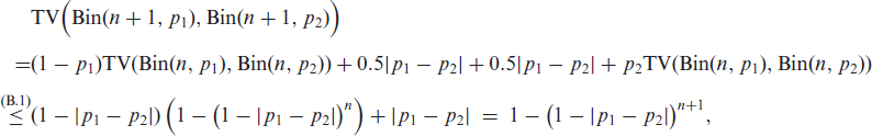
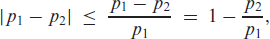
For the discrete binomial distribution, the TV distance is computed as (Gibbs & Su, 2002, p. 424)

$$TV(Bin(n\mathrm{,}{p}_1)\mathrm{,}Bin(n\mathrm{,}{p}_2))=0.5{\displaystyle \sum _{k=0}^n}\left(\begin{array}{c}n\\ k\end{array}\right)|p_1^k{(1-p_1)}^{n-k}-p_2^k{(1-p_2)}^{n-k}|\mathrm{.}$$

The proof of the first inequality in Lemma 2,

$$TV(Bin(n\mathrm{,}{p}_1)\mathrm{,}Bin(n\mathrm{,}{p}_2))\le 1-{(1-|p_1-p_2|)}^n\mathrm{,}$$

(B.1)

is done by induction. Recall that $p_1\ge p_2$ such that $|p_1-p_2|=p_1-p_2$ . For the initial case $n=1$ , we get

$$TV(Bin(\mathrm{1,}{p}_1)\mathrm{,}Bin(\mathrm{1,}{p}_2))=|p_1-p_2|=1-(1-|p_1-p_2|)$$

such that (B.1) holds. So let us turn to the inductive step. Given that the proposed inequality (B.1) holds for some $n\in \mathbb{N}$ , we have for $n+1$ that

$$\begin{array}{l}\begin{array}{l}2\text{TV}(\text{Bin}(n+1,p_1),\text{Bin}(n+1,p_2))={\displaystyle \sum }_{k=0}^{n+1}\left(\begin{array}{c}n+1\\ k\end{array}\right)\left|p_1^k{(1-p_1)}^{n+1-k}-p_2^k{(1-p_2)}^{n+1-k}\right|\hfill \end{array}\\ \begin{array}{l}={\displaystyle \sum }_{k=0}^{n+1}\left(\left(\begin{array}{c}n\\ k\end{array}\right)+\left(\begin{array}{c}n\\ k-1\end{array}\right)\right)\left|p_1^k{(1-p_1)}^{n+1-k}-p_2^k{(1-p_2)}^{n+1-k}\right|\hfill \end{array}\\ \begin{array}{l}={\displaystyle \sum }_{k=0}^n\left(\begin{array}{c}n\\ k\end{array}\right)\left|p_1^k{(1-p_1)}^{n+1-k}-p_2^k{(1-p_2)}^{n-k}(1-p_1)+p_2^k{(1-p_2)}^{n-k}(1-p_1)-p_2^k{(1-p_2)}^{n+1-k}\right|\hfill \end{array}\\ \begin{array}{l}={\displaystyle \sum }_{k=0}^n\left(\begin{array}{c}n\\ k\end{array}\right)\left|p_1^k{(1-p_1)}^{n+1-k}-p_2^k{(1-p_2)}^{n+1-k}\right|+{\displaystyle \sum }_{j=0}^n\left(\begin{array}{c}n\\ j\end{array}\right)\left|p_1^{j+1}{(1-p_1)}^{n-j}-p_2^{j+1}{(1-p_2)}^{n-j}\right|\hfill \end{array}\\ \begin{array}{l}\le {\displaystyle \sum }_{k=0}^n\left(\begin{array}{c}n\\ k\end{array}\right)(\left|p_1^k{(1-p_1)}^{n+1-k}-p_2^k{(1-p_2)}^{n-k}(1-p_1)\left|+\right|p_2^k{(1-p_2)}^{n-k}(1-p_1)-p_2^k{(1-p_2)}^{n+1-k}\right|)\hfill \end{array}\\ \begin{array}{l}+{\displaystyle \sum }_{k=0}^n\left(\begin{array}{c}n\\ k\end{array}\right)(\left|p_1^{k+1}{(1-p_1)}^{n-k}-p_1^k{(1-p_1)}^{n-k}{p}_2\left|+\right|p_1^k{(1-p_1)}^{n-k}{p}_2-p_2^{k+1}{(1-p_2)}^{n-k}\right|)\hfill \end{array}\\ \begin{array}{l}={\displaystyle \sum }_{k=0}^n\left(\begin{array}{c}n\\ k\end{array}\right)((1-p_1)\left|p_1^k{(1-p_1)}^{n-k}-p_2^k{(1-p_2)}^{n-k}\right|+p_2^k{(1-p_2)}^{n-k}\left|p_2-p_1\right|)\hfill \end{array}\\ \begin{array}{l}+{\displaystyle \sum }_{k=0}^n\left(\begin{array}{c}n\\ k\end{array}\right)(p_1^k{(1-p_1)}^{n-k}\left|p_1-p_2\right|+p_2\left|p_1^k{(1-p_1)}^{n-k}-p_2^k{(1-p_2)}^{n-k}\right|).\hfill \end{array}\end{array}$$

So,

$$\begin{array}{l}TV(Bin(n+1,p_1),Bin(n+1,p_2))\\ =(1-p_1)TV(Bin(n,p_1),Bin(n,p_2))+0.5\left|p_1-p_2\left|+0.5\right|p_1-p_2\right|+p_{2}TV(Bin(n,p_1),Bin(n,p_2))\\ \stackrel{(2.1)}{\le }(1-\left|p_1-p_2\right|)(1-{(1-\left|p_1-p_2\right|)}^n)+\left|p_1-p_2\right|=1-{(1-\left|p_1-p_2\right|)}^{n+1},\end{array}$$

which completes the proof of (B.1). Then, using that

$$|p_1-p_2|\le \frac{p_1-p_2}{p_1}=1-\frac{p_2}{p_1}\mathrm{,}$$

(B.1) implies that

$$1-{(1-|p_1-p_2|)}^n\le 1-{(1-(1-\frac{p_2}{p_1}))}^n=1-{(\frac{p_2}{p_1})}^n$$

holds as well. Finally, as $1+u\le e^u$ for all $u\ge 0$ (for example, Doukhan & Neumann, 2019, p. 96), we get

$$\frac{p_1}{p_2}=1+\frac{|p_1-p_2|}{p_2}\le \exp (\frac{|p_1-p_2|}{p_2})\le \exp (\frac{|p_1-p_2|}{n/\delta })\mathrm{,}$$

as $p_1\ge p_2\ge n/\delta >0$ is assumed. This implies that

$$1-{(\frac{p_2}{p_1})}^n\le 1-\exp (-n\frac{|p_1-p_2|}{n/\delta })=1-\exp (-\delta |p_1-p_2|)\mathrm{,}$$

which completes the proof of Lemma 2.

B.2 Proof of Theorem 2

The proof of Theorem 2.2 is done in analogy to Weiß et al. (2022) by showing that conditions (A1)–(A3) in Doukhan & Neumann (2019) are satisfied.

The argumentation for (A1) and (A2) is nearly identical to the one in Supplement S.4 of Weiß et al. (2022). With ${\overline{a}}_0=f(0)+n{\alpha }_0=c\ln (2/(1+\exp (-\frac{n}{c})))+n{\alpha }_0$ according to (2.4), and with ${\overline{a}}_i=\max \left\{\mathrm{0,}{\alpha }_i\right\}$ and ${\overline{b}}_j=\max \left\{\mathrm{0,}{\beta }_j\right\}$ , it holds that

$$M_t\le {\overline{a}}_0+{\displaystyle \sum _{i=1}^p}{\overline{a}}_i{X}_{t-i}+{\displaystyle \sum _{j=1}^q}{\overline{b}}_j{M}_{t-j}\mathrm{.}$$

Therefore, the drift condition (A1’) and, thus, the geometric drift condition (A1) in Doukhan & Neumann (2019) are satisfied.

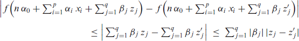
To prove the semi-contractive condition (A2), we utilize the mean value theorem and conclude that $f(x_2)-f(x_1)=f^{\prime }(\xi )(x_2-x_1)$ for some $\xi$ with $x_2>\xi >x_1$ . Since $s{c}_{c^{\prime }}(x)<1$ according to (A2), also $f^{\prime }(x)<1$ such that $f$ is Lipschitz-continuous with constant 1. In particular,

$$\begin{array}{l}\left|f(n{\alpha }_0+{\displaystyle \sum }_{i=1}^p{\alpha }_i{x}_i+{\displaystyle \sum }_{j=1}^q{\beta }_j{z}_j)-f(n{\alpha }_0+{\displaystyle \sum }_{i=1}^p{\alpha }_i{x}_i+{\displaystyle \sum }_{j=1}^q{\beta }_j{z^{\prime }}_j)\right|\\ \le \left|{\displaystyle \sum }_{j=1}^q{\beta }_j{z}_j-{\displaystyle \sum }_{j=1}^q{\beta }_j{z^{\prime }}_j\left|\le {\displaystyle \sum }_{j=1}^q\right|{\beta }_j\left|\right|z_j-{z^{\prime }}_j\right|\end{array}$$

for all $x_i\mathrm{,}{z}_j\mathrm{,}{z^{\prime }}_j$ , so (A2) follows.

A major difference to Weiß et al. (2022) is the argumentation for the similarity condition (A3). Here, Lemmata 21 and 2 allow to conclude that there exists a $\delta >0$ such that

$$TV(Bin(n\mathrm{,}{p}_1)\mathrm{,}Bin(n\mathrm{,}{p}_2))\le 1-\exp (-\delta |p_1-p_2|)$$

holds for the conditional distribution of the scBINGARCH $(p\mathrm{,}q)$ process (2.6). So the proof of Theorem 2.2 is complete.

B.3 Proof of (3.5)

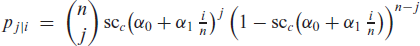
To prove that Condition 5.1 of Billingsley (1961) holds, first note that the set of pairs $(j\mathrm{,}i)$ , where the transition probability

$$p_{j|i}=\left(\begin{array}{c}n\\ j\end{array}\right)s{c}_c{({\alpha }_0+{\alpha }_1\frac{i}{n})}^j{(1-s{c}_c({\alpha }_0+{\alpha }_1\frac{i}{n}))}^{n-j}$$

is truly positive, is independent of the parameter vector $\theta =({\alpha }_0\mathrm{,}{\alpha }_1)$ , because $P_t\in (\mathrm{0,1})$ always holds, and the binomial distribution always has the full support $\{\mathrm{0,}\dots \mathrm{,}n\}$ . Furthermore, the $p_{j|i}$ have continuous (third-order) partial derivatives w. r. t. $\theta$ , because they are a composition of continuously differentiable functions.

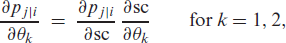
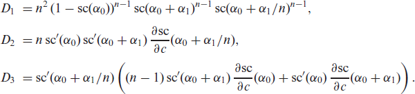
Let us have a closer look at the first-order derivatives. For the sake of readability, we omit the subscript ‘ $c$ ’ in the sequel. Then, we compute

$$\frac{\partial p_{j|i}}{\partial {\theta }_k}=\frac{\partial p_{j|i}}{\partial sc}\frac{\partial sc}{\partial {\theta }_k}\text{\hspace{1em}\hspace{1em}for}k=\mathrm{1,2,}$$

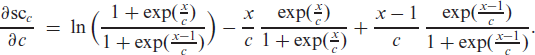
where the partial derivative of $p_{j|i}$ with respect to the soft-clipping function is given by

$$\frac{\partial p_{j|i}}{\partial sc}=\left(\begin{array}{c}n\\ j\end{array}\right)(js{c}^{j-1}{(1-sc)}^{n-j}-(n-j)s{c}^j{(1-sc)}^{n-j-1})\mathrm{.}$$

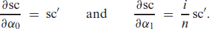
The partial derivatives of the soft-clipping function with respect to $\theta$ , in turn, are

$$\frac{\partial sc}{\partial {\alpha }_0}=sc\text{'}and\frac{\partial sc}{\partial {\alpha }_1}=\frac{i}{n}sc\text{'}\mathrm{.}$$

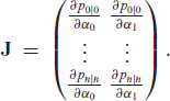
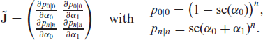
We define the following ( ${(n+1)}^2\times 2)$ Jacobian matrix:

$$J=\left(\begin{array}{cc}\frac{\partial p_{0|0}}{\partial {\alpha }_0}& \frac{\partial p_{0|0}}{\partial {\alpha }_1}\\ ⋮& ⋮\\ \frac{\partial p_{n|n}}{\partial {\alpha }_0}& \frac{\partial p_{n|n}}{\partial {\alpha }_1}\\ & \end{array}\right)\mathrm{.}$$

If this matrix has full rank throughout the parameter space, then Condition 5.1 holds. We consider the following (2 $\times$ 2) quadratic sub-matrix:

$$J=\left(\begin{array}{cc}\frac{\partial p_{0|0}}{\partial {\alpha }_0}& \frac{\partial p_{0|0}}{\partial {\alpha }_1}\\ \frac{\partial p_{n|n}}{\partial {\alpha }_0}& \frac{\partial p_{n|n}}{\partial {\alpha }_1}\\ & \end{array}\right)\text{\hspace{1em}with\hspace{1em}}\begin{array}{l}{p}_{0|0}=(1-sc({\alpha }_0{))}^n\mathrm{,}\hfill \\ p_{n|n}=sc{({\alpha }_0+{\alpha }_1)}^n\mathrm{.}\hfill \\ \hfill \end{array}$$

The determinant of $J$ is given by

$$\det (J)=\frac{\partial p_{0|0}}{\partial {\alpha }_0}\frac{\partial p_{n|n}}{\partial {\alpha }_1}=-n^2\text{\hspace{0.05em}sc}\text{'}({\alpha }_0)\text{\hspace{0.05em}sc}\text{'}({\alpha }_0+{\alpha }_1){(1-\text{sc}({\alpha }_0))}^{n-1}\text{\hspace{0.05em}sc}{({\alpha }_0+{\alpha }_1)}^{n-1}\mathrm{.}$$

Because $0<\text{sc}\mathrm{,}\text{sc}\text{'}<1$ , we have $\det (J)<0$ . Therefore, $J$ and $J$ have full rank, which completes the proof of (2.11).

Additional Estimation of $c$ (Remark 1)

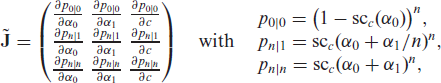
Generally, the previous argumentation could be extended to also cover the adjustment parameter $c>0$ . Since a bivariate Markov chain is fully specified by two model parameters, the upper bound $n$ needs to satisfy $n\ge 2$ if also $c$ needs to be estimated. In addition to the previous derivatives, one now also needs the partial derivative of $s{c}_c$ w. r. t. $c$ , that is,

$$\frac{\partial s{c}_c}{\partial c}=\ln (\frac{1+\exp (\frac{x}{c})}{1+\exp (\frac{x-1}{c})})-\frac{x}{c}\frac{\exp (\frac{x}{c})}{1+\exp (\frac{x}{c})}+\frac{x-1}{c}\frac{\exp (\frac{x-1}{c})}{1+\exp (\frac{x-1}{c})}\mathrm{.}$$

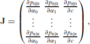
While $0<sc\text{'}(x)<1$ with a maximum in $x=0.5$ , $\frac{\partial sc}{\partial c}(x)$ has a point of symmetry in $(\mathrm{0.5,0})$ : $\frac{\partial sc}{\partial c}(0.5+x)=-\frac{\partial sc}{\partial c}(0.5-x)$ . Next, one defines the ( ${(n+1)}^2\times 3)$ Jacobian matrix

$$J=\left(\begin{array}{ccc}\frac{\partial p_{0|0}}{\partial {\alpha }_0}& \frac{\partial p_{0|0}}{\partial {\alpha }_1}& \frac{\partial p_{0|0}}{\partial c}\\ ⋮& ⋮& ⋮\\ \frac{\partial p_{n|n}}{\partial {\alpha }_0}& \frac{\partial p_{n|n}}{\partial {\alpha }_1}& \frac{\partial p_{n|n}}{\partial c}\\ & & \end{array}\right)\mathrm{,}$$

which needs to be shown to have full rank throughout the parameter space. Again, one may look at appropriate (3 $\times$ 3) quadratic sub-matrices for proving the full rank. For example, the sub-matrix

$$J=\left(\begin{array}{ccc}\frac{\partial p_{0|0}}{\partial {\alpha }_0}& \frac{\partial p_{0|0}}{\partial {\alpha }_1}& \frac{\partial p_{0|0}}{\partial c}\\ \frac{\partial p_{n|1}}{\partial {\alpha }_0}& \frac{\partial p_{n|1}}{\partial {\alpha }_1}& \frac{\partial p_{n|1}}{\partial c}\\ \frac{\partial p_{n|n}}{\partial {\alpha }_0}& \frac{\partial p_{n|n}}{\partial {\alpha }_1}& \frac{\partial p_{n|n}}{\partial c}\\ & & \end{array}\right)\text{\hspace{1em}with\hspace{1em}}\begin{array}{l}{p}_{0|0}=(1-s{c}_c({\alpha }_0{))}^n\mathrm{,}\hfill \\ p_{n|1}=s{c}_c{({\alpha }_0+{\alpha }_1/n)}^n\mathrm{,}\hfill \\ p_{n|n}=s{c}_c{({\alpha }_0+{\alpha }_1)}^n\mathrm{,}\hfill \\ \hfill \end{array}$$

has the determinant $\det (J)=D_1(D_2-D_3)$ with

$$\begin{array}{l}{D}_1=n^2{(1-\text{sc(}{\alpha }_0\text{)})}^{n-1}\text{sc}{({\alpha }_0+{\alpha }_1)}^{n-1}\text{sc}{({\alpha }_0+{\alpha }_1/n)}^{n-1},\\ \begin{array}{l}{D}_2=n\text{sc}\text{'}({\alpha }_0)\text{sc}\text{'}({\alpha }_0+{\alpha }_1)\frac{\partial sc}{\partial c}({\alpha }_0+{\alpha }_1/n),\hfill \end{array}\\ \begin{array}{l}{D}_3=\text{sc}\text{'}({\alpha }_0+{\alpha }_1/n)\left((n-1)\text{sc}\text{'}({\alpha }_0+{\alpha }_1)\frac{\partial sc}{\partial c}({\alpha }_0)+\text{sc}\text{'}({\alpha }_0)\frac{\partial sc}{\partial c}({\alpha }_0+{\alpha }_1)\right).\hfill \end{array}\end{array}$$

Since the first factor $D_1$ is always positive, it remains to show that $D_2-D_3$ is non-zero for the considered paremeter scenario.

B.4 Proof of Theorem 1

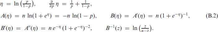
We have to verify the conditions (A0)–(A7) in Davis & Liu (2016). For this purpose, we adapt the notations of Davis & Liu (2016). The distribution $Bin(n\mathrm{,}p)$ belongs to the one-parameter exponential family with

$$\begin{array}{l}\eta =\ln (\frac{p}{1-p})\mathrm{,}\frac{\partial }{\partial p}\eta =\frac{1}{p}+\frac{1}{1-p}\mathrm{,}\hfill \\ A(\eta )=n\ln (1+e^{\eta })=-n\ln (1-p)\mathrm{,}B(\eta )=A^{\prime }(\eta )=n{(1+e^{-\eta })}^{-1}\mathrm{,}\hfill \\ B^{\prime }(\eta )={A^{\prime }}^{\prime }(\eta )=n{e}^{-\eta }{(1+e^{-\eta })}^{-2}\mathrm{,}{B}^{-1}(z)=\ln (\frac{z}{n-z})\mathrm{.}\hfill \end{array}$$

(B.2)

Applied to model (2.14) with $\theta =({\alpha }_0\mathrm{,}{\alpha }_1\mathrm{,}{\beta }_1{)}^{\top }$ , we have the relations

$$M_t=B({\eta }_t)\iff {\eta }_t=B^{-1}(M_t)=\ln (\frac{P_t}{1-P_t})\mathrm{,}{B}^{\prime }({\eta }_t)=n{P}_t(1-P_t)\mathrm{.}$$

(B.3)

Furthermore, the partial derivatives $\frac{\partial }{\partial {\theta }_i}{\eta }_t$ are determined by differentiation of the inverse function $B^{-1}$ :

$$\frac{\partial }{\partial {\theta }_i}{\eta }_t=\frac{1}{B^{\prime }({\eta }_t)}\cdot \frac{\partial }{\partial {\theta }_i}B({\eta }_t)=\frac{1}{P_t(1-P_t)}\cdot \frac{\partial }{\partial {\theta }_i}{P}_t(\theta )\mathrm{.}$$

(B.4)

Let us now check the conditions (A0)–(A7) in Davis & Liu (2016).

• (A0)

  is satisfied because of the parameter restrictions for the scBINGARCH $(\mathrm{1,1})$ process.

• (A1)

  Because of Lemma 2.2, there exist ${ϵ}_1\mathrm{,}{ϵ}_2>0$ such that $P_t\in [{ϵ}_1\mathrm{,1}-{ϵ}_2]$ for all $t$ . Thus, the range $\mathcal{R}(B)$ of $B(\eta )$ has a truly positive lower bound.

• (A2)

  holds because $s{c}_c(x)$ is continuous and, thus, $P_t(\theta )$ is a continuous function of $\theta$ . Actually, $s{c}_c(x)$ is continuously differentiable up to any order, so (A6) also holds.

• (A3)

  does not apply here.

• (A4)

  Because of $P_t\in [{ϵ}_1\mathrm{,1}-{ϵ}_2]$ , also $B^{-1}(M_t)=\ln (\frac{P_t}{1-P_t})$ is a bounded r. v.. So to show (A4), the mean of a bounded r. v. needs to be computed, which necessarily takes a finite value.

• (A5)

  We adapt the argumentation in Appendix C.6 of Davis & Liu (2016). Assume that there is a $t$ such that $P_t(\theta )=P_t(\theta {}^{*})$ almost surely, that is,

  $$s{c}_c({\alpha }_0+{\alpha }_1{X}_{t-1}/n+{\beta }_1{P}_{t-1}(\theta ))=s{c}_c({\alpha }_0^{*}+{\alpha }_1^{*}{X}_{t-1}/n+{\beta }_1^{*}{P}_{t-1}(\theta {}^{*}))\mathrm{.}$$

  Since $s{c}_c(x)$ is injective, $s{c}_c(x)=s{c}_c(y)$ implies $x=y$ , so

  $$({\alpha }_1-{\alpha }_1^{*})X_{t-1}/n={\alpha }_0^{*}-{\alpha }_0+{\beta }_1^{*}{P}_{t-1}(\theta {}^{*})-{\beta }_1{P}_{t-1}(\theta )\mathrm{.}$$

  In particular, $P_{t-1}(\theta )=g(X_{t-2}\mathrm{,}{X}_{t-3}\mathrm{,}\dots )$ and $P_{t-1}(\theta {}^{*})=g^{*}(X_{t-2}\mathrm{,}{X}_{t-3}\mathrm{,}\dots )$ for some functions $g\mathrm{,}{g}^{*}$ , that is, $P_{t-1}(\theta )\mathrm{,}{P}_{t-1}(\theta {}^{*})\in {\mathcal{F}}_{t-2}$ . So with an analogous argumentation as in Appendix C.6 of Davis & Liu (2016), we conclude $\theta =\theta {}^{*}$ .

• (A7)

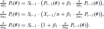
  $B^{\prime }({\eta }_t)$ is bounded by (B.3). Together with Lemma 2.2, it holds that $B^{\prime }({\eta }_t)\in [n{ϵ}_1{ϵ}_2\mathrm{,}\frac{n}{4}]$ . Using (B.4), we compute

  $$E[B^{\prime }({\eta }_t({\theta }_0))(\frac{\partial {\eta }_t({\theta }_0)}{\partial {\theta }_i}{)}^2]=E[\frac{1}{B^{\prime }({\eta }_t)}{(\frac{\partial B({\eta }_t)}{\partial {\theta }_i})}^2]\le CE[(\frac{\partial }{\partial {\theta }_i}{P}_t(\theta {))}^2]\mathrm{.}$$

  Here, with $S_{t-1}=sc{\text{'}}_c({\alpha }_0+{\alpha }_1{X}_{t-1}/n+{\beta }_1{P}_{t-1}(\theta ))\in (\mathrm{0,}\kappa ]$ with $\kappa =sc{\text{'}}_c(0.5)<1$ , we have

  $$\begin{array}{l}\frac{\partial }{\partial {\beta }_1}{P}_t(\theta )=S_{t-1}\cdot (P_{t-1}(\theta )+{\beta }_1\cdot \frac{\partial }{\partial {\beta }_1}{P}_{t-1}(\theta )),\\ \frac{\partial }{\partial {\alpha }_1}{P}_t(\theta )=S_{t-1}\cdot (X_{t-1}/n+{\beta }_1\cdot \frac{\partial }{\partial {\alpha }_1}{P}_{t-1}(\theta )),\\ \frac{\partial }{\partial {\alpha }_0}{P}_t(\theta )=S_{t-1}\cdot (1+{\beta }_1\cdot \frac{\partial }{\partial {\alpha }_0}{P}_{t-1}(\theta )).\end{array}$$

  So each partial derivative satisfies a linear first-order difference equation of the form

  $$\frac{\partial }{\partial {\theta }_i}{P}_t(\theta )=a_{t\mathrm{,}i}+b_{t\mathrm{,}i}\cdot \frac{\partial }{\partial {\theta }_i}{P}_{t-1}(\theta )\text{\hspace{1em}withcoefficients}{a}_{t\mathrm{,}i}\in [\mathrm{0,}\kappa ]\text{and}{b}_{t\mathrm{,}i}\in (-\kappa \mathrm{,}\kappa )\mathrm{.}$$

  Thus, $\frac{\partial }{\partial {\theta }_i}{P}_t(\theta )$ has a bounded range, and (A7) holds.

Supplementary materials

Supplementary materials for this article are available online.

Supplemental Material for Soft-clipping INGARCH models for time series of bounded counts by Christian H. Weiß, Malte Jahn, in Statistical Modelling