
Abstract
Recurrent events analysis plays an important role in many applications, including the study of chronic diseases or recurrence of infections. Historically, many models for recurrent events have been variants of the Cox model. In this article we introduce and describe the application of the piece-wise exponential Additive Mixed Model (PAMM) for recurrent events analysis and illustrate how PAMMs can be used to flexibly model the dependencies in recurrent events data. Simulations confirm that PAMMs provide unbiased estimates as well as equivalence to the Cox model when proportional hazards are assumed. Applications to recurrence of staphylococcus aureus and malaria in children illustrate the estimation of seasonality, bivariate non-linear effects, multiple timescales and relaxation of the proportional hazards assumption via time-varying effects. The R package
Keywords
Introduction
A recurrent events setting in survival analysis is defined by repeated observations of an event of interest over the course of the observation period. In medical, clinical and biological research, such data play an important role, for example, in the context of chronic illnesses and infectious diseases. Some concrete examples include recurrence of hospitalization for cardiovascular events (Gibson et al., 2017; Varma et al., 2021), recurrent diseases and infections like COVID-19 (Dos Santos et al., 2021), pneumonia (Ramjith et al., 2021; Barakat et al., 2021), pneumococcus (Hernstadt et al., 2020), staphylococcus aureus (cf. Section 5.1) (Akinboyo et al., 2018; Abdulgader et al., 2019), asthma (Chan et al., 2021; Feng et al., 2021) and malaria (cf. Section 5.2) (Lawpoolsri et al., 2019; Ghosh et al., 2020; Kakuru et al., 2020).
Typical for this kind of data are the correlations, or more generally dependencies, between event recurrences. Such dependencies may be induced by an individual-specific unmeasured frailty, common across all events of the individual, or by dependence of the occurrence of an event on an individual’s history. In the latter case the hazard of an event could depend on the timing (e.g., time since last event) or the frequency (number of previous events). Ignoring either type of dependency, if present, leads to biased estimates or overoptimistic standard errors (Box-Steffensmeier and De Boef, 2006; Jahn-Eimermacher, 2008). To choose an appropriate model for the analysis of recurrent event data, assumptions on this dependency structure must be made as well as a choice on the timescale for the analysis of events: gap time (also referred to as waiting time, clock-reset or renewal approach) or calendar time (clock-forward). See Section 2.1 for more discussion about the timescale.
Several recurrent events models for calendar and gap times have been suggested in the literature. These models attempt to account for the effects of within-subject correlation either by adjusting the variances of the parameter estimators (the variance-adjustment models (Andersen and Gill, 1982; Prentice et al., 1981)) or by including a subject-specific random effect in the model—the shared frailty model (SFM). Variance-adjustment models assume independence among events when estimating the effect of the covariates, while adjusting the standard errors of the parameter estimates for the correlation between recurrent events by calculating robust variance through sandwich estimation (Huber, 1967; Freedman, 2006). SFMs (Hougaard, 2012) account for correlated events within an individual (and thus heterogeneity in the sample) by adding individual specific random effects, which act in a multiplicative way on the hazard function. In this work, we focus on the frailty (or random effects) model. In a standard SFM it is assumed that the hazards are proportional over time (conditional on the random effect) and the baseline hazard function is unspecified (in the Cox SFM), but a parametric form may be chosen as well. For interpretation of the estimated effects, an estimate of the baseline hazard function is important. Putter et al. (2005) mentioned that not knowing the baseline implies that the risk of observing an event at particular points in time remains unknown. The importance of knowing the absolute risk (or baseline hazard) when interpreting relative risks is further highlighted by Noordzij et al. (2017). They suggest that readers tend to overestimate or over-interpret relative risks when information about the absolute risks is missing. This is even strengthened if the hazard ratio is expected to be time-dependent. An understanding of the baseline hazard over time is important for clearer interpretation of time-varying effects (Ruhe, 2018).
Many publications on recurrent events analysis focus on variants of the Cox proportional hazards (CPH) model (Cox, 1972). This includes the SFM, mentioned earlier, and the variance-adjustment models, specifically the Andersen-Gill (AG) model, the Prentice-Williams-Peterson (PWP) models, and the Wei, Lin and Weissfeld (WLW) model (Andersen and Gill, 1982; Prentice et al., 1981; Wei et al., 1989). The AG model estimates a common baseline hazard for all events and covariate effects are usually estimated across events as well. In the PWP and WLW models the baseline hazards are stratified for the different events, and covariate estimates are either estimated across events or event-specific. The PWP models are constructed in either a calendar time approach or a gap time approach (see Section 2.1), while the WLW model is constructed using marginal times (where the time at risk for each event is counted from the study start). In the AG and PWP models, individuals only remain at risk for the event following their last observed event, while for the WLW model, individuals remain at risk for the maximum number of observed events. Studies (Kelly and Lim, 2000; Therneau and Hamilton, 1997) have shown a carry-over effect when using the WLW model and recommend that it can be used for modelling multiple event types rather than recurrent events. There are several tutorials available with applications and comparisons of these methods (Kelly and Lim, 2000; Therneau and Hamilton, 1997; Amorim and Cai, 2015; Ullah et al., 2014), and a recent tutorial on SFMs is provided by Balan and Putter (2020).
Parametric SFMs can be a useful alternative to the semi-parametric SFM. In the parametric SFM the baseline hazards can be modeled through a choice of many parametric distributions each with its own characteristics (Munda et al., 2012). Misspecification of the baseline hazards can lead to bias in estimated effects and possibly misleading results for the shape of the hazard function (Hutton and Monaghan, 2002; Kwong and Hutton, 2003; Li et al., 1996). In a recurrent events setting where the shape of the baseline hazard differs, for example between first and recurrent events, a mixture of parametric models must be used to appropriately capture the baseline hazards (Duchateau et al., 2003). This can be a complicated task.
More flexible models like the generalized survival models (GSMs) (Liu et al., 2017) are becoming increasingly more popular in modelling the baseline hazards. These models use a smoothing splines approach and allow more complexities such as time-dependent effects, nonlinear effects, and their interactions. The GSM has recently been extended to model correlated survival data: SFMs with time-constant covariates for gap time formulations or an AG variance-adjustment type model for calendar time formulations. However, GSMs still needs to be extended to SFMs in a calendar time framework.
Here we introduce the Piece-wise exponential Additive Mixed Model (PAMM) (Bender et al., 2018; Argyropoulos and Unruh, 2015) for modelling possibly time-varying effects, nonlinear effects and more complex interactions in a recurrent events setting where it is possible to consider multiple time scales, stratified baseline hazards and time-varying covariates. As the Cox model, PAMMs model the hazard rate without parametric assumptions about the distribution of event times and multiplicative covariate effects. Thus, if model specification is equivalent, both models lead to similar results and interpretation.
While conceptually similar to the Cox model, PAMMs offer an alternative method for survival analysis that has recently gained popularity. This is mainly due to the fact that PAMMs reformulate many different survival tasks to regression tasks via a data augmentation step and availability of software that facilitates practical application (Bender and Scheipl, 2018). While this allows the model to be estimated by any algorithm that can optimize the Poisson likelihood (Bender et al., 2021), the Generalized Additive Mixed Model (GAMM) framework has proven to be particularly useful, due to its flexibility, availability of robust and established estimation techniques (e.g., Hastie and Tibshirani (1986); Wood (2017)) and interpretability of covariate effects. This allows great versatility in modelling choices, as discussed in more detail in Section 6. In particular, PAMMs facilitate seamless estimation of multivariate, non-linear, time-varying effects via penalized splines with different basis functions, cyclic splines and splines with shape constraints (Pya and Wood, 2015). Recent examples include spline based stratified baseline hazard estimation in plant biology (Panel et al., 2020), cumulative effects in critical care (Bender et al., 2019), treatment effects with non-proportional hazards in patients with coronary stent restenosis (Giacoppo et al., 2020), estimation of bivariate effect surfaces in the context of randomized controlled trials (Argyropoulos and Unruh, 2015) and progression-free survival in patients with gastroenteropancreatic neuro-endocrine tumors (Carmona-Bayonas et al., 2019), and time-varying hazard ratios in post-transplant outcome assessment (Wey et al., 2020). An application to the recurrence of childhood pneumonia was recently presented in Ramjith et al. (2021). In general, however, detailed instructions on the application of PAMMs to survival tasks, especially tasks that go beyond the single-event setting with right-censoring as well as software tools that facilitate such analyses, particularly recurrent events analyses, are scarce.
In this article we give an introduction to PAMMs for recurrent events analysis. This includes data transformation specific to recurrent events and discussion on the choice of timescale. We show that the model performs well and generates unique insights by means of simulation studies and real data examples. The article is accompanied by the R package
In the remainder of this work, we summarize hazard based model specification and estimation for recurrent events analysis in Section 2. In Section 3, we show how such models can be estimated using PAMMs, including a step by step guide on the necessary data augmentation. A comparison of the SFM and the PAMM when proportional hazards are assumed (conditional on the frailty) is made through a simulation study in Section 4. Section 5 concludes with examples of PAMMs applied to different recurrent events data sets and illustrates effect estimation of different complexities, that is, stratified baseline hazards, non-linear, cyclic effects of seasonality and multiple timescales. We conclude with a discussion and an outlook in Section 6.
Models for recurrent events
Timescale
The choice between the two timescales (gap time or calendar time) is usually driven by the research setting in which the data are collected, and the research question at hand, as the choice of the timescale affects the interpretation of the results (see Duchateau et al., 2003; for a thorough discussion). On both timescales, the study start time needs to be clearly defined and meaningful, for example, time from birth, time from randomization, time from diagnosis. Calendar time is appropriate when the interest is in the full course of the recurrent event process. On this timescale an individual’s time starts when entering the study and stops when leaving the study. For the first event, the individual’s contribution to time at risk is counted from entering the study. However, the individual’s contribution to time at risk for the second event is only counted from the first event, the start time of the risk interval for the second event. A calendar time data set can be viewed as a succession of (internally) left-truncated data sets for each of the events, as a subject’s time at risk is left-truncated at the event time of the previous event.
In the gap time approach one is interested in the time between events. Essentially, that means that after every event ‘the clock’ is reset; after each event the time since the previous event is used to define time intervals that an individual is at risk for an event. Thus, in contrast to the calendar time approach, a subject is at risk for all of his events at time t = 0, however, time to event is redefined as time from last event to next event. Historically, the gap time approach facilitates analysis, because the data could be evaluated with standard techniques for survival analysis without the need to take into account left-truncation. Assuming a full renewal process, all observations are considered independent. Dependence induced by number of previous events can be modeled by stratifying the hazards by event number. Dependence introduced by within-subject correlation can be modeled by introducing a frailty term.
In the PAMM framework, the choice of timescale is less important, as we can always add additional time-dependent covariates to describe the past. In calendar time, for example, we could include a variable for the gap time of the previous event or the number of previous events. In the gap time approach, we can include dependence on the total time since entering the study, and so on. More generally, PAMMs support dependence on multiple timescales (Iacobelli and Carstensen, 2013), as any dependence on time is modeled through covariate effects of different representations of time.
Model speciftcation
In the following we consider models for the (conditional) hazard function for the k − th event for subject i given by

where, t is the time of interest,

Assuming a common baseline hazard for all events, the model could be further simplified by replacing λ0,k with λ0, resulting in the so-called unstratified (or unconditional on episode order) SFM (Hougaard, 2012).
The conditional likelihood for model 2.1 in calendar time (given the individual frailty terms) is proportional to

where Ki is the number of events for which subject i was at risk, ti,k the event time for event k for k < Ki, ti,Ki is the time subject i was censored, and ti,0 the entering time for subject i which is usually equal to 0. Furthermore, δi,k is the event specific status indicator, so δi,k = 1 for k < Ki and

The likelihood functions given so far are conditional the frailty variable. The marginal (unconditional) likelihood function is proportional to

where fZ is the density function of the frailty variable.
The likelihood for the gap time model (conditional on frailty) is equivalent to 2.2 with ti,k replaced by

Data augmentation and estimation
As described in detail elsewhere (Bender et al., 2018), application of PAMMs to time-to-event data requires a particular data augmentation step. We refer to the resulting data as piece-wise exponential data (PED). In principle, the data augmentation required for recurrent events analysis is equivalent, however, some specifics need to be taken into account, that also depend on the timescale of the analysis.
As for the single-event PED, the follow-up has first to be discretized into J intervals with cutpoints
Let

where i = 1, ..., n the subject identifier as before, j = 1, ..., J denotes the interval and k = 1, ..., K the event number. Thus, δijk indicates whether subject i, experienced an event of type k in interval j (1=yes, 0=no) and tijk is the time for which subject i was at risk for the kth event in interval j. Note that for a particular subject i we only calculate these variables for time points (intervals) at which they were at risk for the particular event number. Doing so also naturally accounts for left-truncation at the beginning of the follow up as well as left-truncation for recurrent events on the calendar timescale (induced by the recurrent events process).
Consider a specific event k. Assuming piece-wise constant hazards

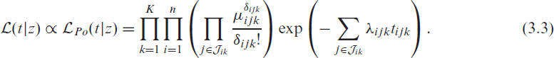
in each interval, the likelihood contribution of subject i (conditional on the frailty variable) in 2.2 can be rewritten as

where
Similar to 2.4, the conditional likelihood in 3.3 can be expressed as a marginal likelihood by specifying a frailty distribution:
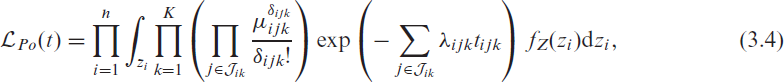
where
The reformulation of recurrent events models into Poisson regression models is interesting especially due to flexibility of GAMMs and readily available software. In PAMMs we parameterize the interval- and event-specific hazard rates 3.1 via (non-linear) covariate effects. An exemplary model specification is given below:

In 3.5,
From an estimation and inference perspective, the model is a Poisson regression task with additive and random effects. Therefore, the parameters of the model can be estimated by optimizing the penalized Poisson likelihood 3.6 using the GAMM framework (e.g., Wood, 2017).
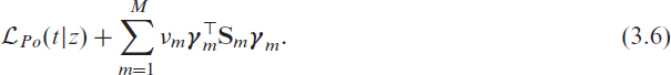
In 3.6, M is the total number of smooth and random effects in the model and νm the respective penalty parameter estimated from the data;
Joint optimization of all parameters in 3.6 can be done in different ways. In the application section, we use the methods implemented in package
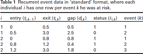
Exemplary recurrent time-to-event data for two individuals,
Recurrent event data in ‘standard’ format, where each individual i has one row per event k he was at risk.
Recurrent event data in ‘standard’ format, where each individual i has one row per event k he was at risk.
In Table 1 the unique event-specific gap times, ordered with respect to length, are given by 0.4, 0.5, 0.8 (values from column di,k in Table 1 with δik = 1). The maximum gap time is 2.5, however, it usually makes sense to set interval border of the last interval J to the maximum event time, which is 0.8 in this example as there is no information about event times beyond that point. Therefore we will use cutpoints (0,0.4,0.5,0.8) and the intervals in this example will be defined as

The transformation of Table 1 to the PEM data format based on these intervals is shown in Table 2.
Recurrent event data in PEM data format on the gap timescale.
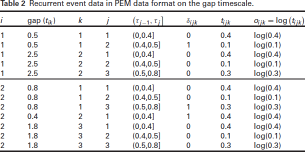
Recurrent event data in PEM data format on the gap timescale.
On the calendar timescale we consider the ordered time points at which an event took place (or end of study) 0.5, 0.8, 1.2. Once again, we do not consider time points beyond the last observed event time. Next, we split the follow-up into intervals using these time points as cutpoints:

The resulting data in the piece-wise exponential format is given in Table 3.
Recurrent event data in PEM data format on the calendar timescale.
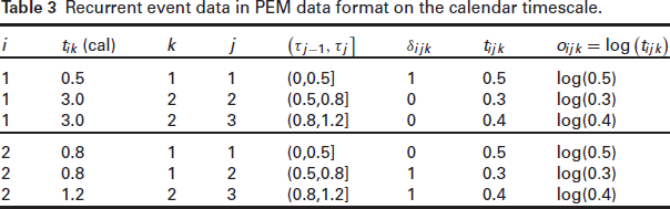
Recurrent event data in PEM data format on the calendar timescale.
Comparison of PAMM and SFM in a proportional hazards setting
Under the assumption of proportional hazards the proposed PAMM and the SFM should give similar estimates of the regression parameters and the frailty variance. In order to check whether this is true an extensive simulation study was performed. The simulation settings as well as the simulation results are given in Supplement 1. In summary, it is shown that under the proportional hazards assumption the PAMM and the SFM give (almost) identical results for the estimated regression parameters in both gap- and calendar timescales, using the stratified and/or unstratified models. Furthermore, both models tend to estimate the regression parameters and the frailty variance more accurately when there is a longer follow-up time or there are more recurrences. It must be noted that when the frailty variances are large both models underestimate the frailty variance, but this underestimation is lower for longer follow-up times. Specifically, in the gap time scenarios, we see that the underestimation is worse in the SFM, and in the calendar time scenarios the underestimation is worse in the PAMM. The consequences of these biases of the estimated frailty variance on the estimates of the regression coefficients are minimal. It should be noted that the varying results for the frailty variances could depend on model implementation, and not necessarily on the model formulation, where
Comparison of PAMM and SFM in distinguishing frailty and time-varying effects
Balan and Putter (2019) showed in simulation studies that in certain scenarios of clustered survival data – including recurrent events, it is difficult to distinguish the presence of a frailty effect from the presence of a time-varying effect. We replicated their simulation study for recurrent events to compare how the PAMM and the SFM distinguishes between a frailty effect and a time-varying effect. The only difference is that we used log-normal frailties for the Cox-like SFM, since the implementation of PAMM using
Motivating examples
In this section we apply the PAMM for recurrent events to two real-life data sets using R (R Core Team, 2020; RStudio Team, 2020). We use the R packages
Example 1: Staphylococcus aureus infection data
The staphylococcus aureus (SA) infection data in Abdulgader et al. (2019) contains times at which 137 children were colonized with a new staphylococcus aureus infection in the nasopharynx in their first year of life in Paarl, South Africa. In Abdulgader et al. (2019), the gap time PWP model (Prentice et al., 1981) was used to model the survival curves for the different infections (i.e., first, second, third, etc.). A standard CPH model was also used to investigate the effects of risk factors on the time to the first infection. In this section, we aim to repeat their analysis but include recurrent infections using the stratified PAMM (see equation (3.5)) in gap time. We consider a different baseline hazard for the first event and for recurrent events (combined). An advantage of using the PAMM here is that we can easily model, estimate and visualize the baseline hazards stratified for the first and recurrent events. We use the HIV exposure variable, where some children are HIV exposed and uninfected (HEU) and the rest are HIV unexposed (HU). First we look at the baseline hazards and then we look at a proportional hazards model for HIV exposure where the effect of HIV exposure is different for first and recurrent events.
Baseline hazards
We first fit the model without the HIV covariate but including the frailty term (i.e., λ(t) = λ0 ,k (t) exp (zi)) to have an understanding of the functional form of the baseline hazard. The estimated frailty variance is 0.066 (p = 0.249). This is a small frailty variance and so we will exclude the frailty term and reduce our model to a simpler model.
The estimated degrees of freedom, explained in Supplement 2, for the evolution of the hazard rate over time is different for first and recurrent SA infection, indicating that the evolution of the baseline hazards for first and recurrent events may be different (note: we are not testing for a difference in the baseline hazards). We visualize the estimated baseline hazard in Figure 1, where the hazard rates are re-scaled to correspond with the number of events per child-year. For the first SA event, the hazard rate is highest after birth and decreases quickly until around 5 months, thereafter a very slow decline is seen. For recurrent SA infections, we see an increase in the hazard over time since the previous infection until about three months. Thereafter we see an almost constant hazard for a recurrent infection and a slow decline starting from around 9 months.
The hazard rates for (A ) first and (B ) recurrent SA infections respectively. 95% confidence intervals are shaded in gray.
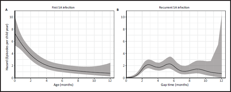
The hazard rates for (A ) first and (B ) recurrent SA infections respectively. 95% confidence intervals are shaded in gray.
The hazard function of the model we are interested in, is

where
In the paper by Abdulgader et al. (2019), the univariable analysis of HIV exposure on the time to first SA infection showed a HR effect close to 1. Next, we model an interaction of HIV exposure and the recurrence indicator to allow a separate HIV exposure effect for first and recurrent events, that is,

where
To illustrate application of PAMMs on calendar timescale, we reanalyze data from a study of childhood malaria undertaken by (Kakuru et al., 2020) in Uganda to study the effects of two intermittent preventive treatments, with Sulfadoxine-pyrimethamine (SP) and Dihydroartemisininpiperaquine (DP) on the incidence of childhood malaria from birth until children are one year old. Therefore, the timescale for events and recurrences coincides with the age of the children in this example. In the original analysis, treatment effect was investigated with respect to the time to first episode of malaria, and it was found that there may be larger treatment differences between boys but not between girls. Here we analyze time to first event and additionally recurrences and add preterm birth and gravidity (number of previous pregnancies) as additional risk factors in the model. We further illustrate incorporation of cyclic splines and bivariate smooth functions by incorporating a seasonal effect and later its interaction with child age. An advantage using PAMMs, similar to Example 5.1, is that the baseline hazards are flexibly estimated, while simultaneously estimating a non-linear effect of seasonality, all in a SFM setting. Furthermore, it can easily be investigated, through more complex interactions, if there is any indication of the non-linear seasonality effect changing over time). Additionally in Supplement 3 we show the effects of different choices of basis functions for the baseline hazards, as well as degrees of freedom.
Model specification
We fit the following model
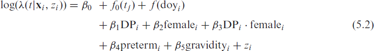
where
The results show a significant frailty variance (
The results of the analysis show a significant treatment effect for boys, where DP is associated with a lower hazard of malaria over time compared with SP (
The estimated non-linear effects of age and seasonality are depicted in Figure 2. The upper row shows the effect of the child’s age as log-hazard contribution of the non-constant baseline term f0(tj) (left panel) and as hazard/incidence rates (episodes per child year) (right panel). The hazard rates were calculated by using varying time values while holding all other covariate values constant.
Upper row: The non-constant part of the log-baseline (f0(t)) including confidence intervals (left panel) and respective hazard/incidence rates (episodes per child year, other covariate held constant; right panel) across age. Bottom row: Effect of seasonality as contribution to the log-hazard (f (doy), left panel) and hazard/incidence rates (episodes per child year, given child of age 100 days, other covariates as before; right panel).
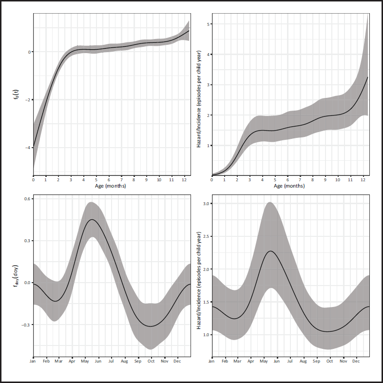
Specifically, doy=1, treatment=DP, sex=Female, preterm=no and gravidity=1. From both graphs, we can see that the hazard of contracting malaria rises quickly as children get older until approximately 3 months of age, where the effects starts to level off. The bottom row of Figure 2 depicts the seasonality of malaria infection, where once again, the left panel depicts the log-hazard contribution of the term f (doy) and the right panel the hazard/incidence rates (episodes per child year, for children of varying levels of seasonality, 100 days of age, other covariates fixed as before). They show that the hazard rates go up from the start of the rainy seasons (January) and start to go down from the start of the dry seasons, with the second rainy season of the year (around June) showing a larger effect on the hazard of malaria. Per construction, the effect is the same at the end of December as in the beginning of January.
As children get older, they might be left unattended for longer periods of time and potentially spent more time outside or otherwise unprotected (e.g., by nets). We therefore additionally investigate a potential interaction between child age and seasonality when it comes to the hazard of malaria infection, for example such that seasonality does not affect the hazard for very young children as much as for older children. Since both variables are continuous, we model the interaction via bivariate penalized splines represented by tensor products, such that Equation 5.2 becomes

Note that in Equation 5.3 the non-linear part of the baseline hazard is now a function of both, age (tj) and day of year (doy). This term can thus be viewed as a time-varying effect of the day of year, as it depends on tj. In this case, however, it can also be viewed as an example for the application of multiple timescales, as the hazard depends on age (time since origin) and the day of year (calendar time).
The estimated bivariate effect f0(tj, doy) is depicted in Figure 3 (as before, similar representations could be obtained for the hazard/incidence rate where the other covariates are fixed at selected values). The left panel shows the surface of the bivariate function, with brighter colours indicating larger hazards. The middle panel shows vertical slices through the surface for fixed values of age, while the right panel shows horizontal slices through the surface for fixed values of day of year (season). These results are in line with the results obtained from model 5.2 and in this case indicate, that there is no substantial interaction between child age and seasonality effect. This conclusion could also be obtained more formally, using a ANOVA type decomposition of the bivariate effect into main and interaction effects (Wood, 2006), as illustrated in Suppplement.
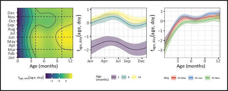
Note: Brighter colors indicate increased hazards. Horizontal and vertical dashed lines indicate slices through the surface shown in the mid and right panel respectively. Mid panel: Slices through the bivariate surface for child ages 1, 4 and 10 months. Right panel: Slices through the bivariate surface at 1 March, 1 June and 1 November for the day of the year.
In this article we introduced PAMMs as an alternative modelling approach for recurrent events data. These models utilize the generalized additive mixed modelling framework for estimation and inference. This facilitates specification and estimation of models for recurrent event data with complex covariate effects, including (multivariate) non-linear effects, time-varying effects and covariates, multiple timescales as well as random effects. We illustrated the application of PAMMs and specification of different covariate effects on real data sets.
In simulation studies we have shown that in the proportional hazards setting, SFM PAMMs give similar results to the Cox SFM with respect to the estimated effects and frailty variance. In certain scenarios of clustered survival data (including recurrent events) it is difficult to distinguish between unobserved heterogeneity and time-varying effects (non-proportional hazards) in the SFM, especially for smaller cluster sizes (where a cluster size of one implies univariate survival data) (Balan and Putter, 2019). Such identifiability issues result from the data generating process and will persist independently of the model class chosen for the analysis of such data. However, from our simulation study in Supplement 4, we saw that the PAMM has a lower type 1 error rate for detecting a frailty effect in the presence of time-varying effects, even for clusters as small as size two, compared with the Cox SFM. This difference is much more pronounced for larger sample sizes. Also notable in the simulation results, the PAMM may be subject to inflated type 1 errors when used for testing time-varying effects, regardless of whether or not there is unobserved heterogeneity. This simulation study was however limited to a single binary covariate, monotonic shapes of the baseline hazards and without stratification. A considerable amount of work, possibly in terms of a much larger simulation study with a focus on recurrent events, must be carried out to assess these preliminary findings more carefully.
Compared to parametric SFMs, SFMs estimated by PAMMs do not make any assumption about the distribution of event times. Compared to Cox based SFMs, PAMMs directly model the (baseline) hazard via penalized splines. Thus, while for Cox models (and piece-wise exponential models for that matter) the hazard can have implausible jumps between two subsequent time points, PAMMs enforce a penalty on large differences between hazards from neighboring time points (intervals), leading to stable and more plausible hazard estimates.
While PAMMs offer a flexible framework for recurrent events analysis, some readers might be concerned with the expansion of the data set that results from the data augmentation step and, consequently, the computation time. In our experience this is rarely an issue. Especially for small and medium sized data sets, the computation time is barely noticeable (even when using all unique event times as cut-points). For example, on a standard laptop with Intel core-i7 CPU with 1.90GHz, 16GB RAM, fitting the interaction model in Section 5.1 (Equation (5.1)) takes about 1 second; the model estimating incidences of Malaria infection (with bivariate effects, Equation (5.3)), in Section 5.2, takes about 10 seconds. For high-dimensional data efficient estimation methods exist (Wood et al., 2017; Greven and Scheipl, 2020). For models on the gap timescale, computation time could be further improved without sacrificing predictive performance by reducing the number of interval cut points (cf. complexity analysis in Bender et al., 2021).
The R package
Another advantage of the PAMM framework is that it does not require any particular implementation in order to estimate the model. While
A current limitation of these techniques and respective implementations is that they are limited to modelling Gaussian distributed random effects, while Gamma distributed random effects are popular in the context of survival analysis (Balan and Putter, 2020). However, through simulation studies by Gasparini et al. (2019); Liu et al. (2017), it has been shown that the estimates of the regression coefficients are quite robust to misspecification in the choice of frailty distributions regardless of sample size or the amount of heterogeneity as determined by the frailty variance. Gasparini et al. (2019) showed that it is more important to prioritize modelling the baseline hazard correctly. Alternatively, package
This work highlights the usefulness and possibilities of extending PAMMs to recurrent events data.In future research, this model class could be further extended to settings with multivariate recurrent events (i.e., when multiple time-to-event outcomes can (re)occur on the same observation unit), recurrent events data with a terminal or competing event or for recurrent events data with non-zero time to recovery.
Availability of data and materials
Data for the Staphylococcus aureus example are contained within the
Supplementary material
Supplementary material is available online.
Supplemental Material for Recurrent events analysis with piece-wise exponential additive mixed models by Jordache Ramjith, Andreas Bender, Kit C. B. Roes, Marianne A. Jonker, in Statistical Modelling
Footnotes
Acknowledgements
We thank Shima Mohammed, Mark Nicol and Heather Zar for access and support to use the staphylococcus aureus infection data from the Drakenstein Child Health Study. We also thank Abel Kakuru, Grant Dorsey and the rest of the authors in the Uganda malaria birth cohort study for access and support to use the data for secondary analysis. We would also like to thank Theodore Balan for sharing his simulation code, so that we could replicate the simulations for our own comparisons. Lastly we would like to thank the reviewers for their thorough feedback and suggestions.
Declaration of conflicting interests
The authors declared no potential conflicts of interest with respect to the research, authorship and/or publication of this article.
Funding
AB was funded by the German Federal Ministry of Education and Research (BMBF) under Grant No. 01IS18036A.
References
Supplementary Material
Please find the following supplemental material available below.
For Open Access articles published under a Creative Commons License, all supplemental material carries the same license as the article it is associated with.
For non-Open Access articles published, all supplemental material carries a non-exclusive license, and permission requests for re-use of supplemental material or any part of supplemental material shall be sent directly to the copyright owner as specified in the copyright notice associated with the article.