
Abstract
We consider a parametric modelling approach for survival data where covariates are allowed to enter the model through multiple distributional parameters (i.e., scale and shape). This is in contrast with the standard convention of having a single covariate-dependent parameter, typically the scale. Taking what is referred to as a multi-parameter regression (MPR) approach to modelling has been shown to produce flexible and robust models with relatively low model complexity cost. However, it is very common to have clustered data arising from survival analysis studies, and this is something that is under developed in the MPR context. The purpose of this article is to extend MPR models to handle multivariate survival data by introducing random effects in both the scale and the shape regression components. We consider a variety of possible dependence structures for these random effects (independent, shared and correlated), and estimation proceeds using a h-likelihood approach. The performance of our estimation procedure is investigated by a way of an extensive simulation study, and the merits of our modelling approach are illustrated through applications to two real data examples, a lung cancer dataset and a bladder cancer dataset.
Keywords
Introduction
Standard survival analysis models such as the proportional hazards (PH) model are known to have a single covariate-dependent parameter, the scale parameter. As a means to extend these models and afford more flexibility in the modelling of survival data, Burke and MacKenzie (2017) developed a multi-parameter regression (MPR) approach for a parametric hazard function. MPR is an approach whereby more than one distributional parameter is allowed to depend on covariates, and this is sometimes referred to as ‘distributional regression’ (Stasinopoulos et al., 2018; see also Rigby and Stasinopoulos, 2005, and Stasinopoulos et al., 2007). Using the Weibull MPR model as an example, Burke and Mackenzie’s (2017) paper demonstrates the advantages of allowing both the scale and the shape parameters to depend on covariates simultaneously. More recently, Burke et al. (2019) extended a semi-parametric accelerated failure time (AFT) model to multiparameter regression and Burke et al. (2020) explored a parametric MPR survival modelling framework in which the baseline hazard function follows an adapted power generalized Weibull (APGW) distribution.
Standard MPR models rely on the assumption of independent event times, and such an assumption cannot be met in studies with clustered observations. This includes studies where successive or recurrent event times are recorded on each subject; multi-centre studies where survival times of individuals from the same centre may be dependent due to centre-specific conditions, clinical or otherwise; family studies; and matched pair studies. Various methods have been developed to model the lack of independence in clustered data, but perhaps the most standard approach is the one whereby a cluster-specific random effect is introduced into the model. Given these random effects, the data are assumed to be conditionally independent. In the context of survival analysis, such random effects models are commonly referred to as frailty models, and, since the random effect represents a common effect on all members in a cluster, these types of common risk models are known as shared frailty models (Clayton, 1978; Duchateau and Janssen, 2008; Hougaard, 2012).
Extensions of the MPR models to include random effects have been centred around the ‘classical’ multiplicative frailty model, whereby the frailty term is included in the linear predictor corresponding to the scale parameter. Peng et al. (2020) extend a Weibull MPR model for interval censored data to include a gamma distributed multiplicative frailty term, but only for univariate frailty. In their article, Jones et al. (2020) extend the MPR PGW and MPR APGW models to handle bivariate data using multiplicative frailty, where the dependence is understood using links to the well known power variance copula (Goethals et al., 2008; Duchateau and Janssen, 2008; Hougaard, 2012). The attraction of MPR modelling is the flexibility afforded by allowing the hazard shapes to differ, but just as the shape can vary according to covariates, so too could it have random variation, for example, resulting from differences across multiple centres. Hence, in this article, we go beyond the classical multiplicative model to allow for a wider range of model structures: specifically, models in which a frailty term is included in each distributional parameter. This, we believe, is a more natural way of modelling correlated data using MPR models than multiplicative frailty which relates only to the scale of the hazard. Furthermore, our proposed model accounts for the potential correlation between the frailty terms themselves since scale and shape effects may be correlated.
Parameter estimation in the parametric shared frailty model is commonly achieved through integrating out the frailties from the conditional survival likelihood. The resulting equation is an explicit expression for the marginal likelihood, containing the fixed parameters and no longer the frailties. This marginal likelihood can then be maximized using numerical methods to yield estimates for the fixed effects. Inference about the random effects is not readily available and integrating out the frailties from the joint density typically involves the evaluation of analytically intractable integrals over the random-effect distributions. Numerical integration methods such as the Gauss-Hermite (G-H) quadrature can be used to approximate the value of the integrals, however, when the dimensionality of the integral is high, the number of quadrature points grows exponentially with the number of random effects and the approximation is sub-optimal. While several methods, such as the Monte Carlo Expectation-Maximisation, Markov Chain Monte Carlo and Gibbs sampling have been used to overcome the issue of intractable integrals, these methods are notoriously known for being computationally intensive. This is especially true when the number of random effects (clusters) is large or when the complex correlation structure among the clustered survival times requires the assumption of multiple frailties (Vaida and Xu, 2000; Ripatti and Palmgren, 2000; Abrahantes et al., 2007; Duchateau and Janssen, 2008). We adopt a so-called ‘hierarchical likelihood’ (h-likelihood) approach. This approach was originally proposed by Lee and Nelder (1996) for a generalized mixed-effects model but further studied and developed to provide a straightforward, unified framework for various random effect models including frailty models (Ha et al., 2001, 2002; Ha and Lee, 2003; Ha et al., 2017).
In contrast to the standard marginal likelihood approach, the h-likelihood framework treats the random effects or frailties as model parameters, which are then jointly estimated with the fixed parameters and the frailty dispersion parameter(s). Estimates of the fixed and random effects are found by maximizing the log-likelihood function conditional on the random effects plus a penalty term whose value depends on how dispersed the random parameters are: if the random effects have a large dispersion parameter, then the penalty term takes a small value. By treating the random effects as model parameters, the h-likelihood framework avoids the intractable integration needed to calculate the marginal likelihood and provides an efficient estimation procedure. Furthermore, classical analysis of random effects models focuses on the estimation of the fixed parameters and the frailty variance parameter(s), but in many recent applications, estimation of the random effects is also of interest. Such estimates allow for the survivor function for individuals with given characteristics to be estimated the cluster specific failure time distribution—and are especially useful in multi-centre studies when the frailty term represents the centres. Estimates of the random effects in such studies provide information about the merits of the different centres in terms of patient survival and are useful for investigating the potential heterogeneity in survival among clusters in order to better understand and interpret the variability in the data (Ha et al., 2016b).
The remainder of this article is organized as follows: Section 2 describes the MPR model, its extended version with random effects and the h-likelihood procedure for parameter estimation in the given model. Section 3 presents results of extensive simulation studies. The proposed methods are illustrated on two datasets arising from multi-centre studies in Section 4, followed by a discussion and conclusion in Section 5.
The MPR Frailty model
Model formulation
To formulate a shared frailty MPR model for survival data, we assume time-to-event data arising from a multi-centre study. In this study, we have q centres or clusters, with ni individuals (patients), i = 1, 2, 3,...,q. The total sample size is the total number of individuals coming from all q centres, that is,

where
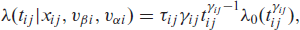
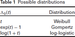
Possible distributions
The two distributional parameters, 
where
In their work, Burke and MacKenzie (2017) found the distributional parameters in an MPR model to be highly correlated. To account for the possibility of the propagation of this correlation to the corresponding frailty terms, we allow for correlation between the two random effects terms, 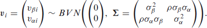
Fitting the model that assumes the bivariate normal distribution for the frailty terms avoids the potentially restrictive assumption of independence. Although we only consider the normal distribution for the random effects here, estimates of the fixed effects
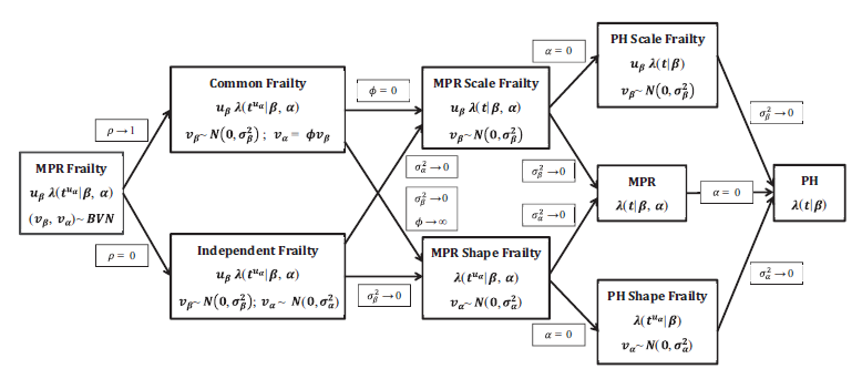
Key sub-models via parameter constraints
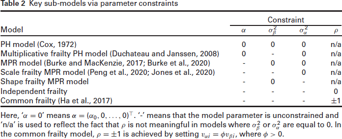
A schematic diagram of some of the possible models generalized by the proposed MPR frailty model. Note: When going from the Common Frailty model to the MPR Shape Frailty model, the interpretation is that
and
but
is a constant;
.
Here, ‘
Denoting the observed data by the pairs 
where

is the logarithm of the conditional joint density function for tij and δij given the random effects 
is the logarithm of the density function of vi with dispersion parameters (i.e., frailty parameters)
From the h-likelihood function given in (2.2), we can derive two likelihoods, namely the marginal likelihood and the restricted likelihood. The marginal likelihood eliminates the random effects,
where
With the exception of binary data with a small cluster size (i.e.,
The h-likelihood function given in (2) is maximized to obtain the maximum h-likelihood estimators (MHLEs) of 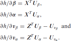
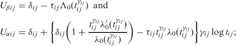
and 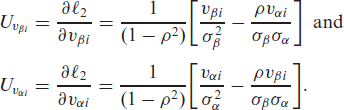
The corresponding observed information matrix can be written explicitly as
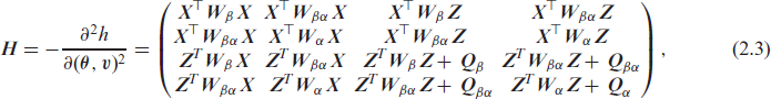
where 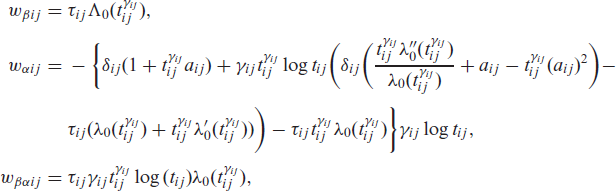
where 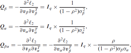
where 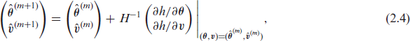
where 
Here,
The model estimation algorithm described above can be summarized as follows:
Using 0.01 as the initial values for the scale and shape coefficients, we fit a fixed effects Weibull MPR model. Estimates from this model are used as the initial values for the fixed parameters,
Step 1 Keeping the frailty variance parameters
Step 2 Given the estimates
Iterate between Step 1 and Step 2 until the convergence criterion is met, that is until the maximum absolute difference between the previous and current estimates for (
From the simulations we have carried out, we have found the algorithm to be computationally efficient, and it has almost always converged except for a small number of cases when the censoring percentage is high and the sample size is small (e.g., 50% censoring under (q, ni). After convergence, the validity of our estimates is confirmed by comparing with the true parameters in the simulation scenario, for example, the estimation bias decreases asymptotically.
Simulation studies
The performance of the proposed methods is evaluated through simulation studies. The Weibull distribution is one of the most commonly used distributions in survival analysis, and hence, we chose to generate the survival times from a Weibull MPR frailty model with the following regression parameters
The corresponding covariates,
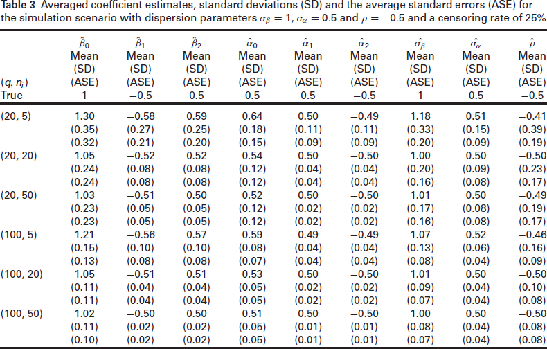
Averaged coefficient estimates, standard deviations (SD) and the average standard errors (ASE) for the simulation scenario with dispersion parameters
and
and a censoring rate of 25%
Averaged coefficient estimates, standard deviations (SD) and the average standard errors (ASE) for the simulation scenario with dispersion parameters
and
and a censoring rate of 25%
Coverage probabilities
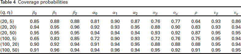
Overall, the h-likelihood estimates of both the fixed parameters and the frailty dispersion parameters perform quite well. The bias in the estimates is reduced as we increase both the cluster size and the number of clusters: this is observed in all the combinations of dispersion parameters and for both censoring percentages considered. The standard errors appear to be underestimated in the smaller sample sizes. This is especially true for the frailty variance parameters, and to a lesser extent, for the fixed effects. As we increase the cluster size and the number of clusters, however, we see that the standard errors reduce for all the parameters, and the ASE converges towards the SD. Similarly, we see from Table 4 that the empirical coverage of the nominal 95% confidence intervals improves with the cluster size, albeit this convergence is slower for the frailty parameters. These findings are in line with the fact that the adjusted profile likelihood
Modelling details
We also illustrate the proposed models on two datasets. Though our main focus is the MPR model with BVN frailties, for the purpose of comparison and analysis, we also consider various simplifications of this model. More precisely, we fit Weibull MPR models with the following frailty structures to each of the datasets we consider.
BVNF: BVN frailty IF: independent frailty CF: common frailty ScF: scale frailty only ShF: shape frailty only
These models are fitted following the procedures described in Sections 2.3 and 2.4, and the standard errors for the estimated parameters are computed as described in Section 2.3. For the selection of the fraily structure that is best supported by the data, we use the Akaike information criterion (AIC). Various extended definitions of the AIC in random-effect models can be formulated based on different likelihood functions (Vaida and Blanchard, 2005; Xu et al., 2009; Ha et al., 2007, 2017). More specifically, we make use of the restricted AIC (rAIC) (Ha et al., 2007) and the conditional AIC (cAIC) (Vaida and Blanchard, 2005; Ha et al., 2017). The rAIC is based on the restricted likelihood approximation 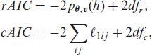
where dfr is the number of dispersion parameters governing the frailty distribution,
In the Weibull MPR models (or any other parametric MPR model with a scale and shape parameter), the scale coefficients describe the overall scale of the hazard and the shape coefficients describe its evolution over time. A positive scale coefficient indicates an increase in the hazard relative to some reference category and similarly, a positive shape coefficient indicates an increasing hazard over time relative to some reference category. While an examination of the 
where
Extensive-stage small-cell lung cancer
This dataset was collected as part of a randomized, multi-centre study conducted by the Eastern Cooperative Oncology Group (ECOG). The main purpose of the trial was to determine if cyclic alternating combination chemotherapy was superior to cyclic standard chemotherapy in patients with extensive-stage small-cell lung cancer. Patients were randomly assigned to one of two treatment arms: standard chemotherapy (CAV; reference category) or an alternating regimen (CAV-HEM). The dataset includes 579 patients from 31 different institutions, with the number of patients per institution ranging from 1 to 56 and a median of 17 patients per institution. The outcome variable was time (in years) from randomization until death. The median survival time and maximum follow-up time were 0.86 years and 8.45 years, respectively, and of the 579 study participants, only 10 were censored yielding a censoring rate of approximately 1.7%. Besides the survival time, censoring status, institution code and treatment, four other dichotomous variables were included in this dataset, namely (reference category listed first): the presence of bone metastases (no, yes), the presence of liver metastases (no, yes), patient status on entry (confined to bed or chair, ambulatory), and whether there was weight loss prior to entry (no, yes). More details on the trial and its clinical results can be found in Ettinger et al. (1990). This dataset was also previously analysed in Gray (1994) using a fully Bayesian approach, in Vaida and Xu (2000) using a marginal likelihood approach, and in Ha et al. (2016b) using a correlated frailty model fitted using a h-likelihood approach.
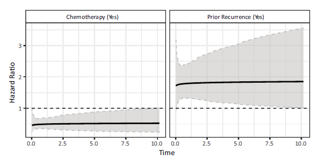
The coefficient estimates, frailty dispersion parameter estimates and estimated standard errors (in brackets) from each model we fit to the lung cancer dataset
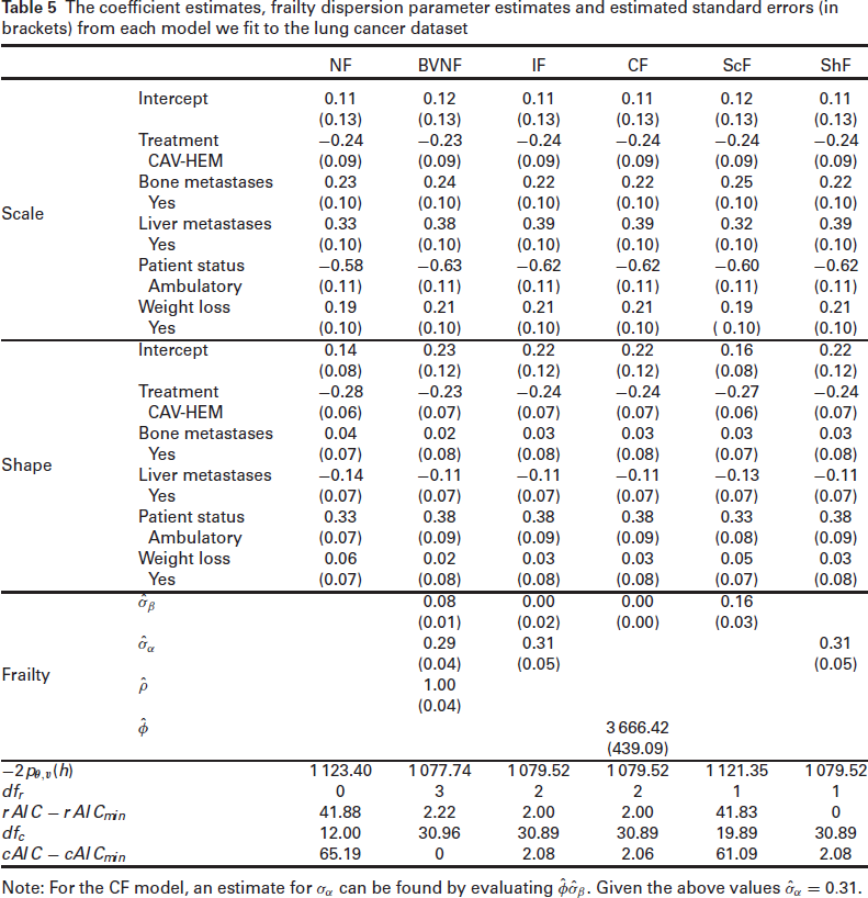
The coefficient estimates, frailty dispersion parameter estimates and estimated standard errors (in brackets) from each model we fit to the lung cancer dataset
Note: For the CF model, an estimate for
With the exception of the ScF model, all the models containing at least one frailty component have quite similar rAIC values, all much smaller than the rAIC value from a no frailty model, with the model with a frailty term in the shape only, the ShF model, having the lowest value. The ScF model, which is the more standard multiplicative frailty model, has a similar rAIC value to the model with no frailty components; this suggests that the baseline risk is homogenous across the centres and a frailty term in the scale is not needed. We observe a similar pattern in the cAIC values, in that all the models containing at least one frailty component (with the exception of the ScF model) have similar cAIC values and all much smaller compared to the NF model. Although the BVNF model has the lowest cAIC value, it is still close to those of the IF, CF, and ShF models. Given this, and also the rAIC values, we consider the ShF as the ‘best’ model.
Although we report the standard errors of the frailty variance parameters, one should not use them for testing the hypothesis
We now focus on the results from the model selected by the rAIC, the ShF model. Considering the scale parameter results first, all the variables included in the model have significant scale coefficients. The CAV-HEM treatment and the subject being ambulatory on entry have negative scale coefficients and so reduce the hazard of death relative to their respective reference categories, the CAV treatment and subject being confined to bed or chair on entry respectively. The presence of bone metastases, the presence of liver metastases and weight loss prior to study entry are all found to increase the hazard of death relative to their reference categories. Now, considering the shape parameter, only two variables, treatment and patient status on entry, have significant coefficients. The CAV-HEM treatment has a negative shape coefficient suggesting that the hazard further decreases over time, relative to the reference category. The positive shape coefficient for the subject being ambulatory on entry suggests that the hazard increases over time. Thus, although this variable has an initial effect of reducing the hazard of death, this effect wears off over time, relative to its reference category.
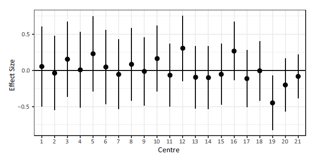
Figure 2 shows the hazard ratio corresponding to each of the variables in our model along with 95% confidence intervals estimated using a parametric bootstrap (Davison and Hinkley, 1997). The presence of bone metastases and weight loss prior to study entry appear to have a more or less constant hazard over time, which is expected since their corresponding shape effects are quite small and not significant. The presence of liver metastases has a negative effect on the hazard but this effect wears off within the first 2 to 3 years. The hazard ratio for the patient being ambulatory on entry appears to be increasing over time. The effectiveness of the CAV-HEM treatment is only observed after 2 months or so from the treatment start date and the hazard continues to decrease over time relative to the CAV treatment.
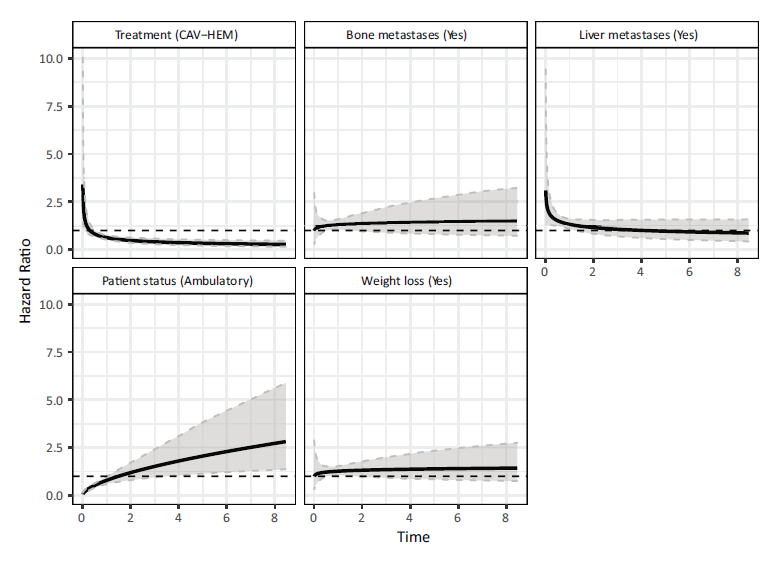
Note: The modal values were used in the computation of these hazard ratios (Treatment = CAV, Bone Metastases = no, Liver Metastases = no, Patient Status = ambulatory on entry, Weight Loss = yes).
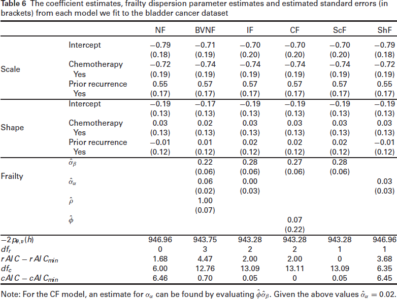
The random effects along with their 95% confidence intervals under the ShF model are shown in Figure 3. Note that as the cluster size increases, the confidence bounds around the cluster effect shrink. The biggest changes in centre specific hazard over time can be seen in centres 12, 16 and 20. A positive frailty suggests the hazard is increasing over time relative to the baseline, while a negative one suggests it is decreasing relative to the baseline.
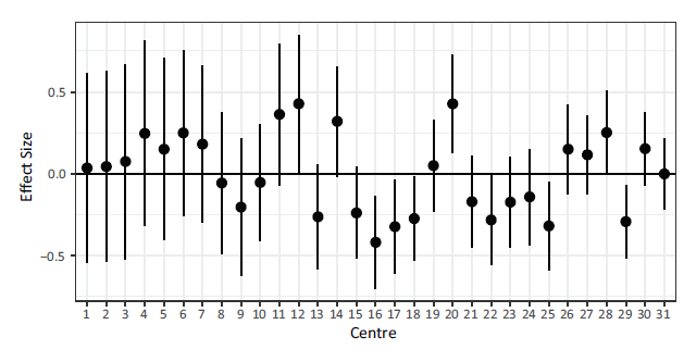
Note: Centres are sorted in increasing order based on the number of patients.
This multi-centre dataset was collected as part of the European Organisation for Research and Treatment of Cancer (EORTC) trial 30791 (Sylvester et al., 2006). A total of 410 patients with superficial bladder cancer were included in this dataset. The patients came from 21 different centres and the number of patients per centre varied between 3 and 78 patients with a median of 15 patients per centre. The outcome variable is relapse-free or disease-free interval after transurethral resection, that is, time from randomization until cancer relapse. Patients who did not experience a recurrence during the follow-up period were censored at their last date of follow-up. The maximum follow-up time was 10.16 years and 204 of the 410 patients (approximately 50% of the patients) were right-censored. The two covariates included in this dataset are (reference categories are listed first): a treatment indicator for chemotherapy (no, yes) and a variable representing the prior recurrence (no, yes). This dataset was also previously analysed in Ha et al. (2011) and can be found in the
The coefficient estimates, frailty dispersion parameter estimates and estimated standard errors (in brackets) from each model we fit to the bladder cancer dataset
The coefficient estimates, frailty dispersion parameter estimates and estimated standard errors (in brackets) from each model we fit to the bladder cancer dataset
Note: For the CF model, an estimate for
Similar to the previous example, the correlation coefficient between the two random effects,
The difference in deviance,
Note: Centres are sorted in increasing order based on the number of patients.
Focusing on the results from the ScF model, both variables included in the model have significant scale coefficients but non-significant shape coefficients. The variable Chemotherapy has a negative coefficient and so the hazard is significantly reduced, that is, time until recurrence is prolonged for patients that received chemotherapy relative to those who did not. Prior recurrence has a positive coefficient and so having had a recurrence already significantly increases the risk of another recurrence, relative to it being a primary occurrence. The shape coefficients corresponding to the two variables, albeit non-significant, are both positive, suggesting that the effect of chemotherapy wears off over time, and also the risk of another recurrence increases with time after a prior recurrence. Plots of the hazard ratios along with their bootstrapped 95% confidence intervals can be seen in Figure 5. As expected, the two variables have approximately constant hazards over time and so perhaps the model can be reduced to a PH model.
Note: The modal values were used in the computation of these hazard ratios (Chemotherapy = yes, Prior Recurrence = no).
The MPR frailty modelling framework we have proposed not only includes frailty structures that have not been previously explored in the literature, but also generalizes a variety of existing sub-models. Existing literature on MPR frailty models has been limited to multiplicative frailty, and, to the best of our knowledge, a model with correlated frailty in each distributional parameter has not previously been considered. We believe that this is a natural structure in the context of MPR modelling, since it has been shown that estimates of the scale and shape can be quite correlated in practice (Burke and MacKenzie, 2017); hence, it is useful to allow for the possibility that correlation may propagate to the frailty terms.
Although the numerical studies were carried out on a Weibull MPR model, we have developed the model and the estimation procedure in a generic form; the underlying cumulative hazard function can be replaced with that of any other two parameter distribution. In principle, the methods can also be extended to models with more than two distributional parameters, for example, the power generalized Weibull model of Burke et al. (2020), using a higher order multivariate normal distribution but this is beyond the scope of this article. The adopted h-likelihood framework provides a computationally inexpensive and straightforward two step procedure to fit our frailty models, avoiding the often intractable integration of the random effects over the frailty distribution. Moreover, the readily available estimates of the frailties allow for the survivor function for individuals with specific characteristics to be estimated, and this is useful in providing information about the merits of the different centres in terms of patient survival in multi-centre studies.
While the proposed MPR framework provides a very flexible approach to modelling correlated survival data at a minimal computational cost, there are various ways in which we can extend it to handle more complicated frailty structures. All of the models that we have considered have a constant frailty variance, perhaps a natural next step for us is to allow the frailty variance to depend on covariates in a similar fashion to that of Peng et al. (2020). Another potential direction worth exploring would be multilevel or nested frailty structures. We can have data on patients, nested within centres or hospitals, with recurrent event times; hence, we may need a frailty component for the patients and a frailty component for the centre or hospital. The procedures we present can be straightforwardly extended to include more than one random component for each distributional parameter.
Supplementary material
Supplementary material is available online.
Supplemental Material for Multi-parameter regression survival modelling with random effects by Fatima-Zahra Jaouimaa, Il Do Ha, Kevin Burke, in Statistical Modelling
Footnotes
Declaration of Conflicting Interests
The authors declared no potential conflicts of interest with respect to the research, authorship and/or publication of this article.
Funding
This work was funded by the Irish Research Council and the National Research Foundation of Korea (NRF) grant funded by the Korea government (MSIT) (No. NRF-2020R1F1A1A01056987). This work was also supported by the Confirm Smart Manufacturing Centre (
References
Supplementary Material
Please find the following supplemental material available below.
For Open Access articles published under a Creative Commons License, all supplemental material carries the same license as the article it is associated with.
For non-Open Access articles published, all supplemental material carries a non-exclusive license, and permission requests for re-use of supplemental material or any part of supplemental material shall be sent directly to the copyright owner as specified in the copyright notice associated with the article.