
Abstract
Prediction models in credit scoring are often formulated using available data on accepted applicants at the loan application stage. The use of this data to estimate probability of default (PD) may lead to bias due to non-random selection from the population of applicants. That is, the PD in the general population of applicants may not be the same with the PD in the subpopulation of the accepted applicants. A prominent model for the reduction of bias in this framework is the sample selection model, but there is no consensus on its utility yet. It is unclear if the bias-variance trade- off of regularization techniques can improve the predictions of PD in non-random sample selection setting. To address this, we propose the use of Lasso and adaptive Lasso for variable selection and optimal predictive accuracy. By appealing to the least square approximation of the likelihood function of sample selection model, we optimize the resulting function subject to L1 and adaptively weighted L1 penalties using an efficient algorithm. We evaluate the performance of the proposed approach and competing alternatives in a simulation study and applied it to the well-known American Express credit card dataset.
Introduction
Credit scoring models are used to evaluate the likelihood of credit applicants defaulting in order to decide whether to grant them credit. The scoring systems are based on the past performance of consumers who are similar to those who will be assessed under the system. In other words, several loan applicant attributes are used to assign a score. These scores are used to determine credit worthiness of the applicant. In practice, the credit scores are transformed into the probability of default (PD). PD is the expected probability that a borrower will default on the debt before its maturity. A key concern in the use of these models is that they are typically designed and calibrated using data from applicants who were previously considered adequately creditworthy to have been granted credit (Banasik et al., 2003). Consider, as an example, where a loan application is made to a bank. The bank uses the loan applicant attributes to grant or reject the loan request. If the request is accepted, then the bank will observe the loan performance over time. Marshall et al. (2010) classified these procedures into two: the credit granting process (accept or reject) and loan performance process (default or non-default). A model developed using the accept-only applicants from the credit granting process may be a non-random sample from the target population and can lead to selection bias.
A strategy for addressing the problem of sample selection bias in credit scoring is the reject inference techniques (Hand & Henley, 1993; Crook & Banasik, 2004). Reject inference is the process of inferring how rejected loan applicants would have behaved had they been granted loan. The techniques for reject inference can be classified under two different assumptions (Kim & Sohn, 2007). The first assumption is that the distribution pattern of accepted applicants can be extended to that of rejected ones. That is, P(default X, rejected) P(default X, accepted), where X is the vector of applicants’ attributes. This implies that PD in the population of accepted applicants can be applied to the rejected ones. Examples of statistical methods in this category include re-weighting and extrapolation methods. The second assumption implies that P(default X, rejected) P(default X, accepted). In this case, the PD in the population at large, P(default X) cannot be approximated by the conditional model based on P(default X, accepted) for an applicant selected at random from the full population. A widely used method under this assumption is the bivariate probit model with sample selection (Dubin & Rivers, 1989).
There are two discordant viewpoints on the utility of sample selection models for reject inference in the literature. Greene (1998) and Greene (2008), for example, analysed the risk of a loan default for credit cardholders using sample selection model, and concluded that the model with adjustment for sample selection bias exhibits better discrimination than the model based on accept-only data. By taking variable selection into account, Marshall et al. (2010) showed that the model without considering sample selection bias can underestimate PD. Other studies that reported higher model performance can be found in Banasik et al. (2003), Banasik and Crook (2007) and Kim & Sohn (2007). On the other hand, Little (1985) and Crook & Banasik (2004) showed that adjusting for selectivity bias may not yield improved predictions when the proportion of rejected applicants is low. In a simulation study, Wu and Hand (2007) also reported the importance of the proportion of accepted or rejected applicants in reject inference. It was shown that even with the normality assumption in place for sample selection model, correction for selection bias may not improve predictions when the proportion of accepted applicants is large. Further examples can be found in Puhani (2000) and Chen and ˚Astebro (2012).
There are various reasons for the discordant viewpoints mentioned above. These include the proportion of rejected applicants, the inclusion of ‘noise’ variables (variables that are not predictive of PD) in both the loan granting and loan performance processes, which may lead to overfitting, and the degree of correlation between the error terms in loan granting and loan performance processes. Indeed, some of these issues have been dealt with to some extent in the literature. Marshall et al. (2010) used bootstrap variable selection to control for the effect of noise variables, but their method was not optimized for predictions like regularization methods. Data mining techniques have been used in reject inference to improve the quality of credit scorecards, but these are yet to be applied to the Heckman-type selection models (see Li et al., 2017 and references therein). The need to harmonize these issues within the Heckman-type selection models for reject inference is the motivation for this article. The contribution of this article is therefore twofold. First, we introduce Lasso (Tibshirani, 1996) and adaptive Lasso (Zou, 2006) penalized Heckman-type bivariate probit model and assess its performance in identifying predictive features of PD in credit scoring. Since the model is made up of two components, each of which may have different variables, features selection is somewhat complex. Thus, our framework appeals to the unified treatment of L1-constrained model selection of Wang and Leng (2007), which is based on least squares approximation (LSA) of the likelihood function. The resulting LSA is then solved subject to L1 and adaptively weighted L1 penalties using the coordinate descent algorithm. Unlike the bootstrap variable selection approach of Marshall et al. (2010), regularization methods have the advantage of simultaneous estimation of parameters and selection of variables. Second, since variable selection provides sparse solution for the true model with true zero coefficients, the predictive performance of the model can be enhanced. We therefore propose a bootstrap internal validation method (Harrell et al., 1996; Ogundimu, 2019) for both the regularized and unregularized sample selection models. Unlike in previous work, where model validation is done using hold-out sample, the bootstrap approach can be used to quantify the degree of optimism in the model. The remainder of the article is organized as follows. In Section 2, we describe the dataset used in the study. The bivariate probit model with sample selection (BPSSM) and its extension using copula-based sample selection model (CBSSM) are described in Section 3. We develop Lasso and adaptive Lasso estimators for the models and provide the computational algorithm for its maximization in Section 4. In Section 5, we describe five metrics for predictive performance that are not threshold dependent and the procedure for internal validation. Simulation study and data example are presented in Section 6. Finally, in Section 7, we provide concluding remarks and further results are presented in Supplementary Materials. We also provide a package in R (HeckmanSelect) for the implementation of the methods.
Dataset
We used the American Express credit card dataset (Greene, 1998, 2008) in this study. The dataset consisted of 13,444 observations on credit card applications received in a single month in 1988. Of the full sample, 10,499 applications were approved, and the next 12 months of spending and default behaviour were observed. Important variables in the data include demographic and socioeconomic factors of the applicants (e.g., Age, Income, whether the applicant owns his or her home, whether the applicant is self-employed or not and the number of dependents living with the applicant). An important factor for granting the credit facility is grouped under ‘Derogatories and Other Credit Data’. These influential variables are number of major and minor derogatory reports (60-day and 30-day delinquencies). Details of the variables used in this study can be found in Table A1 (Supplementary Materials).
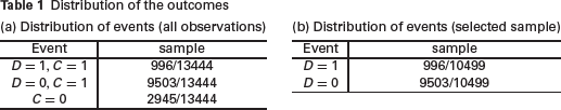
The dataset consisted of two outcome variables–Cardholder status (C), which takes 1 if the application for a credit card was accepted and 0 if not, and Default status (D) which takes 1 if defaulted and 0 if not. Default is defined as having skipped payment for six months, and the corresponding status is observed only when C = 1, that is for 10,499 observations.
Table 1a shows the distribution of the cardholder status. Out of the 13,444 applicants, 2,945 (21.9%) are censored, 996 (7.41%) of those that are selected to receive the card defaulted and 9,503 (70.7%) applicants paid back their loans. Table 1b shows the default status distribution of the selected sample. As it is common in credit scoring, the event rate is less than 10%.
Distribution of the outcomes
Distribution of the outcomes
The use of sample selection model in reject inference assumes that

This implies reject inference can be construed as a missing data problem under the assumption of missing not at random (MNAR) and Heckman selection model can be adapted for parameter estimation and inference. Henceforth, we treat the loan granting process (accept/reject) as the selection equation (Si) and loan performance (default/non-default) as the outcome submodel of interest (Yi).
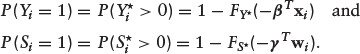
Let Y٨ and S٨ be two latent (unobservable) variables characterizing the outcome and selection equations respectively. That is,
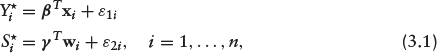
where 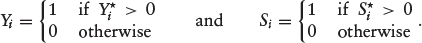
The probability mass function (PMF) of Yi and Si is Bernoulli, where the probability of success depends on the parameters
Suppose that the error terms in equation (3.1) follow a bivariate normal distribution
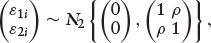
we have the classical bivariate probit model. The selection process is such that Yi is observed if Si = 1, and Yi is missing if Si = 0. There is no selection bias when ρ = 0. In this case, the missing data mechanism is said to be ignorable.
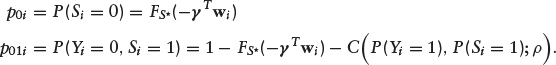
Now, we have three levels of observability: Si = 0 (rejected loans), Si = 1, Yi = 0 (accepted loans and non-default) and Si = 1, Yi = 1 (accepted loans and default). Thus,
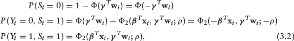
where Ф(·) and Ф2(·, ·; ρ) denote the univariate and bivariate standard normal cumulative distribution functions (CDF) respectively. The appropriate log-likelihood function is easily derived from equation (3.2) as
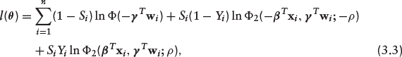
where 
It is straightforward to show that equation (3.4) reduces to Ф(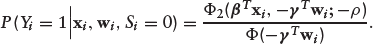
The evaluation of the performance of our method is based on equation (3.4). This is the PD given that a loan is accepted.
Although there is no reason to discountenance the symmetric dependence and the underlying normal assumption used in Section 3.1 for prediction purposes, the model can be generalized using copulas. Let us define the marginal CDFs of Y٨ and S٨ as 
where C(·, ·) is a two-dimensional copula function,
Since the realized ‘outcomes’ Y and S are both binary, we can define the probability of event (Yi = 1, Si = 1) as

where
In addition,
Thus, the likelihood function in equation (3.3) can be generalized as

If we assume a Gaussian copula with normal marginals, that is 
Details of various copulas that can be used in non-Gaussian sample selection models, including the marginal distributions can be found in Marra et al. (2017b) and Gomes et al. (2019). We illustrate the proposed method using Ali–Mikhail–Haq (AMH) copula function with Gaussian marginal distribution for both the outcome and the selection equations. We note that AMH copula can only allow for relatively modest dependence (see Section A.3. in Supplementary Materials), and as such, we only consider comparable dependence between the outcome and the selection process of BPSSM and CBSSM in our simulation settings.
Lasso and adaptive Lasso for BPSSM and CBSSM
Ogundimu (2021) introduced a regularization method for sample selection model for continuous outcomes. We generalize the method to binary outcomes by using the unified Lasso approach of Wang and Leng (2007). Since the model is a two-component model, similar to mixture models, we adapt the method implemented in Zeng et al. (2014).
Consider the log-likelihood function l(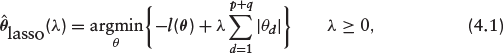
where the second term in the RHS of equation (4.1) is the L1-penalty which shrinks small coefficients to zero to obtain sparse representation of the solution and λ is a tuning parameter controlling the amount of shrinkage, often chosen via cross-validation. The optimization problem reduces to the familiar maximum likelihood estimation when λ = 0.
Equation (4.1) does not have a closed form solution and various algorithms for its computation have been studied. These include the shooting algorithm (Fu, 1998), the least angle regression (LARS; Efron et al., 2004) and the coordinate descent algorithm (Friedman et al., 2007). Since the Lasso penalizes all the regression coefficients equally, it over-penalizes the important variables thereby resulting in biased estimators. The lack of the oracle property (Fan & Li, 2001) of Lasso prompted the development of the adaptive Lasso (Zou, 2006) with this property. The oracle property implies the method is consistent in variable selection, unbiased and asymptotically normal. The estimator is defined as
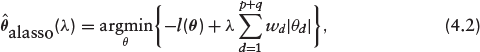
where
It is not straightforward to optimize the penalized log-likelihood function in equation (4.2). To simplify the optimization problem, we approximate l(
where lr(·) and lrr(·) are the first- and second-order derivatives of the log-likelihood function. Since 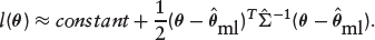
We fitted the models and obtain 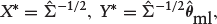
where X∗ is a square matrix containing all the (p + q + 3) predictors along with the correlation parameter ρ and the intercepts, and Y∗ is the corresponding pseudo response. Thus, equation (4.2) can be re-written as
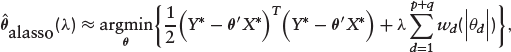
which we optimized using the coordinate descent algorithm (see Friedman et al., 2010; Simon et al., 2011; Ogundimu, 2021).
The optimal tuning parameter, λ can be estimated by using AIC (Akaike information criterion), BIC (Bayesian information criterion) and GCV (generalized cross-validation). It has been shown that the combination of the adaptive Lasso penalty and BIC-type tuning parameter selector results in LSA estimator that can be as efficient as the oracle estimator (Wang et al., 2007). Thus, we focus on the BIC criterion although the method is implemented for both AIC and GCV as well. The expression is given as

where 0 ≤ d fλ ≤ (p + q) is the degree of freedom corresponding to the number of nonzero coefficients of
Variance estimation
The variance of the nonzero component of 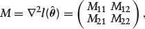
where M11 corresponds to the first r × r submatrix of M. Further, let A11 be the first r × r submatrix of
Then,

We have presented the variance estimation formula for the sake of completeness as the focus of the current work is on predictions. Further details on variance estimation for regularized sample selection model can be found in Ogundimu (2021).
Performance metrics and bootstrap validation
We describe the metrics for predictive accuracy and the bootstrap approach for model validation.
Metrics for predictive performance
In credit risk assessment, the misclassification of loan defaulters into non-defaulters will result in a loss for banks/creditors. Therefore, it is more important that the true defaulters are correctly classified. Here, we focus on model evaluation criteria for predictions in the context of regression analysis rather than classification. This is to ensure that the metrics for predictive performance are not threshold dependent and the users of the model can determine the appropriate threshold for classification. Unlike in previous studies, where area under the curve is the most common metric of prediction accuracy, we examined the performance of four other metrics based on model discrimination and calibration. The following performance metrics are used:
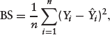
Area under the receiver operating curve (AUROC): The c-index (Harrell et al., 1982) is the generalization of the AUROC, which is a measure of model performance that separates subjects with the event of interest from subjects without the event (discrimination). It calculates the proportion of pairs in which the predicted event probability is higher for the subject with the event of interest than that for the subject without the event. A model with no discriminatory ability has a value around 0.5 whereas a value close to 1 suggests excellent discrimination. Area under the precision-recall curve (AUPRC): Suppose True positive (TP) is defined as actual defaulters who are correctly predicted, False negative (FN) as actual defaulters who are predicted as non-defaulters, and False positive (FP) as actual non-defaulters predicted as defaulters. Then, Recall = TP/(TP + F N) and Precision = TP/(TP + F P). Thus, the precision-recall curve shows the relationship between precision and recall for every possible threshold value. The area under the curve is a single number summary of the information in the precision-recall (PR) curve. A key advantage of AUPRC is that it takes into consideration the prior probability of the outcome of interest, thereby reflecting the ability of the model to identify defaulters (often the minority class in credit scoring). Unlike the AUROC, its values range from 0 to 1. Its value approaches 0 as the prior probability of the outcome decreases (Davis & Goadrich, 2006). We computed this metric by using the PRROC package in R (Grau et al., 2015). Brier score (BS): It is a measure of agreement between the observed binary outcome (i.e., default versus non-default) and the predicted PD as shown below
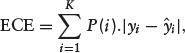
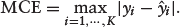
where Yi is the outcome and Calibration Metrics: We consider two metrics of calibration–Expected Calibration Error (ECE) and Maximum Calibration Error (MCE). The metrics are computed by sorting predicted probabilities and partitioning it into K fixed number of equal-frequency bins. The ECE calculates the average calibration error over the bins as
where yi is the true fraction of positive instances in bin i, The choices between K = 10 and K = 100 have been reported in the literature (Naeini et al., 2015; Wang et al., 2019). We chose K = 10 in this study. Like Brier score, the lower the values of ECE and MCE, the better is the calibration of a model.
Bootstrap internal validation
Although we implemented penalized sample selection models to alleviate overfitting, some degree of optimism may persist, nonetheless. Harrell et al. (1996) presented a procedure for estimating optimism in predictive models. We extend this method to incorporate variable selection. Without loss of generality, consider a dataset
Take a bootstrap sample
b
from fit model to
b
using regularized sample selection model (grid search for optimal λ is done on each
b
) predict on the same
b
sample and compute predictive accuracy metric of interest, say use the model to predict on compute average optimism:
fit model to
use the model to predict on
The optimism corrected metric P is the metric that has been corrected for overfitting. It is noteworthy that optimal lambda value is selected for each of the b bootstrap sample.
Numerical studies
In this section, we use simulation and a real data to evaluate the utility of the proposed estimators in reject inference.
Simulation study
We generated 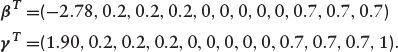
The intercepts of the outcome equation, β0 = -2.78 and the selection equation, γ0 = 1.90 are chosen such that the required event rate and missing data is about 10% and 22% respectively. The 10% event rate is typical of datasets for modelling PD (Ogundimu, 2019). The simulation design ensures that there is one predictor in the selection equation that is not in the outcome equation (exclusion restriction– although this is not essential as demonstrated in Ogundimu, 2021). The covariates
BPSSM: the errors are generated with mean zero and correlation matrix
CBSSM: the errors are generated from AMH copula with association measure θAMH = {0, 0.498, 1}. Note that these values are equivalent to the values of ρ in the distribution of error terms under BPSSM. Specifically,
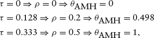
where τ is the Kendall’s tau.
The covariates x1,..., x8 are generated such that their distribution are marginally standard normal with pairwise correlations
We evaluated three classes of models: Bivariate probit model with sample selection (BPSSM), Copula bivariate sample selection model (CBSSM) and accept-only probit model (PROBIT). That is, adaptive Lasso penalized BPSSM (BPSSM ALasso), Lasso penalized BPSSM (BPSSM Lasso) and BPSSM with variables selected using p-value at 5% level of significance (BPSSM P-value). For the copula-based model, we have adaptive Lasso penalized CBSSM (CBSSM ALasso) and Lasso penalized CBSSM (CBSSM Lasso), while the accept-only model includes probit model with adaptive Lasso (PROBIT ALasso), probit model with Lasso (PROBIT Lasso) and probit model with p-value (PROBIT P-value).
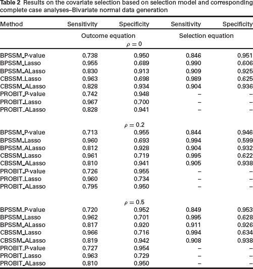
We evaluated the performance of the methods using sensitivity (mean of proportion of nonzero coefficients that were correctly identified) and specificity (mean of proportion of zero coefficients that were correctly identified). The predictive accuracy of the model is evaluated using bootstrap method as described in Section 5. For each bootstrap sample, optimal λ is computed over a grid of candidate values of λ as described in Section 4.3 to provide a model having predictors and coefficients based on that penalty.
In Table 2, we present the results of the sensitivity and specificity of the methods for variable selection. Lasso methods have higher sensitivity but lower specificity than the other methods. This observation is not surprising since Lasso estimator lacks oracle property (Zou, 2006) and it is generally known to include true covariates, but also irrelevant covariates (Meinshausen & Bu¨ hlmann, 2006). Although the data was generated based on a bivariate normal distribution, the performance of CBSSM methods is superior to the corresponding BPSSM methods in terms of specificity. There is no clear distinction among the methods in terms of sensitivity. The adaptive Lasso methods have slightly better overall performance on the combined effects of sensitivity and specificity. To see the impact of weak and moderate covariate effects on the methods, we present the frequency with which the variables are selected in 200 replications in Table 3. The unregularized methods (BPSSM_P-value and Probit_P-value) selected true covariates less often when the effect is weak, but it is slightly better in selecting fewest covariates with true zero coefficients. CB-SSM_Lasso is slightly better than BPSSM_Lasso across the correlation values. There is no clear advantage of sample selection models over complete case analyses in Tables 2 and 3.
Results on the covariate selection based on selection model and corresponding complete case analyses–Bivariate normal data generation
Results on the covariate selection based on selection model and corresponding complete case analyses–Bivariate normal data generation
Simulation results for the number of times each covariate is selected (out of 200) with both weak and moderate covariate effects (Outcome equation)–Bivariate normal data generation
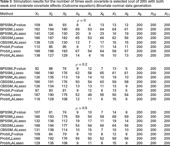
Table 4 shows the result of quantifying optimistic predictions in the models. Regularized methods are expected to exhibit smaller optimism as the regularization is meant to alleviate the problem of overfitting. The results indicate that the use of sample selection models in reject inference problem, whether regularized or not, does not improve the accuracy of complete case analysis. Lasso-based methods are slightly better than the other methods in terms of the metrics for discrimination (AUROC and AUPRC). This is counterbalanced by its performance on the two metrics for calibration (ECE and MCE), where calibration results are consistently poorer than the other methods. This may be due to the inclusion of unimportant variables in Lasso methods.
Results of the optimism corrected model performance–Bivariate normal data generation
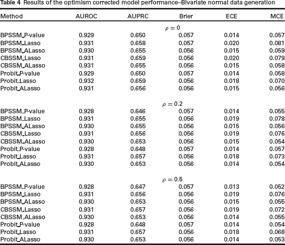
Table A2 in the Supplementary Materials is equivalent to the results in Table 2 but with the data generated from AMH copula. Overall, CBSSM performance is slightly better than BPSSM (due to its performance on specificity). In general, complete case analyses are slightly better in terms of specificity for the outcome model whereas the regularized CBSSM sample selection models are better in terms of sensitivity. CBSSM ALasso is better than BPSSM ALasso (see Table A3 in Supplementary Materials). The results also show that there is slight benefit of the sample selection models over the corresponding complete case analyses. However, the use of sample selection model does not translate to improved predictions (see Table A4 in Supplementary Materials).
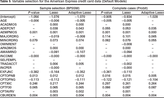
We used the American Express credit card dataset that was described in Section 2 to evaluate the performance of our models. Table 5 gives the variables selected and parameter estimates of the bivariate probit model with sample selection (BPSSM) and classical probit model (PROBIT) for the default equation. The performance of BPSSM Lasso and BPSSM ALasso are similar in terms of the variables that are associated with PD except for the variable INCPER (income per family member), which is retained in the former but not the latter. BPSSM P-value removed 10 variables from the default model, BPSSM ALasso removed three variables and BPSSM Lasso removed two variables. The variables OWNRENT and SELFEMPL are the two variables that are removed from the three models. The models under the complete case analyses (default model only) are based on variable selection using probit regression. Unlike in BPSSM models, PROBIT ALasso shrinks more parameters (10 variables) to zero than PROBIT P-value (eight variables). PROBIT ALasso set AGE and EXP INC to zero whereas these variables are associated with PD in PROBIT P-value method. The only variable set to zero by PROBIT Lasso is SELFEMPL.
Variable selection for the American Express credit card data (Default Models)
Variable selection for the American Express credit card data (Default Models)
The comparison across Table 5 of BPSSM and PROBIT methods show that INCOME, MINORDRG, AEMPMOS, CBURDEN, CPTOPNB, CPTOPNG, CPT30C and CPTF30 are important predictors of PD. The lower the income the more likely for an applicant to default while the higher the credit burden the more likely for the applicant to default. A striking observation is the setting of MAJORDRG to zero in BPSSM P-value model whereas the variable is retained in other models across Table 5. However, all the methods (both under BPSSM and PROBIT) show that MINORDRG is associated with PD.
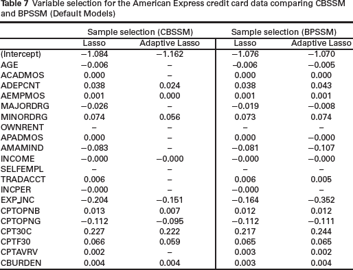
Table 6 shows the results of variable selection in the selection equation of BPSSM models. The performance of BPSSM Lasso and BPSSM ALasso are again similar in terms of the variables that are set to zero except for two variables–AGE and INCPER. Variables OWNRENT and BANKCH are not predictive of selection into the sample. We also fitted the copula model (CBSSM) to the data. Table 7 shows the comparison of the models with BPMSS for the default model. The performance of Lasso methods is similar but coefficients from BPMSS Lasso are shrunk more towards zero than CBSSM Lasso. CBSSM ALasso set 10 variables to zero whereas BPSSM ALasso set only three variables to zero. Again, Lasso models for the cardholder equation are similar (Table 8).
Variable selection for the American Express credit card data based on BPSSM (Cardholder Models)
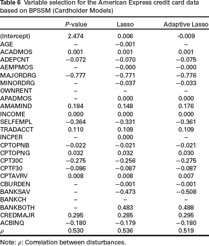
Note: ρ: Correlation between disturbances.
Variable selection for the American Express credit card data comparing CBSSM and BPSSM (Default Models)
Variable selection for the American Express credit card data comparing CBSSM and BPSSM (Cardholder Models)
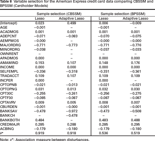
Note: θ∗: Association measure between disturbances.
Tables 9 and 10 show the predictive performance of the methods. There are still some amounts of optimism in the regularized methods. Interestingly, sample selection models are generally superior to complete case analyses in terms of discrimination (except for BPSSM_P-value)- a result that is not definitive from the simulation study.
Apparent model performance in predicting default probability in American Express credit card data
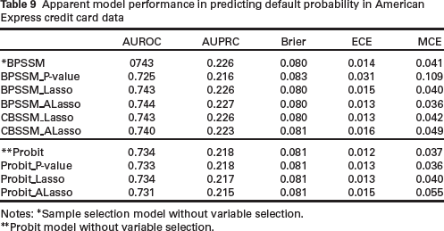
Notes: ∗Sample selection model without variable selection.
∗∗Probit model without variable selection.
Optimism corrected model performance in predicting default probability in American Express credit card data
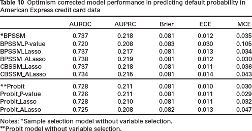
Notes: ∗Sample selection model without variable selection.
∗∗Probit model without variable selection.
In this article, we introduced a variable selection technique based on lasso-type penalty for bivariate binary sample selection model. We also proposed a bootstrap internal validation method for this model. The sample selection models are analysed alongside complete case analyses (accept-only models). The simulation setting was structured to mimic typical rate of event and degree of missing data in practical data (10% event rate and 22% missing information). The results indicated that the proposed regularized sample selection model is suitable for variable selection in credit scoring research. We also concluded that the regularized results based on adaptive Lasso have better combined effects on sensitivity and specificity than the use of p-value, which is threshold dependent. This was the case in both the sample selection and the accept-only models. The simulation results for the internal validation of the prediction models did not provide definitive advantage of using sample selection model over the accept-only model. The cases where the metrics for discrimination are slightly better for the accept-only model were counterbalanced by the sample selection models doing relatively better on metrics for calibration. Overall, our results indicated that Lasso methods should be preferred for optimal predictions.
We have used the AMH copula function with Gaussian marginal distributions in this article. In application, we can incorporate the method of choosing a suitable copula and link function within the proposed framework. One way to do this is by optimizing optimism corrected predictive accuracy measure of interest (e.g., AUROC) over a suitable set of copulas and link functions with relatively small bootstrap samples (say, 20 to 30). What is needed in the current implementation is to add appropriate likelihood function for the copula and link function. The methods in this article are implemented in the R package HeckmanSelect, the package contains a simulated data (binHeckman) and the American Express credit card data (AmEX). It can be installed as follows:
We have used a simulation study with event rate and degree of selection that is similar to the American Express credit card dataset. It is unlikely that varying these factors will change our conclusions significantly. There are limitations of this study that deserved thorough attention. We have used a single penalty term with one tuning parameter for both the outcome and the selection equations, which is quite restrictive. Separate penalties can be used via approximation of the L1 norm. Apart from Lasso and adaptive Lasso, the use of correlation-based penalty, like the one proposed in Tutz and Ulbricht (2009), can alleviate the problem of multicollinearity. There are methods to incorporate more flexible covariate effect structures in sample selection models (e.g., splines and fractional polynomials). The method that we proposed can be readily extended to accommodate this flexibility by combining
LSA framework with group Lasso (Yuan & Lin, 2006). In this case, the flexible parameterization of covariates implies that the selection of one variable in a group will results in the selection of all other variables in the same group. Alternatively, the group bridge estimator (Huang et al., 2009) can be used, where simultaneous selection at both the group and within-group individual variable levels is possible.
Footnotes
Supplementary materials
Supplementary materials for this article are available at
Acknowledgements
The author thanks the editor, associate editor and the referees for their helpful comments which improved the article. The author is grateful to Professor William Greene for the helpful discussion on the conventional assumption of normality for the error terms in the classical binary sample selection model.
Declaration of Conflicting Interests
The author declared no potential conflicts of interest with respect to the research, authorship and/or publication of this article.
Funding
The author received no financial support for the research, authorship and/or publication of this article.