Sage Journals: Discover world-class research

Abstract

We propose a model of retail demand for air travel and ticket price elasticity at the daily booking and individual flight level. Daily bookings are modelled as a non-homogeneous Poisson process with respect to the time to departure. The booking intensity is a function of booking and flight level covariates, including non-linear effects modelled semi-parametrically using penalized splines. Customer heterogeneity is incorporated using a finite mixture model, where the latent segments have covariate-dependent probabilities. We fit the model to a unique dataset of over one million daily counts of bookings for 9 602 scheduled flights on a short-haul route over two years. A control variate approach with a strong instrument corrects for a substantial level of price endogeneity. A rich latent segmentation is uncovered, along with strong covariate effects. The calibrated model can be used to quantify demand and price elasticity for different flights booked on different days prior to departure and is a step towards continuous pricing; something that is a major objective of airlines. As our model is interpretable, forecasts can be created under different scenarios. For instance, while our model is calibrated on data collected prior to COVID-19, many of the empirical insights are likely to remain valid as air travel recovers in the post-COVID-19 period.

Keywords

flight price elasticity mixed non-homogeneous Poisson model P-splines price endogeneity

1 Introduction and literature review

The International Air Transport Association (IATA) estimates that in 2019 there were over 4.54 billion passengers on scheduled flights worldwide, generating revenues of $838 billion dollars (IATA, a). However, profits in the airline industry were notoriously low, even before the advent of COVID-19. For example, the industry average net margin was only 3.1% in 2019 (IATA, a). This forces airlines to seek ever greater competitiveness, including the development of improved revenue management methodologies (Talluri and van Ryzin, 2005). Increasing the accuracy of short-term forecasts of passenger demand, along with estimates of its price elasticity, is one such operational efficiency. In particular, the availability of complete booking databases opens up the possibility of computing both demand forecasts and price elasticities for each individual flight and cabin class in real time. Yet there is surprisingly little work in the statistical or econometric literatures on the modelling of passenger demand at such a disaggregate level—in part because the databases required are large, complex and proprietary. In this article, we do so using a novel flexible statistical model, which we apply to a new and unique dataset of 1 333 712 daily counts of retail bookings for flights on a busy short-haul route. This approach allows us to compute the price elasticity of demand for this route at a daily and flight level resolution.

The data is sourced from the booking and flight databases of a large Western airline and are a complete and accurate record of bookings. Therefore, our data are free from the complex biases that can occur in booking datasets constructed using web crawlers or surveys. The airline wishes to remain anonymous, so throughout this article we refer to it as ‘AirABC’, and do not identify the origin and destination cities of the route. Only AirABC services this route, with alternatives restricted to other modes of transport or indirect flights, so that it is reasonable to consider these bookings in isolation of those for other airlines. Thus, our data are similar to those obtained from a controlled experiment. Tickets for different cabin classes (i.e., economy or business) and route directions are effectively separate products, and in our empirical work we consider bookings in one direction (so-called half-return journey) for the main economy class cabin; although the model can be employed directly for other cabin classes or return journeys.

We model the booking process for each flight as an non-homogeneous Poisson process with respect to the (decreasing) number of days to departure. The booking intensity has both a baseline component and a ticket price adjustment. The baseline component is modelled as additive in covariates, including smooth unknown functions of the flight departure time and day to departure. The price adjustments follow a finite mixture modelled using a multinomial logistic regression (MNL) with probabilities that are additive in covariates, including smooth unknown functions of the flight departure time and day to departure. Such a model is similar to the ‘mixtureof-experts’ models that are popular in the machine learning literature (Jordan and Jacobs, 1994), where each mixture component is called an ‘expert’.

The unknown smooth functions in the baseline intensity and mixture probabilities are modelled semi-parametrically with penalized splines (Wood, 2017, chap. 5). This is important because prior research (Wen and Chen, 2017) and our empirical analysis suggests the effects of the key covariates ‘flight departure time’ and ‘time to departure’ can be highly non-linear. A quadratic penalty is used to ensure smoothness of each penalized spline, with the smoothing parameter selected by minimizing the BIC as in Ruppert et al. (2003) and Kauermann et al. (2009). The inclusion of covariates in this way means that each expert is a semi-parametric Poisson regression and the MNL is also semi-parametric.

From a marketing perspective, the model provides a latent segmentation that accounts for customer heterogeneity (Wedel and Kamakura, 2012) at the daily booking count and flight level. Teichert et al. (2008) highlight the importance of identifying different segments to account for customer heterogeneity in airline passenger demand.

They found more than two latent segments, which is consistent with our empirical work where we find up to seven segments. From a revenue management perspective, because the probability of latent class membership varies at the booking day and flight level, so does the ticket price elasticity. This is a key input into variable pricing frameworks. From a regulatory perspective, segmentation at the daily booking and flight level, as opposed to the customer level, avoids the need to collect individual level data. This is an advantage because the collection of such information can either be a concern to breach data privacy provisions, such as the EU General Data Protection Legislation, or is not available to practitioners. In particular data containing socio-economic and trip characteristics of air travellers as revealed by a preference survey (Wen and Chen, 2017; Teichert et al., 2008) is generally unavailable to the airline, nor can it be used by today’s revenue management systems (Hetrakul and Cirillo, 2014).

A central problem in the estimation of price elasticity using realized demand is that price is likely to be endogenous (Petrin and Train, 2010; Li et al., 2014). We address this using a control function approach similar to that suggested by Marra and Radice (2011) for generalized linear models. We employ the ‘bid-price’ (Talluri and van Ryzin, 2004, p. 31) as an instrumental variable, which is an airline industry displacement measure that varies at both the flight and daily levels. We find strong evidence of all aspects of our proposed model—non-linear covariate effects, customer heterogeneity and price endogeneity—in our empirical analysis of passenger demand. A detailed overview of prior studies of retail demand for passenger flights in the revenue management literature that have features closest to ours is given in Section 1 of the Web Appendix.

Deep models from machine learning are also increasingly used to forecast complex time series with non-linear serial dependencies (Diaconescu, 2008), including in transportation; see Ke et al. (2017), Lin et al. (2018) and Xu et al. (2018) for recent examples. Our proposed nonhomogenous Poisson model has the advantage of being interpretable and provides insights into customers’ behaviour that can be used in different scenarios. We mention this point explicitly since the airline industry market is experiencing dramatic changes through the COVID-19 pandemic (see, e.g., Peterson and Thankom (2020) or IATA (b)). Even though the analysis in this article uses data from prior to the pandemic, many of the empirical insights obtained in the nature and form of the key drivers of demand and price elasticity, as well latent segmentation, are likely to remain valid when air travel recovers post-COVID-19. It also has the potential to provide forecasts under different scenarios. For example, baseline intensity can be adjusted to account for new realities in future passenger demand, while retaining the remaining aspects of the calibrated model, to produce flight-level daily demand forecasts.

To account for any unexplained intraday dependence between bookings for different flights we fit a multivariate model using a Gaussian copula and marginals given by the Poisson model. Dependence may exist between bookings for flights that depart at different times on the same day, because some customers might consider them as substitutes (i.e., when the time of flight is not a significant factor for a passenger). To date, only very few articles analyse the substitution patterns between flights in detail.

One study to do so is Escobari (2017) who analyses passenger choice behaviour using a random coefficient logit model. However, this author found little evidence of significant cross-price elasticity at the departure time level, indicating limited substitution patterns between flights. In line with these results, estimates of the Gaussian copula model using our data suggest only low levels of dependence between bookings on different flights departing on the same day. Full details on the copula model and its application are given in Section 4 of the Web Appendix.

Last, we summarize here our main empirical findings. Correcting for price endogeneity in a mixture model framework has a substantial effect on the estimates of price elasticity, which is underestimated if the price is incorrectly treated as exogenous. Even though the consideration of price endogeneity is not novel to the literature, it is novel in a mixture model framework for latent segmentation. We identify a rich segmentation, with between five and seven latent classes for flights that depart on weekdays, but only two for weekend flights; although there is always at least one price-insensitive and one highly price-sensitive segment. The (a) day of the week on which bookings are made, (b) number of days before departure and (c) time of the day at which the flight departs are all strong non-linear predictors of both the mixture component probabilities and baseline booking intensity. These three covariates all vary by flight and booking day, so that both the demand and price elasticity estimates from the model also vary by flight and booking day. Price-sensitive customers tend to dominate up to 75 days before departure and are replaced by price-insensitive customers closer to the departure date. Interestingly, price elasticities are higher for customers who book on the weekend, compared to those who book their flights on a weekday. Thus, the date of booking (both the day type and the number of days before departure) reveals a great deal about the price elasticity of customers. Similarly, the time of departure of the flight itself is highly revealing, with morning and evening peak time flights having a higher proportion of price-insensitive customers; presumably, because these flights are dominated by customers flying for business purposes. As all of the covariates used in our model are observable, our approach does not depend upon individual customer-level data which is difficult to retain under data privacy provisions, such as the EU General Data Protection Regulation (GDPR). Hence, our segmentation model allows for ready forecasting of elasticity and demand for use in airlines’ revenue management systems and therefore aid AirABC in effective variable pricing by flight and day of booking—an approach that it has adopted in practice.

The rest of the article is organized as follows. Section 2 introduces the new dataset we employ, while Section 3 outlines the flexible Poisson model. The latter includes the mixture model, penalized spline smoothing, penalized maximum likelihood estimation and the approach to endogeniety correction. Section 4 contains the empirical analysis and Section 5 concludes our work. Extensive additional material is provided in the Web Appendix which can be found under www.statmod.org/smij/archive.html. This includes an in-depth literature review, additional empirical results, implementation details and specification of the multivariate Gaussian copula model to account for additional dependence between bookings for different flights.

2 Data

2.1 Setting

The data are extracted from the booking system of AirABC, which provides a complete record of bookings. We analyse flight and matching retail booking data for a busy short-haul route over the two-year period between 1 April 2012 and 31 March 2014. The route is direct between two Western cities, which we do not name to ensure anonymity of AirABC, and for simplicity we only consider flights in one direction. Analysis of demand for this route is of particular interest because during this period only AirABC offered direct flights between these destinations, so that alternatives were limited either to indirect flights and other transportation modes. Both economy and business cabin classes were available, although our empirical analysis focuses on the economy cabin, which is the much larger of the two.

2.2 Flight data

The route has up to 17 flights per day, and from these we exclude flights departing on public or school holidays, or correspond to major fairs, exhibitions and conferences at either the origin or destination cities. For these special day types, it is advisable to build separate models for passenger demand, which differs greatly from that on other departure days. If a flight is cancelled, then we retain all bookings over the days prior to cancellation and do not consider any booking days afterwards. If a flight is rescheduled, we retain the original data on bookings prior to the date of reschedule and consider the initial flight cancelled afterwards. We then create a second flight with the departure details of the rescheduled flight, but with bookings possible only on days after the date of reschedule. With these exclusions and rules, our data includes a total of 9 602 flights scheduled to depart on a total of 730 days.

Flights are scheduled to depart every day of the week. There are also 61 distinct scheduled departure times recorded in our data, with the earliest departure at 06:00 and the latest at 21:55. The variable DDAY records the day of the week (Monday through Sunday) on which the flight departs, and the variable DTIME records the time of the day of the departure; both have a substantial impact on passenger demand.

2.3 Retail booking data

We only consider retail demand, based on bookings made within the published fare structure. Bookings made outside this fare structure, which includes those based on frequent flyer miles, corporate and private tariffs, or by airline staff, are omitted. Moreover, we only consider bookings that were also ticketed. This includes online transactions, where booking and ticketing are completed together. However, it excludes some bookings made by phone or via travel agents, where a booking can be made but is not ultimately ticketed due to non-payment. In addition, as discussed above, if a flight is rescheduled or cancelled by the airline, we retain the bookings in our data. We also retain a booking if the passenger cancels after ticketing, as this usually involves some monetary cost to the passenger.

Both return and single tickets are sold for this route. Purchasing the return ticket is always cheaper than two single tickets for the same two flights. Therefore, the motivation for purchasing each ticket type is likely to be different, so that we separate them. In our empirical work we only consider bookings made as part of a return ticket, both when the flight is the inbound or outbound section of a return ticket. We note that return tickets are more common than single ticket bookings for this route, at 93.1% of total bookings.

We construct booking specific variables as follows. We record the day of the week on which each booking was made (BDAY), along with the number of days prior to departure of the flight (t) and also the price paid (PRICE). Over 96.4% of total economy cabin class bookings were made within 120 days before the departure, and we only consider these bookings in our analysis. Bookings made on the day of departure have a value of t = 0, so that 0 ≤ t ≤ 120. If all flights were open for booking during the 121 day period, there would be a total of 121 9 602 = 1 161 842 possible booking days. However, with flight cancellations and rescheduling as discussed above, the number of booking days in our data is slightly less at 1 109 559.

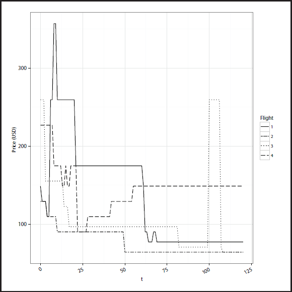
For historical reasons, airlines typically associate each ticket sold with a unique ‘booking class’, which should not be confused with the cabin class (i.e., economy or business). In our data, there are 14 such booking classes which are ordered in terms of increasing price. During the two-year period AirABC changed the fares associated with each booking class only once, which corresponded to an overall price increase. However, on any given day prior to departure, to change the price for a flight the airline simply opens or closes booking classes. This creates substantial variation in fares for each flight during the booking period. The majority of ticket purchases (94%) are at the lowest cost open booking class. The remaining purchases are made at higher cost open booking classes and are termed an ‘upsell’ by AirABC. In our data upsell, bookings do not attract any meaningful additional customer benefits and are likely due to complexities in the booking system. For simplicity, we exclude the small number of upsell bookings from our data, but note that our model can be readily applied to these bookings separately. Overall, there are 442 991 economy bookings recorded in our data for the 9 602 flights. To illustrate the level of variation in ticket prices for a flight, Figure 1 plots the prices (PRICE) of bookings for four typical flights over the 121-day booking period. Prices are quoted in US dollars, although to help ensure anonymity of AirABC, we note that the tickets may, or may not, have been sold in this currency. The four flights were neither cancelled nor rescheduled during the 121-day booking period and all depart at 07:00, which is during the daily peak period. The four price pathways reveal substantial price variation over the booking period, and also across the three flights. This price variation is created by the process of opening and closing booking classes, as discussed above.

Figure 1

Prices of standard bookings (PRICE) for four flights against the time to departure (t), during the 120-day booking window. All three flights were open for booking throughout this window and were scheduled to depart at 07:00

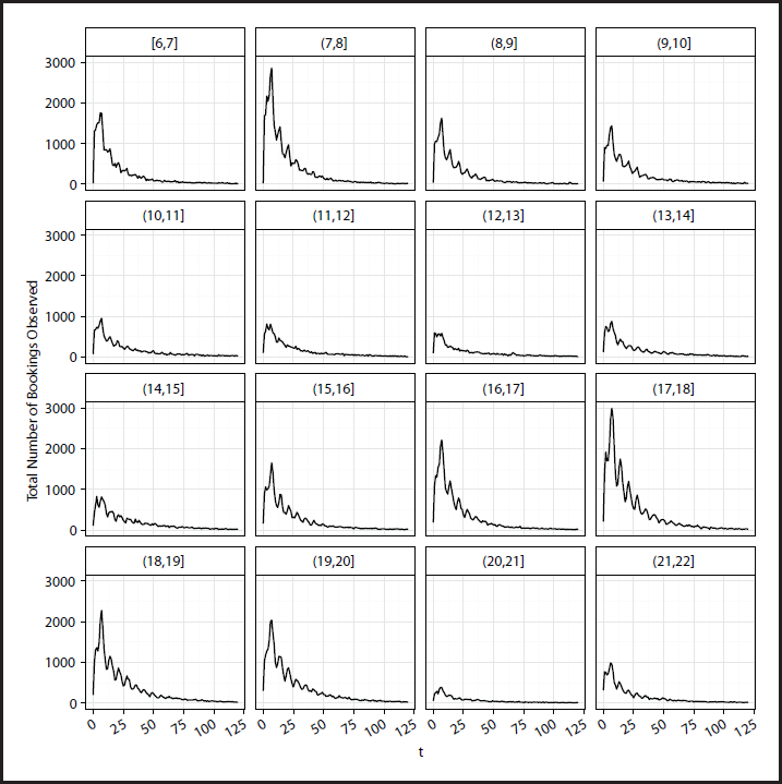
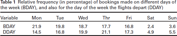
Figure 2 gives the total number of bookings in our data that were made in each seven day interval (i.e., week) prior to flight departure. The bookings are further broken down according to flight departure time, with each panel corresponding to flights leaving during different hourly intervals. Bookings are most heavily concentrated for flights departing between 06:00 and 08:00 and between 17:00 and 20:00. These are morning and evening travel peaks, and are typical of return ticket bookings for a short-haul flight. Regardless of the time of departure of a flight, booking intensity is strongest in the weeks immediately prior to departure; a feature that is again consistent with the short-haul nature of the flight. Last, we note that the day of the week on which the booking was made (BDAY) follows a different distribution than the day of the week on which flights depart (DDAY). To illustrate this, Table 1 provides the relative frequencies of both variables, from which we make three observations. First, bookings are almost exclusively made on weekdays for this route, with around 95% of bookings made between Monday and Friday. Second, while Monday and Tuesday are the most popular days on which to make a booking, Wednesday and Thursday are the most common departure days. Third, only 10% of bookings are for flights that depart on the weekend.

Figure 2

Total number of bookings in our data observed at each day prior to departure date. The bookings are further broken down into hourly intervals of flight departure times, with one panel for each hourly interval. For example, the top left-hand panel plots total bookings made up to 18 weeks prior to departure, only for flights departing between 06:00 and 07:00 (inclusive)

Table 1

Relative frequency (in percentage) of bookings made on different days of the week (BDAY), and also for the day of the week the flights depart (DDAY)

Variable	Mon	Tue	Wed	Thr	Fri	Sat	Sun
BDAY	21.9	19.8	18.7	17.7	16.8	2.4	3.6
DDAY	14.5	16.8	19.9	21.1	17.3	4.9	5.5

3 Model development

3.1 Semiparametric mixed poisson regression for bookings

Let N_i (t) denote the total number of bookings for flight i at t days to departure, which is increasing for t decreasing, so that Y_i (t) = N_i (t) - N_i (t + 1) is the number of passengers who book flight i during day t. Flights departing on each day of the week are considered separately as different products, and DDAY is not incorporated into the notation to aid readability. Because we only consider bookings made up to 120 days prior to departure, we assume N_i (121) = 0, so that N_i (0) is the total number of bookings for flight i made during the 121 day window. The booking process N_i (t) is modelled as a (time-reversed) non-homogeneous Poisson process with intensity λ_i (t) > 0, which is factorized as

λ_{i} (t) = λ_{BL} (t) (\sum_{k = 1}^{K} π_{k} (t) δ_{k})

(3.1)

Here, λ_BL (t) > 0 is a time-varying baseline intensity, while the terms δ₁, …, δ_K are positive adjustments. These adjustments follow a latent finite mixture model with probabilities π₁(t),…, π_K (t), such that 0 ≤ π_k(t) ≤ 1 and $\sum_{k = 1}^{K} π_{k} (t) = 1$ .

Equation (3.1) specifies a non-homogeneous mixed Poisson model for booking activity (Karlis and Xekalaki, 2005), where the intensity follows a discrete mixing distribution with atoms at the points {λ_BL (t)δ₁, …, λ_BL (t)δ_K. The adoption of a mixture model is motivated by previous research which finds latent customer segments based on differing trip purposes and demographics of travellers; for example, see Teichert et al. (2008) and Wen and Lai (2010). To identify these segments, we assume the intensity adjustment δ_k does not vary directly with day to departure, but we allow the probabilities π₁(t), …, π_K(t) to do so instead. However, the baseline intensity, adjustment values and associated probabilities are all functions of further flight and booking level covariates, as now discussed.

Table 1 illustrates that the booking intensity varies greatly with booking day (BDAY), while Figure 2 shows that it also varies substantially with departure time (DTIME) and day to departure (t). The logarithm of the baseline booking intensity is therefore modelled as an additive function of these variables, with

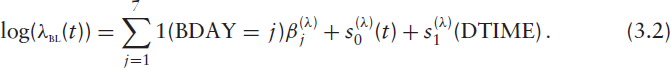
\log (λ_{BL} (t)) = \sum_{j = 1}^{7} 1 (BDAY = j) β_{j}^{(λ)} + s_{0}^{(λ)} (t) + s_{1}^{(λ)} (DTIME)

(3.2)

The term 1(A) is an indicator function equal to one if A is true, and zero otherwise, so that $β^{(λ)} = (β_{1}^{(λ)}, \dots, β_{7}^{(λ)})$ is a vector of booking day intensity effects. Here, the superscript λ distinguishes these baseline booking intensity effects from those for the segment probabilities π_k(t) introduced later. The impact of t and DTIME are modelled as unknown smooth functions $s_{0}^{(λ)}$ and $s_{1}^{(λ)}$ as discussed further below. To identify the level in Equation (3.2), we follow Hastie and Tibshirani (1990) and set the integrals of these functions to zero over their domain.

Previous research (Hetrakul and Cirillo, 2014; Li et al., 2014; Vulcano et al., 2010) indicates there is strong customer heterogeneity in the price elasticity for passenger flights. Our objective in adopting the mixture model is to capture segment specific price elasticities parsimoniously. These are log-linear within each segment, with

\log (δ_{k}) = α_{k} PRICE

(3.3)

The overall price elasticity is therefore $E_{λ} = \sum_{k = 1}^{K} π_{k} (t) α_{k}$ which varies with t and other covariates through the probabilities π(t),…,π_K(t). For modelling these segment probabilities a multinomial logistic regression MNL model is adopted. If segment K is taken as reference category, then the log-odds are

\log (\frac{π_{k} (t)}{π_{K} (t)}) = β_{j, 1} + \sum_{j = 2}^{7} 1 (BDAY = j) β_{j, k}^{(π)} + s_{0, k}^{(π)} (t) + s_{1, k}^{(π)} (DTIME),

(3.4)

for segments k = 1, …, K - 1. This is a semiparametric specification, because the effect of t and DTIME are given by unknown smooth functions $s_{0, k}^{(π)}$ and $s_{1, k}^{(π)}$ . As with the baseline intensity, the functions are constrained to integrate to zero to identify the level in Equation (3.4). The coefficients $β_{k}^{(π)} = (β_{1, k}^{(π)}, \dots, β_{7, k}^{(π)})$ capture the booking day type level effect for segment k, relative to the reference category.

3.2 Penalized likelihood estimation and inference

The unknown functions $s_{0}^{(λ)}, s_{1}^{(λ)}$ for the intensity, and $\{s_{0, k}^{(π)}, s_{1, k}^{(π)}; j = 1, \dots, K - 1\}$ for the MNL model, are modelled using penalized splines. This is a popular approach to smooth function estimation; see Wood (2017) and Ruppert et al. (2009) for overviews and Smith and Kauermann (2011) for their use in transportation science. The advantage of using splines instead of flexible functional forms based on Fourier terms as in Wen and Chen (2017) and Lurkin et al. (2017), is that they allow for data-driven levels of smoothing (i.e., regularization). A penalized spline approximates an unknown function by the inner product of a vector of basis terms w (.) with a coefficient vector γ , so that each function is s(.) w (.)^r γ . Smoothness is achieved by adopting a regularization penalty on γ . For univariate functions, Eilers and Marx (1996) proposed for a B-spline basis an appropriate quadratic penalty ρ γ ^r D γ , where ρ D is the precision matrix of a first order random walk in the elements of γ . In this case, D is a constant band one matrix, and ρ is a scalar smoothing parameter. We adopt this basis and penalty here for each unknown function in our model, as discussed further in Section 5 of the Web Appendix. Using the same super- and subscripts for the penalized spline coefficients as the unknown functions, the parameters of the model are therefore

θ = \{(β_{1}^{(π)}, γ_{0, 1}^{(π)}, γ_{1, 1}^{(π)}), \dots, (β_{K - 1}^{(π)}, γ_{0, K - 1}^{(π)}, γ_{1, K - 1}^{(π)}), β^{(λ)}, γ_{0}^{(λ)}, γ_{1}^{(λ)}, α_{1}, \dots, α_{K}\} .

If y_i,t ∈ 0{, 1, 2, …} is the number of bookings for flight i made on t days to departure, and the corresponding observation of the three covariates is

x_{i, t} = ({DTIME}_{i}, {BDAY}_{t}, P R I C E_{i, t})

then the (unpenalized) log-likelihood arising from Equation (3.1) is

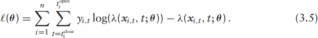
l (θ) = \sum_{i = 1}^{n} \sum_{t = t_{i}^{c lose}}^{t_{i}^{open}} y_{i, t} \log (λ (x_{i, t}, t; θ)) - λ (x_{i, t}, t; θ)

(3.5)

Here, the booking and flight specific intensity in Equation (3.1) is written as a function of the covariates and model parameters as λ( x _i,t,t; θ ). The outer summation is over the number of flights n in the sample, as reported in Table 2, while $t_{i}^{open}$ and $t_{i}^{close}$ are the days to departure at the opening and closing of booking for flight i. For example, if flight i is not cancelled or rescheduled during the 121-day booking window, then these values are $t_{i}^{open}$ = 120 and $t_{i}^{close}$ = 0. Whereas if flight i was cancelled 100 days prior to departure, then $t_{i}^{close}$ = 100.

In Equation (3.5), the covariates are observed on the same resolution as the booking variable, which is the daily level for each flight, which is also the resolution of the revenue management system used by AirABC. Both DTIME and BDAY are observed at this resolution, but the price of a ticket for a given flight can vary between multiple bookings made on the same day so that PRICE is not. In practice, the PRICE variable changes during the day whenever AirABC opens or closes booking classes for a flight mid-way through the day—for example, when a booking class quota is exhausted—and there are 13 988 booking day/flight combinations in our data where this occurs.

To manage intra-day price variation without losing information by averaging the PRICE variable (which could be employed with the likelihood function at Equation (3.5)) and ensure that the predictions are created on a daily level for each flight, we incorporate PRICE variation in the likelihood using differing aggregation levels. For example, if three bookings are observed on a single day, we assume an aggregation level of 1/3 day. This leads to an offset mirroring the aggregation level as described, for instance, in Tutz (2012, Sec. 7.2). To specify this here, let

x_{i, t, l} = ({DTIME}_{i}, {BDAY}_{t}, P R I C E_{i, t, l}),

Table 2

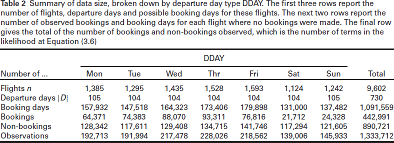
Summary of data size, broken down by departure day type DDAY. The first three rows report the number of flights, departure days and possible booking days for these flights. The next two rows report the number of observed bookings and booking days for each flight where no bookings were made. The final row gives the total of the number of bookings and non-bookings observed, which is the number of terms in the likelihood at Equation (3.6)

	DDAY
Number of …	Mon	Tue	Wed	Thr	Fri	Sat	Sun	Total
Flights n	1,385	1,295	1,435	1,528	1,593	1,124	1,242	9,602
Departure days \|D\|	105	104	104	104	104	104	105	730
Booking days	157,932	147,518	164,323	173,406	179,898	131,000	137,482	1,091,559
Bookings	64,371	74,383	88,070	93,311	76,816	21,712	24,328	442,991
Non-bookings	128,342	117,611	129,408	134,715	141,746	117,294	121,605	890,721
Observations	192,713	191,994	217,478	228,026	218,562	139,006	145,933	1,333,712

be the covariate vector for the lth booking made t days to departure for flight i, where l = 1, …, max(1, y_i,t). On days without any bookings for flight i (i.e., when y_i,t = 0), let 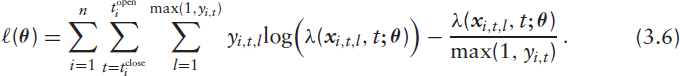x _i,t,1 be the vector of covariate values, and set y_i,t,₁ = 0. Similarly, let y_i,t,l = 1 for l = 1, …, max(1, y_i,t) for days with observed bookings (that is, when y_i,t 1). Then, the (unpenalized) log-likelihood with an aggregation offset is as follows:

l (θ) = \sum_{i = 1}^{n} \sum_{t = t_{i}^{lose}}^{t_{i}^{open}} \sum_{l = 1}^{\max (1, y_{i, t})} y_{i, t, l} \log (λ (x_{i, t, l}, t; θ)) - \frac{λ (x_{i, t, l}, t; θ)}{\max (1, y_{i, t})} .

(3.6)

The multiple summation in Equation (3.6) is over all observed bookings, plus the booking days where no bookings were made for the i th flight (i.e., all instances where y_i,t = 0).

These summations are over all flights i that depart on each given day type. The bottom row of Table 2 reports the number of terms in the summation, and there are between 139 006 and 228 026 of these. Note that if there were no intraday variation in price, then Equations (3.6) and (3.5) would be the same.

Equation (3.6) is augmented with an additive penalty to account for smoothness in the functions. The first and second order derivatives are computed analytically (see Section 5.1 of the Web Appendix) enabling fast direct maximization of the penalized log-likelihood; even for the high sample sizes employed here. The optimal values of these smoothing parameters are selected by minimizing the Bayesian Information Criterion (BIC). The number of latent segments is also selected using BIC, where we fit models with increasing number of segments K as long as this decreases the BIC as in Allenby and Rossi (1998). Bootstrap confidence intervals for the parameters and functions of a fitted model are computed using the ‘leave out one individual’ approach of Rice and Silverman (1991). The identification of the segment labels in the mixture model is achieved by ordering the segment specific price coefficients α_k in a monotone sequence. We refer to Section 6 of the Web Appendix for details.

We comment briefly on the suitability of selecting the number of latent segments using BIC. Whittaker and Miller (2021) explores the accuracy of enumerating the number of classes using different metrics in latent class analysis. They found strong evidence to suggest that sample size adjusted BIC (NBIC) was more accurate than a variety of alternatives, including cross-validation and BIC. However, the results also show similar enumeration accuracy for BIC and NBIC with an increasing sample size. Because our analysis is based on a large sample of size n 1 109 559, BIC is an accurate metric for latent class enumeration.

3.3 Semiparametric regression for price

Treating price as an exogenous variable in a consumer demand model can lead to biased estimates of price elasticity; see discussions in Davidson and MacKinnon (1999, 1993), Wooldridge (2002), Petrin and Train (2010) and references therein. For example, Mumbower et al. (2014) show the importance of controlling for price endogeneity in a linear model for flight bookings using a two-stage least squares linear regression estimator, whereas Lurkin et al. (2017) do so for a choice model. For generalized non-linear models, Marra and Radice (2011) suggest an extension of such two-stage estimators, similar to the control function approach of Petrin and Train (2010). We follow these authors and first build a non-linear model for price based on an instrumental variable and then include the price residual as a covariate in our model of passenger demand.

To do so, we model the logarithm of prices at the daily and flight level as

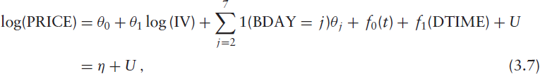
\log (PRICE) = θ_{0} + θ_{1} \log (IV) + \sum_{j = 2}^{7} 1 (BDAY = j) θ_{j} + f_{0} (t) + f_{1} (DTIME) + U = η + U,

(3.7)

where U N(0,σ ²). The effects of t and DTIME are captured by unknown smooth functions f₀ and f₁ modelled by penalized splines, while IV is an instrumental variable.

Mumbower et al. (2014) discusses possible choices for IV and suitable candidates. Li et al. (2014) notes that many candidates are invalid because both the IV and booking data need to be observed at the same level of aggregation to control effectively for price endogeneity. Supply shifters—for example, airport fees, transportation taxes and fuel costs—are constant over daily bookings. Hausman-style instruments at the firm level do not match to a model on the market level. Stern-type instruments that measure competition and market share do not vary on the booking level. Last, IVs that have an impact on marginal costs remain a feasible option, which is why we use (the logarithm of) a variable that is popular in the revenue management literature called the ‘bid-price’ (Talluri and van Ryzin, 2004, p. 31). The bid-price is a measure of the (marginal) cost of offering a seat, taking into account that it cannot be sold again. Crucially, it varies between bookings because the airline updates its assessment frequently. The bid-price is available for all flights in the database and at all time points, as well as for predictive purposes, that is for flights that are yet to depart.

Figure 3

Description of two airline-network scenarios. On the left-hand side, the airline controls for capacity constraints only taking passenger demand from the origin (BBB) to the destination (AAA) into account. Low-cost-carriers typically use this set-up. On the right-hand side, the airline controls for the capacity constraint on the BBB to AAA route by taking all possible passenger demand streams coming from other origins than BBB (arrows going into BBB) to different destinations than AAA (arrows going out of AAA) into account. Network-carriers typically use this set-up

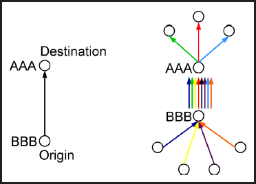
To ensure the validity of our choice the IV needs to fulfill the properties of relevance and exogeneity (Guevara, 2018). Whereas (strong) relevance can easily be demonstrated by the strong non-linear dependence between the IV and the endogenous variable price, exogeneity needs to be addressed by a statistical (over-identification) test. Unfortunately, this test requires the availability of at least two instruments, so that exogeneity cannot be established definitively. From a qualitative perspective, the bid-price is a measurement of displacement cost, ensuring that revenue gain for the available airlines’ network capacity is maximized. As pointed out by Li et al. (2014), the exogeneity (and hence the validity of the bid-price IV) means that a demand shock for flight i at time to departure t (i.e., ε_i (t) Y_i (t) λ_i (t)) is uncorrelated with the IV. Figure 3 describes two possible revenue management setups, where an airline only controls for displacement cost on route-level (left-hand side) or incorporates all possible demand-streams into the displacement cost calculation (right-hand side). As AirABC is a network carrier, it considers every demand stream when calculating the bid-price value. Therefore, the bid-price defines the distribution of all network demand on the route. In our study, the share of transfer passengers, that is passengers not travelling solely between BBB and AAA, is approximately 50%. Thus, the bid-price value is largely determined by factors that are exogenous to the route under study. Hence, we conclude that the demand shock ε_i (t) and the bid-price are uncorrelated.

We fit the model at Equation (3.7) using maximum likelihood, and then use this to estimate the error

ξ = PRICE - E (PRICE ∣ IV,BDAY,t,DTIME) = PRICE - \exp (η + σ^{2} / 2)

Table 3

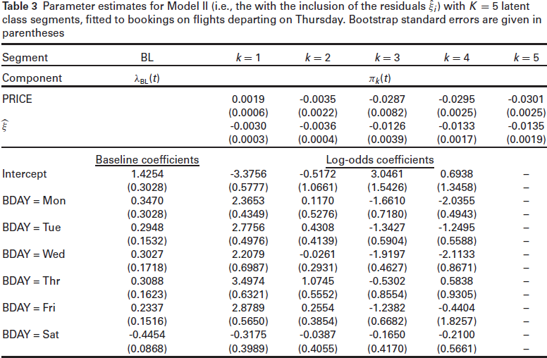
Parameter estimates for Model II (i.e., the with the inclusion of the residuals ξˆi) with K = 5 latent class segments, fitted to bookings on flights departing on Thursday. Bootstrap standard errors are given in parentheses

Segment	BL	k = 1	k = 2	k = 3	k = 4	k = 5
Component	λ_BL(t)	π_k(t)
PRICE		0.0019	-0.0035	-0.0287	-0.0295	-0.0301
		(0.0006)	(0.0022)	(0.0082)	(0.0025)	(0.0025)
$\hat{ξ}$		-0.0030	-0.0036	-0.0126	-0.0133	-0.0135
		(0.0003)	(0.0004)	(0.0039)	(0.0017)	(0.0019)
Baseline coefficients			Log-odds coefficients
Intercept	1.4254	-3.3756	-0.5172	3.0461	0.6938	–
	(0.3028)	(0.5777)	(1.0661)	(1.5426)	(1.3458)	–
BDAY = Mon	0.3470	2.3653	0.1170	-1.6610	-2.0355	–
	(0.3028)	(0.4349)	(0.5276)	(0.7180)	(0.4943)	–
BDAY = Tue	0.2948	2.7756	0.4308	-1.3427	-1.2495	–
	(0.1532)	(0.4976)	(0.4139)	(0.5904)	(0.5588)	–
BDAY = Wed	0.3027	2.2079	-0.0261	-1.9197	-2.1133	–
	(0.1718)	(0.6987)	(0.2931)	(0.4627)	(0.8671)	–
BDAY = Thr	0.3088	3.4974	1.0745	-0.5302	0.5838	–
	(0.1623)	(0.6321)	(0.5552)	(0.8554)	(0.9305)	–
BDAY = Fri	0.2337	2.8789	0.2554	-1.2382	-0.4404	–
	(0.1516)	(0.5650)	(0.3854)	(0.6682)	(1.8257)	–
BDAY = Sat	-0.4454	-0.3175	-0.0387	-0.1650	-0.2100	–
	(0.0868)	(0.3989)	(0.4055)	(0.4170)	(0.5661)	–

for each flight and booking day combination. The resulting residuals values are observations on the covariate $\hat{ξ}$ , which is included in the log-linear segment price adjustments, so that we replace Equation (3.3) by

\log (δ_{k}) = α_{1, k} PRICE + α_{2, k} \hat{ξ} .

(3.8)

We will subsequently refer to Model I if we ignore endogeneity and use Equation (3.3). Taking endogeneity into account and using Equation (3.8) is referred to as Model II. A more detailed motivation for this two-stage procedure using the bid-price as an instrumental variable is given in Section 7 of the Web Appendix.

4 Empirical analysis

We now discuss the estimates from our model. Because we fit it to bookings for flights departing on different day types—that is, different values of DDAY—separately, we give in detail the results arising from flights departing on Thursday. This is the departure day with the highest demand.

Figure 4

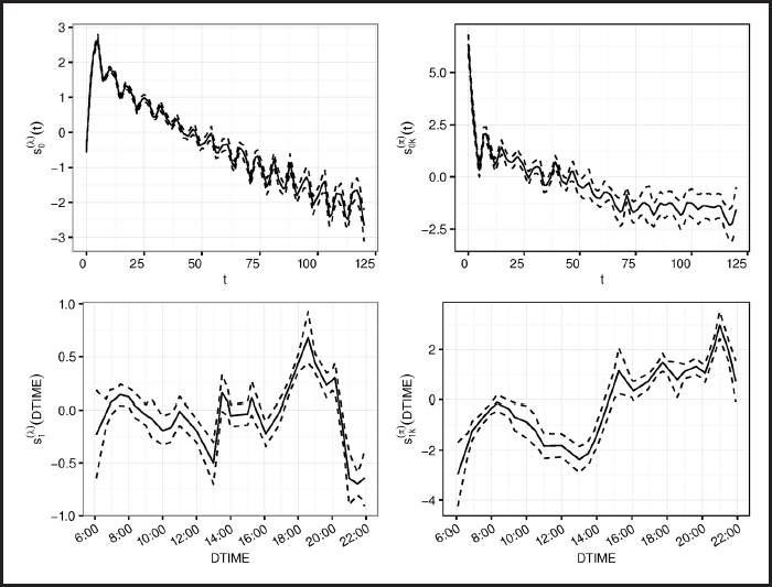
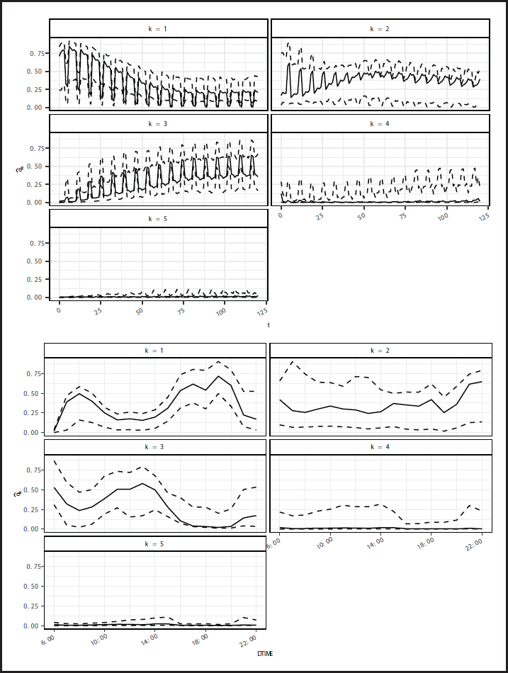
For K = 5 segments, the left-hand panels provide the function estimates for $s_{0}^{(λ)} (t)$ and $s_{1}^{(λ)} (DTIME)$ in Equation (3.2) for bookings on flights that depart on Thursday. The right-hand side shows the estimates of $s_{0, k}^{(π)} (t)$ and $s_{1, k}^{(π)} (DTIME)$ , k = 1,…, 4 in Equation (3.4). The first-stage residuals $\hat{ξ}$ are included (i.e. Model II). The estimates are given by the solid line, while the dashed lines are 99% local confidence bands

We fit the demand models with K = 2, …, 7 segments, both including and excluding the price model residuals $\hat{ξ}$ (the calculation of $\hat{ξ}$ is discussed in Section 2 of the Web Appendix). The inclusion of the residuals improves the fit of the demand models substantially—as measured using either AIC or BIC—in every case. A detailed discussion of the K 2 segment model estimates, and the impact of controlling for endogeneity, is given in Section 3 of the Web Appendix. For all seven departure days (DDAY), Table 5 reports the BIC values for all fitted demand models that include the residuals $\hat{ξ}$ and different numbers of segments. For flights departing on Thursday (DDAY = Thr), K 5 segments are optimal with the minimum BIC value. Table 3 gives the estimates of the linear coefficients. Inclusion of the price residual has a substantial effect on the parameter estimates so that we subsequently only discuss the results with price endogeneity taken into account. The segment adjustment coefficients shows that the PRICE coefficient for segment 2 is insignificant and close to insignificant for segment 1. However, segments 3, 4, and 5 exhibit significant price sensitivities between ${\hat{α}}_{3} = - 0.0287$ and ${\hat{α}}_{5} = - 0.0301$ .

Figure 4 shows the fitted smooth terms of model component at Equation (3.2) (left panel) and Equation (3.4) (right panel). We see a general increase in demand closer to the day of departure (i.e., for lower values of t). Moreover, the size of segments 1 and 4 increase, and segment 3 decreases, closer to the day of departure. Segment 2 shows no significant time effect. DTIME has only a weak impact on demand, although this is not the case for customer segmentation which we discuss next.

To measure the composition of customers as a function of time to departure, we compute the ratio

q_{k} (t) = \frac{π_{k} (t) δ_{k}}{\sum_{k^{'} = 1}^{K} π_{k^{'}} (t) δ_{k^{'}}},

(4.1)

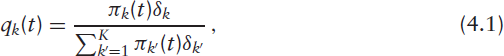
for k = 1, 2, …, K. This ratio measures the proportion of customers in segment k. In our demand model, the component π_k(t) is a function of both flight and booking level covariates, so that we compute the mean ${\bar{q}}_{k} (t)$ by averaging q_k(t) over all flights and bookings on a given day to departure t.

Figure 5 (top panel) plots ${\bar{q}}_{k} (t)$ for the five segments against days to departure. Only a very small proportion of bookings fall into the price-sensitive segments 4 and 5. For segment 5 passengers arrive anytime, whereas segment 4 corresponds to a type of passenger that arrives shortly before departure. The vast bulk of bookings by price-sensitive customers are in segment 3. This accounts for around 40%–50% of all bookings made up to 75 days before departure, but gradually declines as the flight departure approaches, falling to almost none in the week prior to departure. Bookings made in this segment are also more likely to be made on the weekend (i.e., when BDAY is either Saturday or Sunday). The proportion of bookings that fall into the two price inelastic segments have quite different patterns. The probability of a booking in segment 1 is at most 20% until 75 days prior to departure, after which it increases rapidly until the day of departure, during which just over 80% of bookings arise from this segment. Bookings in segment 2 are common throughout the booking window, varying between around 20% to 60% of the total. Interestingly, bookings in this segment exhibit a strong booking day effect—with bookings much more likely on the weekend than weekdays—a stark difference with bookings in segment 1 which do not.

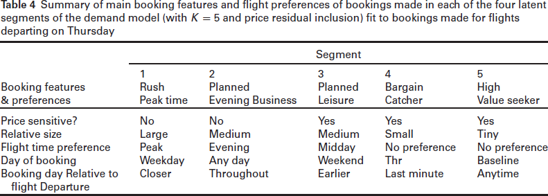
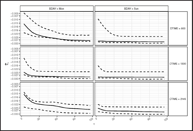
The probability π_k of being in segment k is also a function of DTIME through the MNL model at Equation (3.4). Thus, the diagnostic ratio can be also be computed as a function of DTIME, which we write as ${\bar{q}}_{k} (DTIME)$ . The bottom panel in Figure 5 plots this ratio against DTIME for each of the five segments. Of the two price-insensitive latent classes, segment 1 accounts for around 50% of all bookings on fights departing during the morning peak, and a striking 70% of those during the evening peak. In contrast, segment 2 bookings exhibit a preference for the late evening. Bookings in the price-sensitive segment 3 are largely for flights departing during off-peak periods, whereas segment 4 and 5 show no particular time preference.

Table 4 summarizes the main features of each latent segment, which we label as ‘Rush Peak-time’ (segment 1), ‘Planned Evening Business’ (segment 2), ‘Planned Leisure’ (segment 3), ‘Bargain Catcher’ (segment 4) and ‘High Value Seeker’ (segment 5). We also compute the overall elasticity estimate E_λ that averages over the latent segments. Figure 6 plots E_λ against the time to departure for select values of DTIME and BDAY. All panels show that the price elasticity decreases as the day of departure nears (t 0). This effect is stronger for a weekday booking day, for example Monday, compared to a weekend booking day such as Sunday. In the weeks immediately prior to departure, tickets on morning and evening flights are much more price inelastic than tickets for midday flights. Overall, the results indicate that K 5 passenger segments successfully identify customer heterogeneity in price elasticity broken down by time to departure (t) and departure time (DTIME), allowing for optimal variable pricing of tickets.

Figure 5

Plot of the average segment proportion computed from the model fitted to booking on flights departing on Thursday and K 5 (solid line) with 99% local bootstrapped confidence bands (dashed lines). Top row: within each panel, ${\bar{q}}_{k} (t)$ is plotted against days to departure t. Bottom row: within each panel, ${\bar{q}}_{k} (DTIME)$ is plotted against DTIME

Table 4

Summary of main booking features and flight preferences of bookings made in each of the four latent segments of the demand model (with K 5 and price residual inclusion) fit to bookings made for flights departing on Thursday

			Segment
	1	2	3	4	5
Booking features	Rush	Planned	Planned	Bargain	High
& preferences	Peak time	Evening Business	Leisure	Catcher	Value seeker
Price sensitive?	No	No	Yes	Yes	Yes
Relative size	Large	Medium	Medium	Small	Tiny
Flight time preference	Peak	Evening	Midday	No preference	No preference
Day of booking	Weekday	Any day	Weekend	Thr	Baseline
Booking day Relative to flight Departure	Closer	Throughout	Earlier	Last minute	Anytime

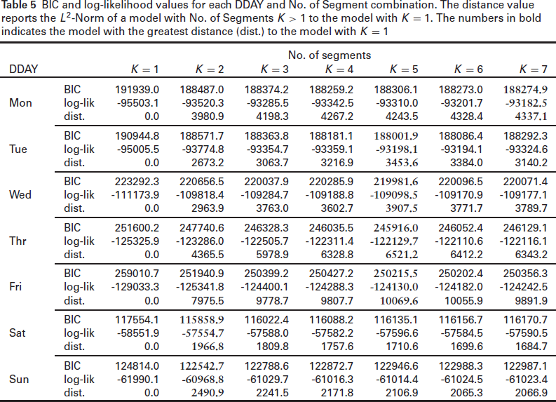
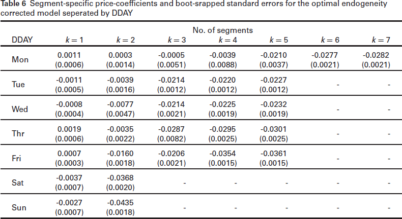
So far we have looked at Thursday departures only. We extend this now and fit the demand model to bookings for flights on all departure days. The BIC values for K 1,…, 7 customer segments are shown in Table 5, while the corresponding estimated coefficients of PRICE for the optimal model based on the BIC are reported in Table 6. For weekday departures (except Monday) K = 5 is optimal throughout, and the segment specific price sensitivities are similar across departure day.

For example, there are two price-insensitive segments, with the exception of Friday flights where there is only one. For flights departing during the weekend the optimal number of segments is K = 2, indicating less customer heterogeneity. For all seven departure days, the individual segments exhibit significant differences in price elasticity, which can be exploited for variable pricing purposes.

In Section 4 of the Web Appendix, we validate the assumption of conditional independence of flight counts during a departure day. To do so, we extend the univariate model to a multivariate Poisson model to analyse possible dependencies between flights. No significant dependence between flights is found, and we conclude that the proposed mixture-of-experts model is unbiased by unobserved heterogeneity caused by additional dependence between demand for flights departing on the same day.

Table 5

BIC and log-likelihood values for each DDAY and No. of Segment combination. The distance value reports the L²-Norm of a model with No. of Segments K > 1 to the model with K = 1. The numbers in bold indicates the model with the greatest distance (dist.) to the model with K = 1

		No. of segments
DDAY		K = 1	K = 2	K = 3	K = 4	K = 5	K = 6	K = 7
	BIC	191939.0	188487.0	188374.2	188259.2	188306.1	188273.0	188274.9
Mon	log-lik	-95503.1	-93520.3	-93285.5	-93342.5	-93310.0	-93201.7	-93182.5
	dist.	0.0	3980.9	4198.3	4267.2	4243.5	4328.4	4337.1
	BIC	190944.8	188571.7	188363.8	188181.1	188001.9	188086.4	188292.3
Tue	log-lik	-95005.5	-93774.8	-93354.7	-93359.1	-93198.1	-93194.1	-93324.6
	dist.	0.0	2673.2	3063.7	3216.9	3453.6	3384.0	3140.2
	BIC	223292.3	220656.5	220037.9	220285.9	219981.6	220096.5	220071.4
Wed	log-lik	-111173.9	-109818.4	-109284.7	-109188.8	-109098.5	-109170.9	-109177.1
	dist.	0.0	2963.9	3763.0	3602.7	3907.5	3771.7	3789.7
	BIC	251600.2	247740.6	246328.3	246035.5	245916.0	246052.4	246129.1
Thr	log-lik	-125325.9	-123286.0	-122505.7	-122311.4	-122129.7	-122110.6	-122116.1
	dist.	0.0	4365.5	5978.9	6328.8	6521.2	6412.2	6343.2
	BIC	259010.7	251940.9	250399.2	250427.2	250215.5	250202.4	250356.3
Fri	log-lik	-129033.3	-125341.8	-124400.1	-124288.3	-124130.0	-124182.0	-124242.5
	dist.	0.0	7975.5	9778.7	9807.7	10069.6	10055.9	9891.9
	BIC	117554.1	115858.9	116022.4	116088.2	116135.1	116156.7	116170.7
Sat	log-lik	-58551.9	-57554.7	-57588.0	-57582.2	-57596.6	-57584.5	-57590.5
	dist.	0.0	1966.8	1809.8	1757.6	1710.6	1699.6	1684.7
	BIC	124814.0	122542.7	122788.6	122872.7	122946.6	122988.3	122987.1
Sun	log-lik	-61990.1	-60968.8	-61029.7	-61016.3	-61014.4	-61024.5	-61023.4
	dist.	0.0	2490.9	2241.5	2171.8	2106.9	2065.3	2066.9

Table 6

Segment-specific price-coefficients and boot-srapped standard errors for the optimal endogeneity corrected model seperated by DDAY

	No. of segments
DDAY	k = 1	k = 2	k = 3	k = 4	k = 5	k = 6	k = 7
Mon	0.0011	0.0003	-0.0005	-0.0039	-0.0210	-0.0277	-0.0282
Mon	(0.0006)	(0.0014)	(0.0051)	(0.0088)	(0.0037)	(0.0021)	(0.0021)
Tue	-0.0011	-0.0039	-0.0214	-0.0220	-0.0227	-	-
Tue	(0.0005)	(0.0016)	(0.0012)	(0.0012)	(0.0012)	-	-
Wed	-0.0008	-0.0077	-0.0214	-0.0225	-0.0232	-	-
Wed	(0.0004)	(0.0047)	(0.0021)	(0.0019)	(0.0019)	-	-
Thr	0.0019	-0.0035	-0.0287	-0.0295	-0.0301	-	-
Thr	(0.0006)	(0.0022)	(0.0082)	(0.0025)	(0.0025)	-	-
Fri	0.0007	-0.0160	-0.0206	-0.0354	-0.0361	-	-
Fri	(0.0003)	(0.0018)	(0.0021)	(0.0015)	(0.0015)	-	-
Sat	-0.0037	-0.0368	-	-	-	-	-
Sat	(0.0007)	(0.0020)	-	-	-	-	-
Sun	-0.0027	-0.0435	-	-	-	-	-
Sun	(0.0007)	(0.0018)	-	-	-	-	-

Figure 6

Estimated overall price elasticity E_λ (solid line) for a mixture of K = 5 customer segments, estimated with endogeneity correction. Also plotted are 99% local bootstrapped confidence bands (dashed lines). Six combinations of booking day (BDAY) and departure time (DTIME) are considered, and days to departure (t) is on the horizontal axis

5 Conclusion

We propose a flexible non-homogeneous Poisson model of demand for passenger flights and apply it to a large dataset constructed from the booking database of a major airline. The dataset contains daily booking counts for all flights on a single busy short-haul route, where the airline has no direct competition. In comparison to most previous studies, our data do not suffer from the exclusions typical of data constructed either using web crawlers or sourced from the Global Distribution System. Our empirical study reveals four substantive findings with managerial and marketing implications for airlines.

First, based on the BIC criteria (see, Table 5), our latent segmentation model suggests that there are typically between two and five consumer segments, which have very different levels of price elasticity. Using an MNL model, we show that the probability of segment membership varies substantially over the flight departure time, booking day type and number of days to departure at the time of booking in a non-linear way, so that price elasticity does so also. Quantifying variable price elasticities, as a mixture of passenger segments, is essential for revenue management practices where the airlines try to maximize their revenue by optimally changing the price of a ticket. From a marketing perspective, the characterization of customer segments in Table 4 allows AirABC to better tailor its product and promotion activities.

Second, we consider a booking horizon of 120 days, which is longer than in most previous studies. During this period, as seen by the varying segment proportions of Figure 5, we find the determinants of demand (and elasticity) vary greatly, suggesting that continuous tailoring of price and marketing over the entire booking horizon is warranted.

Third, the covariates used in our model are all fully observable throughout the airline scheduling horizon of 365 days before departure and allow for forecasting of elasticity and demand for use in airlines’ revenue management systems. In contrast, capturing consumer heterogeneity using individual customer level data that includes some customer characteristics would not allow for forecasting future demand and price elasticity because this data is typically unknown to the airline at the time of booking. Moreover, retention of individual-level customer data is likely to be increasingly difficult under data privacy provisions, such as the EU GDPR.

Last, we highlight the importance of accounting for endogeneity when estimating price elasticity. While studies have shown this previously for aggregate data, we do so at a disaggregate level within a flexible mixture-of-experts framework with non-linear effects captured using regularized splines. A control variate approach is used with the bid-price as an instrument, which is discussed in detail for two latent passenger segments in Section 3 of the Web Appendix. The advantage of using the bid-price is that it varies at the same resolution as our booking data—that is at the flight and daily level—and proves to be a strong instrument.

Our study uses data from customers purchasing published fares for the economy class cabin on a single route without any competition from other airlines. The advantage of focusing on this specific situation is that it can be seen as a controlled experiment. Nevertheless, the model developed is applicable more generally. It has been applied by AirABC to bookings on other routes with competitors and a varying share of passengers who buy published fares. To model and forecast demand in those scenarios, additional variables are simply added to describe the behaviour of competitors and passenger segments.

The extension of the model to a multivariate Poisson model using a Gaussian copula, as outlined in Section 4 of the Web Appendix, has strong potential. While we found little evidence of additional dependence between bookings on flights that depart on the same day, it can also be used to capture dependence between other bookings. For example, between bookings for (a) the same flight on adjacent days (which would be a type of longitudinal model) and (b) different flights departing during the same hourly period but in adjacent days. Such analyses would enable a better understanding of how price variation at the flight and daily level affect demand for substitute flights and provide a step towards improved continuous pricing by airlines.

Our research was undertaken before the 2020 COVID-19 pandemic, which at the time of writing, has greatly affected flights around the world. However, as air travel resumes the insights listed above are likely to remain valid. This is because our statistical model has interpretable components, whereas black-box models (e.g., deep neural networks) are often difficult to extrapolate in the presence of a structural shock. We conclude by noting that prior to March 2020, insights from these results were incorporated into practice by AirABC. Tickets on the considered route, as well as on comparable connections, were priced based on the proposed model. As air travel recovers post-COVID-19, AirABC will likely continue to price tickets using this model, while incorporating adjustments to key components (notably the baseline intensity) to reflect new demand realities as they emerge.

Footnotes

Declaration of Conflicting Interests

The authors declared no potential conflicts of interest with respect to the research, authorship and/or publication of this article.

Funding

The authors received no financial support for the research, authorship and/or publication of this article.

References

Allenby

, and Rossi

(1998) Marketing models of consumer heterogeneity. Journal of Econometrics , 89, 57–78.

Davidson

, and MacKinnon

(1993) Estimation and Inference in Econometrics , 1st edition. Oxford: Oxford University Press.

Davidson

, and MacKinnon

(1999) Econometric Theory and Methods . 1st edition. Oxford: Oxford University Press.

Diaconescu

(2008) The use of NARX neural networks to predict chaotic time series. Wseas Transactions on computer research , 3, 182– 191.

Eilers

, and Marx

(1996) Flexible Smoothing with B-Splines and Penalties. Statistical Science , 11, 89–121.

Escobari

(2017) Airport, airline and departure time choice and substitution patterns: An empirical analysis. Transportation Research A , 103, 198–210.

Guevara

(2018) Overidentification tests for the exogeneity of instruments in discrete choice models. Transportation Research B , 114, 241–253.

Hastie

, and Tibshirani

(1990) Generalized Additive Models. London: Chapman & Hall.

Hetrakul

, and Cirillo

(2014) A latent class choice based model system for railway optimal pricing and seat allocation. Transportation Research E , 61, 68–83.

10.

IATA (2020a) After Challenging Year, Improvement Expected for 2020 . https://www.iata.org/en/pressroom/pr/2019-12-11-01/ (accessed at 2020-07-08).

11.

IATA (2020b) 2036 Forecast reveals air passengers will nearly double to 7.8 billion . https://www.iata.org/en/pressroom/pr/2017-10-24-01/ (accessed at 2020-07-08).

12.

Jordan

, and Jacobs

(1994) Hierarchical mixtures of experts and the em algorithm. Neural computation , 6, 181–214.

13.

Karlis

, and Xekalaki

(2005) Mixed poisson distributions. International Statistical Review , 73, 35–58.

14.

Kauermann

, Krivobokova

, and Fahrmeir

(2009) Some asymptotic results on generalized penalized spline smoothing. Journal of the Royal Statistical Society, Series B , 71, 487–503.

15.

, Zheng

, Yang

, and Chen

(2017) Short-term forecasting of passenger demand under on-demand ride services: A spatiotemporal deep learning approach. Transportation Research C , 85, 591–608.

16.

, Granados

, and Netessine

(2014) Are consumers strategic? structural estimation from the air-travel industry. Management Science , 60, 2114–2137.

17.

Lin

, He

, and Peeta

(2018) Predicting station-level hourly demand in a large-scale bike-sharing network: A graph convolutional neural network approach. Transportation Research C , 97, 258–276.

18.

Lurkin

, Garrow

, Higgins

, Newman

, and Schyns

(2017) Accounting for price endogeneity in airline itinerary choice models: An application to continental us markets. Transportation Research A , 100, 228–246.

19.

Marra

, and Radice

(2011) A flexible instrumental variable approach. Statistical Modelling , 11, 581–603.

20.

Mumbower

, Garrow

, and Higgins

(2014) Estimating flight-level price elasticities using online airline data: A first step toward integrating pricing, demand, and revenue optimization. Transportation Research A , 66, 196–212.

21.

Peterson

, and Thankom

(2020) Spillover of COVID-19: Impact on the global economy (MPRA Paper No. 99317). URL https://ideas.repec.org/p/pra/mprapa/99317.html(last accessed 23 February 2022).

22.

Petrin

, and Train

(2010) A control function approach to endogeneity in consumer choice models. Journal of Marketing Research , 47, 3–13.

23.

Rice

, and Silverman

(1991) Estimating the mean and covariance structure nonparametrically when the data are curves. Journal of the Royal Statistical Society, Series B , 53, 233–243.

24.

Ruppert

, Wand

, and Carroll

(2003) Semiparametric Regression . Cambridge: Cambridge University Press.

25.

Ruppert

, Wand

, and Carroll

(2009) Semiparametric regression during 2003–2007. Electronic Journal of Statistics , 3, 1193–1256.

26.

Smith

, and Kauermann

(2011) Bicycle commuting in melbourne during the 2000s energy crisis: A semiparametric analysis of intraday volumes. Transportation Research B , 45, 1846–1862.

27.

Talluri

, and van Ryzin

(2004) Revenue management under a general discrete choice model of consumer behavior. Management Science , 50, 15–33.

28.

Talluri

, and van Ryzin

(2005) The Theory and Practice of Revenue Management. International Series in Operations Research & Management Science . Berlin: Springer.

29.

Teichert

, Shehu

, and von Wartburg

(2008) Customer segmentation revisited: The case of the airline industry. Transportation Research A , 42, 227–242.

30.

Tutz

(2012) Regression for Categorical Data . Cambridge: Cambridge University Press.

31.

Vulcano

, van Ryzin

, and Chaar

(2010) Choice-based revenue management: An empirical study of estimation and optimization. Manufacturing & Service Operations Management , 12, 371–392.

32.

Wedel

, and Kamakura

(2012) Market Segmentation: Conceptual and Methodological Foundations, Volume 8 . Berlin: Springer Science & Business Media.

33.

C-H

Wen

, and P-H

Chen

(2017) Passenger booking timing for low-cost airlines: A continuous logit approach. Journal of Air Transport Management , 64, 91–99.

34.

C-H

Wen

, and S-C

Lai

(2010) Latent class models of international air carrier choice. Transportation Research E , 46, 211–221.

35.

Whittaker

, and Miller

(2021) Exploring the enumeration accuracy of cross-validation indices in latent class analysis. Structural Equation Modelling: A Multidisciplinary Journal , 28, 376–390.

36.

Wood

(2017) Generalized Additive Models: An Introduction with R. Chapman & Hall, CRC Texts in Statistical Science . Boca Raton, FL: CRC Press.

37.

Wooldridge

(2002) Introductory Econometrics: A Modern Approach , 2nd edition. Nashville, TN: SouthWestern.

38.

, Ji

, and Liu

(2018) The station-free sharing bike demand forecasting with a deep learning approach and large-scale datasets. Transportation Research C , 95, 47–60.