
Abstract
This article studies long-term, short-term volatility and co-volatility in stock markets by introducing modelling strategies to the multivariate data analysis that deal with serially correlated innovations and cross-section dependence. In particular, it presents an innovative mixed-effects model through a GARCH process, allowing for heterogeneity effects and time-series dynamics. We propose a non-parametric regression model of the penalized low-rank smoothing spline to present time trends into the variance and covariance equations. The strategy provides flexible modelling of the low-frequency volatility and co-volatility in equity markets. The decomposed low-frequency matrix was modelled using the modified Cholesky factorization. The Hamiltonian Monte Carlo technique is implemented as a Bayesian computing process for estimating parameters and latent factors. The advantage of our modelling strategy in empirical studies is highlighted by examining the effect of latent financial factors on a panel across 10 equities over 110 weekly series. The model can differentiate non-parametrically dynamic patterns of high and low frequencies of variance–covariance structural equations and incorporate economic features to predict variabilities in stock markets regarding time-series evidence.
Keywords
Introduction
Most effort in the literature of financial and economic multivariate data with serially correlated time-series has been devoted to the slow-moving variation and covariation topics. Related studies have frequently been centred on the long-run variation. For example, Engle and Rangel (2008) introduced a notable spline-GARCH model for low-frequency volatility and global macroeconomic events. Audrino and Bühlmann (2009) offered a spline regression model in the non-parametric setting to predict the volatility of financial time-series. Some useful strategies rendering high-performance model fittings are introduced to mixed modelling with smoothing splines (Wahba (1990); Eilers and Marx (1996); Wand (2003)). Speckman and Sun (2003) applied full Bayesian smoothing splines, thin-plate splines, L-splines and several models using intrinsic autoregressive priors. Vogt and Linton (2017) investigated the longitudinal data analysis with non-parametric regression functions in the case of varying individual-specific effects.
The treatment of volatilities is conventionally based on variances, while the modelling of covariance functions can provide better representation. It is reasonable since the volatility in a market can cause volatility in other markets. Thus, most research recommends fitting the multivariate generalized autoregressive conditional heteroscedastic (MGARCH) model. It can describe the volatility in financial markets and efficiently estimate large time-varying covariance matrices. Rangel and Engle (2012) characterize the correlation matrix's high- and low-frequency components by combining a factor model with other specifications that capture the dynamic behaviour of volatilities and covariances between a common factor and idiosyncratic returns. Engle and Sokalska (2012) introduced an intra day volatility forecasting model to some assets by decomposing the volatility of high-frequency returns into several components.
Extensions of multivariate GARCH models to cross-sectional time-series data appeal to further investigations since they can conveniently consider volatilities and co-volatilities in correlated cross-section financial data. So far, the existing models’ methodology has been concentrating on volatility using the quadratic-spline method. There is a gap in the literature for flexible low-frequency models to deliver a more precise prediction. These issues motivate us to introduce the spline-GARCH mixed-effects model by extending the univariate case of Engle and Rangel (2008). We study low-frequency changes using semi-parametric mixed-effects models having a time-varying conditional covariance matrix. We let parameters across assets heterogeneous to control possibly correlated, time-invariant and heterogeneity effects.
Frequently, the volatility of an asset affects other assets through conditional covariances over time. We expect that a shock in a market increases the volatility of other associated markets. However, the influence of negative and positive shocks does not lead to the same fluctuation. Our study aims to present the cross-asset dependence between asset returns, which changes over time intervals, and the amount of volatility during a specific period. Our findings reveal that cross-asset dependence may not increase in the long term. It may occur because of the globalization of financial markets. The dependence effect can be investigated directly using cross-section and time-series modelling specified by the dynamic behaviour of covariances or correlations.
In addition to preserving appropriate features of the GARCH model, its time-varying extension can sufficiently isolate high- and low-frequency volatility and co-volatility. This extension leads to coherent predictions since short-term volatility immediately affects the log-return, while long-term volatility possesses a significant role in future transactions. It also helps financial traders with proper forecasting decisions.
We organize the article as follows. In Section 2, we introduce the mixed-effects spline MGARCH model. Section 3 implements an advanced numerical estimation method, so-called Hamiltonian or Hybrid Monte Carlo (HMC), to provide inference. In Section 4, we conducted simulation studies to investigate the main properties of our model and presented an empirical study in predicting low- and high-frequency volatility of log-returns data. Section 5 includes concluding remarks.
Specification of the proposed model
We first specify the heterogeneous MGARCH model and then extend the mixed-effects methodology to time-varying MGARCH models aiming to describe low-frequency volatilities and co-volatilities.
Heterogeneous MGARCH model
For a cross-section of

where the innovation term


for
We now extend mixed-effects modelling of the heterogeneous MGARCH using the spline-GARCH technique while describing low-frequency volatilities and co-volatilities in the equities market. Commonly, stock returns possess time-varying variances and covariances due to daily news intensity that (a) depend on the macroeconomic events or time-varying conditions that some observed covariates can explain, (b) respond to several latent factors that cannot often be recognized, at least without having additional information. Flexible modelling of the low-frequency volatility and co-volatility, say

where the
Similarly,

for

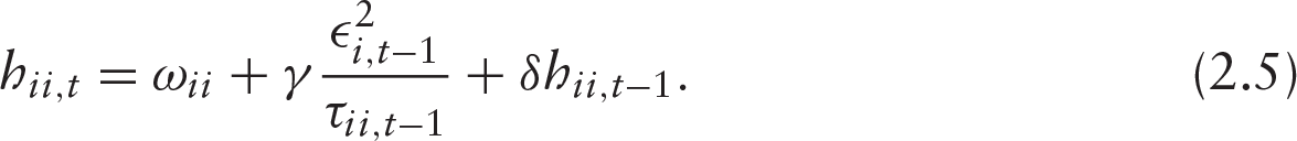
Equation (2.7) provides a well-defined description of co-volatility. We let (2.5) and (2.7) be heterogeneous by assuming random elements

for
The representation of unexpected returns in the vector notation is similar to the familiar MGARCH model, while random effects are present in the model specification. To estimate model parameters in frequentist or Bayesian frameworks, we may face two serious challenges: (a) there is no guarantee that the conditional covariance matrix of innovations,

where

where

where
Now, we present a practical trick to confirm the positive definiteness of the low-frequency matrix. Assume that

for
Denote
We use a penalized splines technique, so-called P-splines (Ruppert et al.(2003); Crainiceanu et al.(2005)). Let two functions
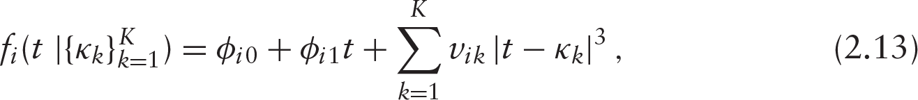
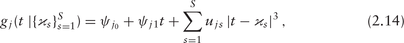
where the regression coefficients
Smoothing splines require a certain background to use suitable spline functions. In practical applications, regression splines yield similar estimates with fewer knots than smoothing splines, particularly when estimated by discrete penalized techniques. Various splines can be formed by altering the choice of knots and changing how roughness in the estimated regression function is penalized. An approach allows a knot at each value of the variable, which, given an appropriate choice of roughness penalty, leads to a natural cubic smoothing spline. It is necessary for fitting regression splines to carefully choose knot locations and basis functions to have subjectivity in the model fitting process. A greater smoothness can be achieved by shrinking the estimated coefficients towards zero.
Let


for Homogeneous intercepts and slopes: Coefficient vectors Heterogeneous intercepts and homogeneous slopes: Coefficient vectors Both intercepts and slopes heterogeneous: Let coefficient vectors
Since the proposed model contains many latent variables, it complicates the estimation process and enforces advanced numerical approaches. The Hamiltonian Monte Carlo is a useful Bayesian computing tool to deal with such issues.
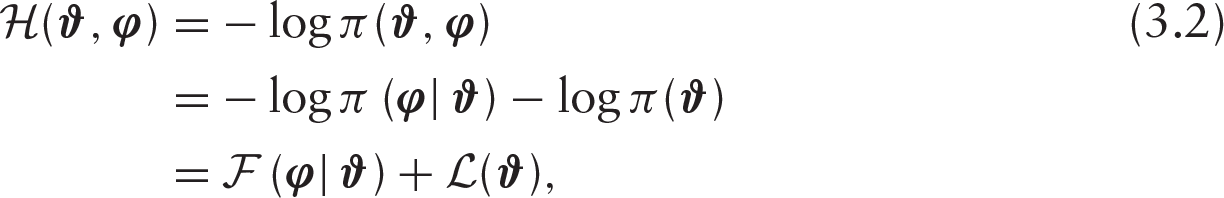
Bayesian computational tools are convenient to fit complex financial models that appear in hierarchical representations. Bayesian inference requires the joint posterior distribution of all unknown model parameters. The conditional density of

For the complete dataset, the conditional likelihood function is
The Bayesian analysis necessities to determine prior distributions for parameters under conditions
To study the impact of heterogeneity on the variance and covariance equations, suppose that random effects matrix,
Prior specification for the low-frequency volatility model
We adopt
Parameter estimation via Hamiltonian Monte Carlo
Hamiltonian Monte Carlo is an effective computational approach (Duane et al.(1987); Neal (1994)) when dealing with complex modelling problems. It uses an approximate Hamiltonian dynamics simulation based on derivatives of density functions to generate an efficient sample from posterior density functions. Neal (2011) and Betancourt and Girolami (2015) detailed some theoretical and practical topics.
Let
where

For the continuous time


where
for some small step-size

otherwise, the previous parameter value is returned for the next draw and used as an initial value for the next iteration. A summary of the HMC algorithm is as follows
initialize parameters, set initial values generate set repeat the leapfrog solution
set compute set let
To perform data analysis of the empirical studies, we employ Stan’s probabilistic programming language, which uses the HMC algorithm. A Stan code is initially compiled to a C++ programme by the facility of Stan compiler, the so-called stanc. Next, a self-contained platform-specific executable recompiles the code. We use the RStan library, the R interface to Stan, see Carpenter et al.(2017), and ‘GitHub,
The posterior predictive distribution (PPD) has often been used to check model performance. For
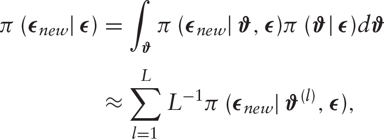
where
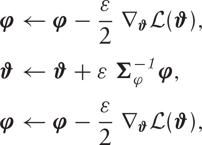
Optimization-based inference
Denoting
where
Simulation and empirical application
We first conduct simulation studies to investigate the statistical properties of the time-varying GARCH mixed-effects model and then analyse the stock market dataset to model volatility and co-volatility.
Simulation experiments
We simulate the unexpected returns, conditioned on latent variables and innovation terms, and generate some proposed time-varying multivariate model paths. Financial time-series data exhibit specific features that should be included in the simulation study. Specifically, the simulated series variability is taken into account by time-varying coefficients. We expect that non-stationary processes with high variation intend extreme peaks. Also, variance components control volatility and co-volatility in the sample paths.
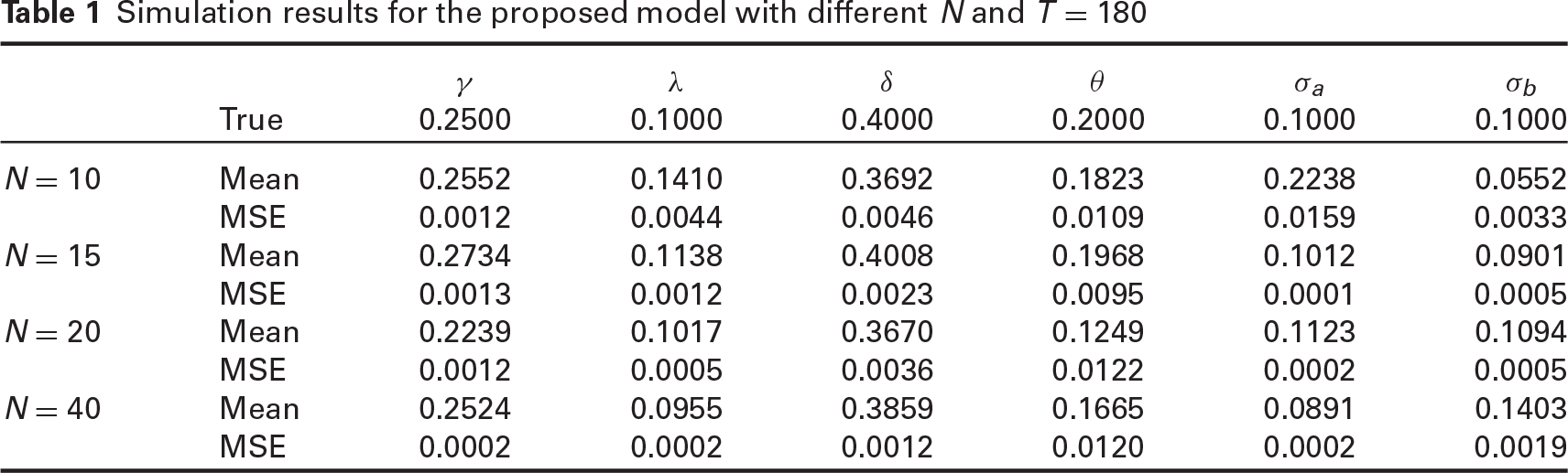
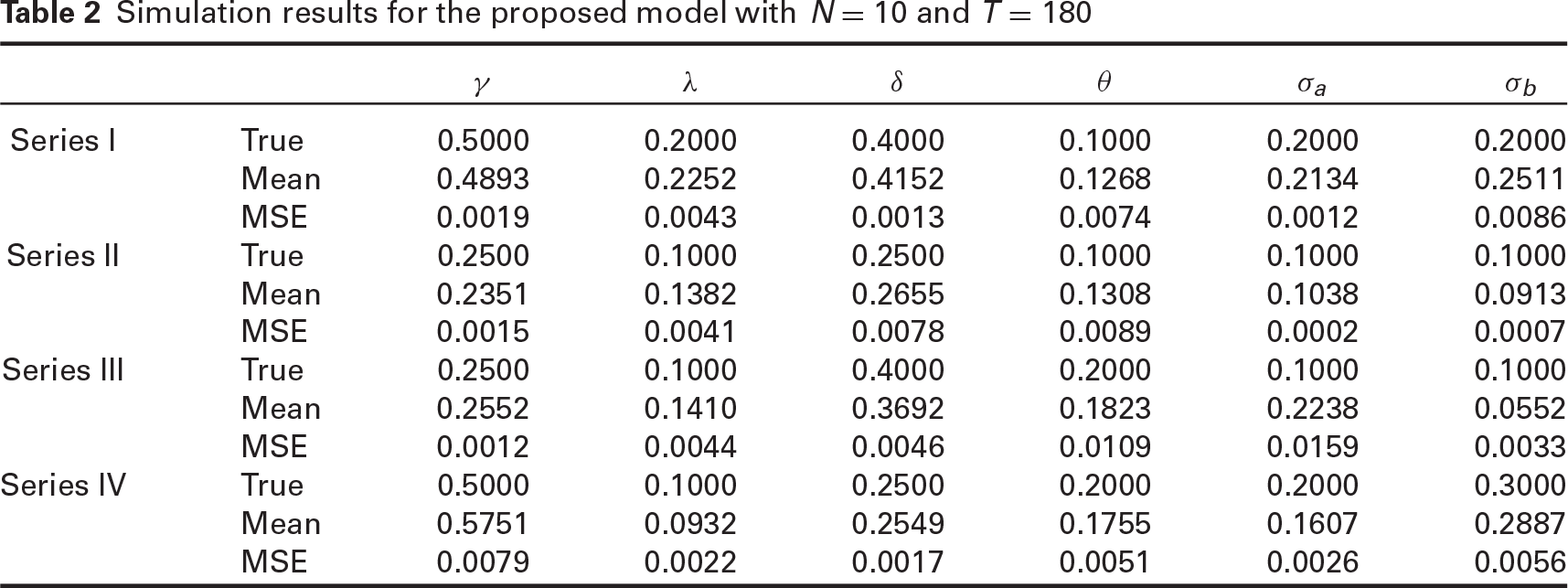
We first conduct a preliminary simulation study to investigate the Bayesian sensitivity analysis. Particularly, to evaluate the priors effect and hyperparameters choice on the posterior distribution, we examine a series of prior distributions, especially for variance components introduced by Gelman (2006), and study convergence by generating parallel chains. We also defined flat priors for all parameters respecting the already mentioned bounded supports. Simulation findings revealed that priors in Section 3 and flat priors produced almost the same estimation results, implying the model fitting was less sensitive to the choice of priors. For fixed hyperparameters in low-frequency equations, results of the simulated experiments were obtained by computing a series of means and mean-squared errors (MSEs) for all parameters of high-frequency equations. We organize several plans for simulations to investigate various properties of our proposed model:
Simulation results for the proposed model with different
and
Simulation results for the proposed model with different
and
Simulation results for the proposed model with
and
M1: The proposed model in Section 2.
M2: The proposed model with eliminating co-volatilities by assuming
M3: An extension of the univariate spline GARCH model proposed by Engle and Rangel (2008) to the multivariate case; for which,
M4: The Matrix-Diagonal model proposed by Ding and Engle (2001), with
M5: The heterogeneous multivariate GARCH model (Cermeño and Grier (2006)). Heterogeneity in
Existing MGARCH models have specific features, while some, such as M4 and M5, can not capture high- and low-frequency volatilities. The routine practice uses information criteria for models choice. First, let
Information criteria for fitted models
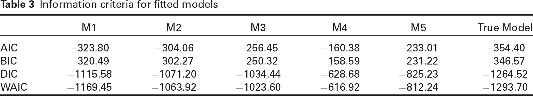
For each model, we ran Stan codes until successful convergence. Table 3 shows that the proposed model M1 performs satisfactorily compared to competing models since it has the least difference of criteria values with the true model. Notice that the data generating process was upon the contaminated normal distribution that involves outlying points. Thus, our results generally reveal that the fitted models involving cross-covariance, especially those accommodating more flexibility and variability through random effects, could deal with contaminated data, implying robustness to possible outlying points. The worst is M4 since it does not account for heterogeneity and volatility or co-volatility isolation.
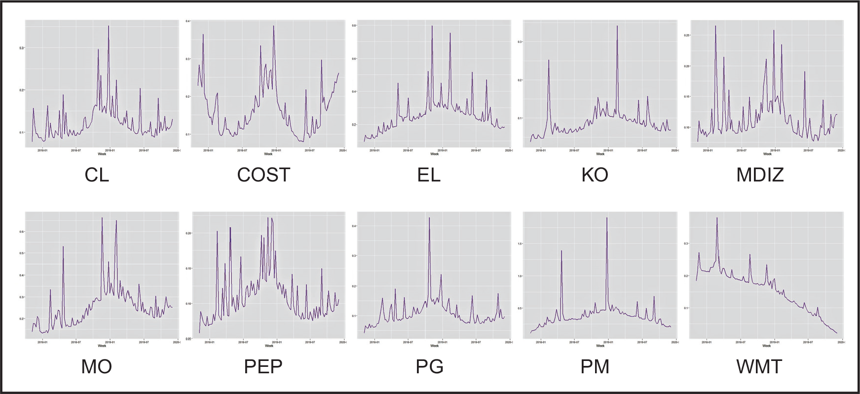
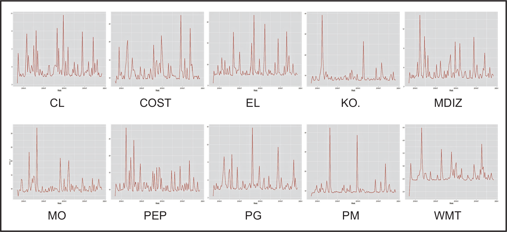
Stock market data analysis has often been desirable in economic and financial studies. As emphasized, the long-term and short-term changes in a stock price cause significant effects on other stocks and macroeconomic factors. Modern regression volatility models, such as widely used GARCH, are available to investigate the impact of such effects. This section analyses the weekly log-returns of the 10 top stock indices from the Consumer Staples sector. Our study contains Walmart (WMT), Procter and Gamble (PG), Coca-Cola (KO), Philip Morris International (PM), Altria Group (MO), Estee Lauder (EL) and Colgate-Palmolive (CL) from the New York Stock Exchange (NYSE), and PepsiCo (PEP), Costco (COST) and Mondelez International (MDLZ) from the National Association of Securities Dealers Automated Quotations exchange (NASDAQ). The data cover 110 weeks from 6 November, 2017 to 2 December, 2019, and is freely available on
Time-series plots for the log-returns of 10 stocks
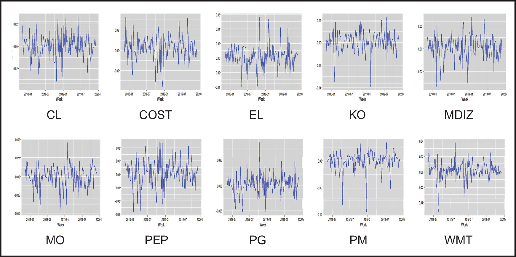
Time-series plots for the log-returns of 10 stocks
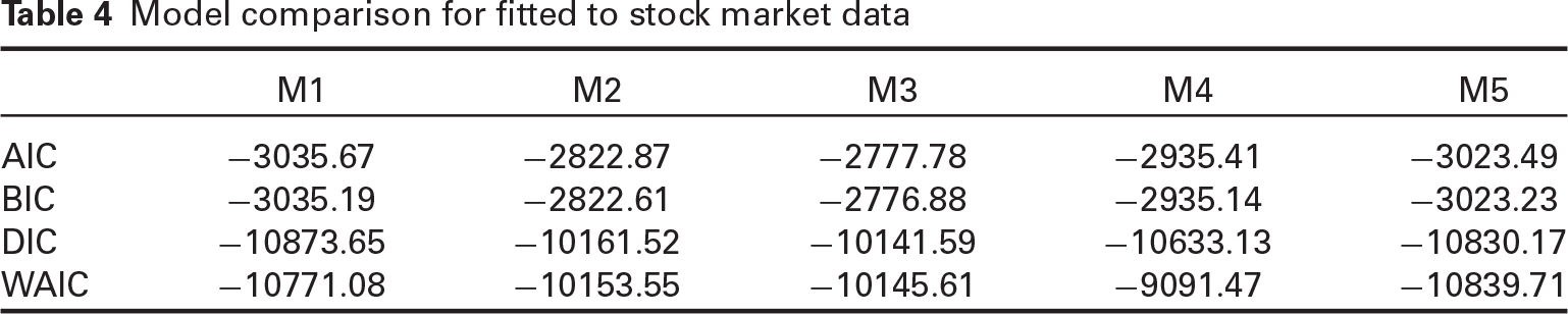
Now, we assess the proposed model performance in empirical applications compared to current models for cross-correlated financial data. It is instructive to signify model's ability to isolate high- and low-frequency volatilities. Estimation results, shown in Table 4, reveal that our model is the best fitting. Although the heterogeneous multivariate GARCH model fits fairly satisfactorily, it cannot isolate frequencies, unlike our model.
Model comparison for fitted to stock market data
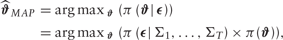
As mentioned in Section 3.3, the RStan library in R utilizes the HMC simulation approach. Stan provides the mode of posterior or the MAP estimate. The Newton-Raphson algorithm is the default optimization of Stan (Carpenter et al.(2017)). Also, by adopting non-informative priors, the MAP estimates are equivalent to the MLEs. Table 5 presents the estimation results for the given period.
Bayesian results, standard deviations, MLE and MAP estimates, and rhat values
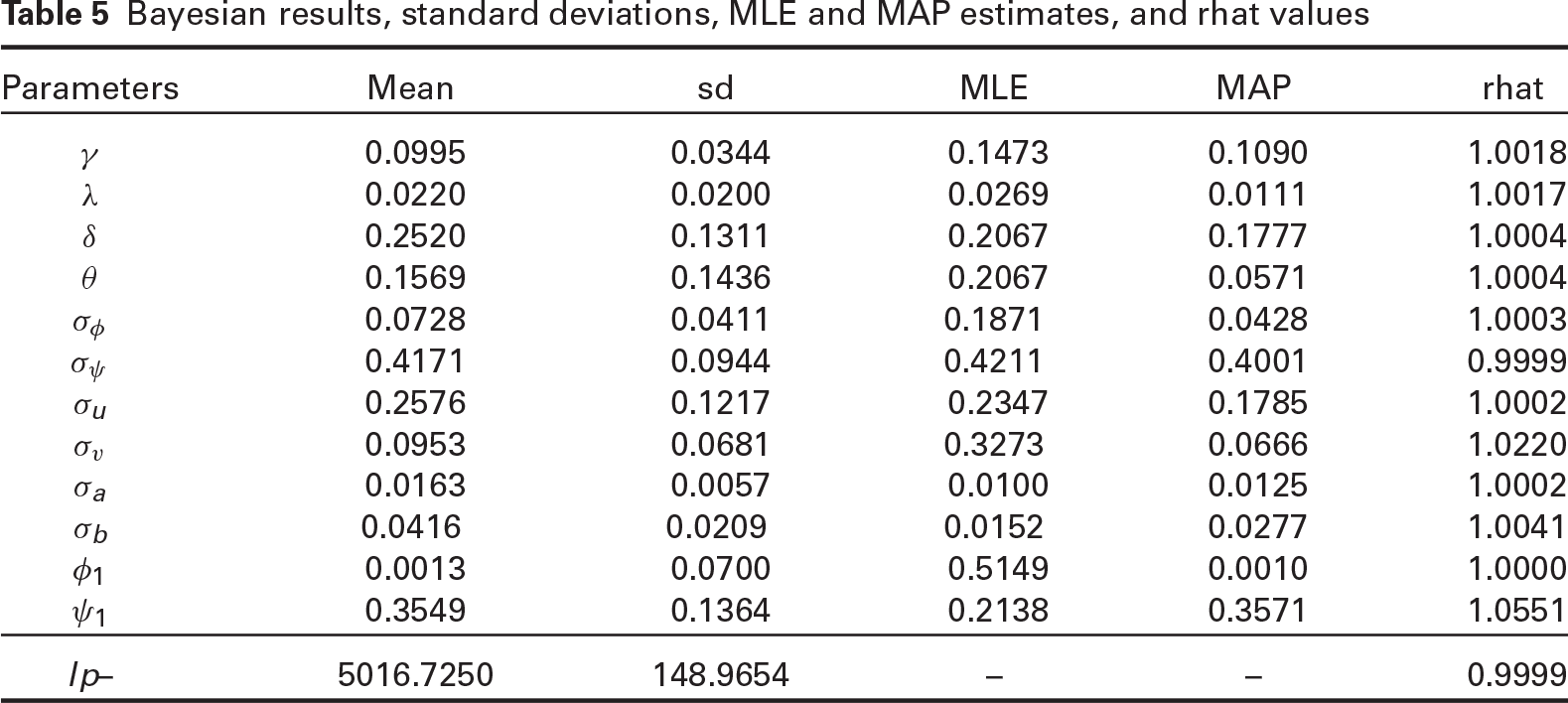
The random-effects
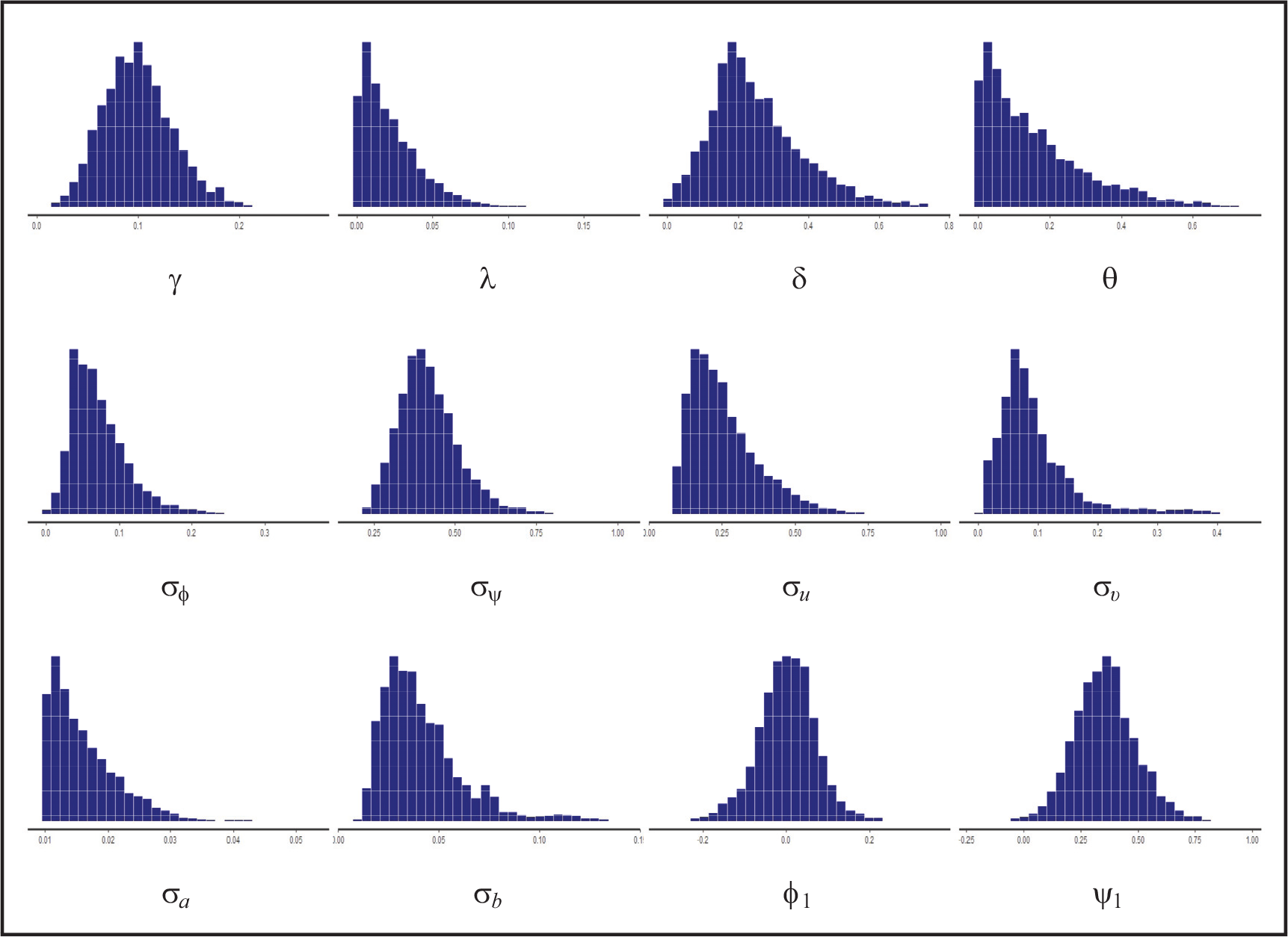
A convergence diagnostic in Stan is the rhat. It is close to one in Table 5, showing that all chains have converged to the same stationary distribution. Stan uses a more conservative version of rhat than its usual form in other packages, such as Coda (Plummer et al.(2006)). By default, it divides each chain in half to identify non-stationary chains (Gelman et al.(2013); Carpenter et al.(2017)). Trajectories of all parameters estimated over simulations and changes within a reasonable tolerance level (not shown here) showed a well-mixed chain. Figure 2 shows the posterior predictive histogram.
Predictive posterior histograms
The individual high-frequency volatility
Time-varying variance components for the log-return of 10 US stocks
High-frequency volatility in the log-return of 10 US stocks
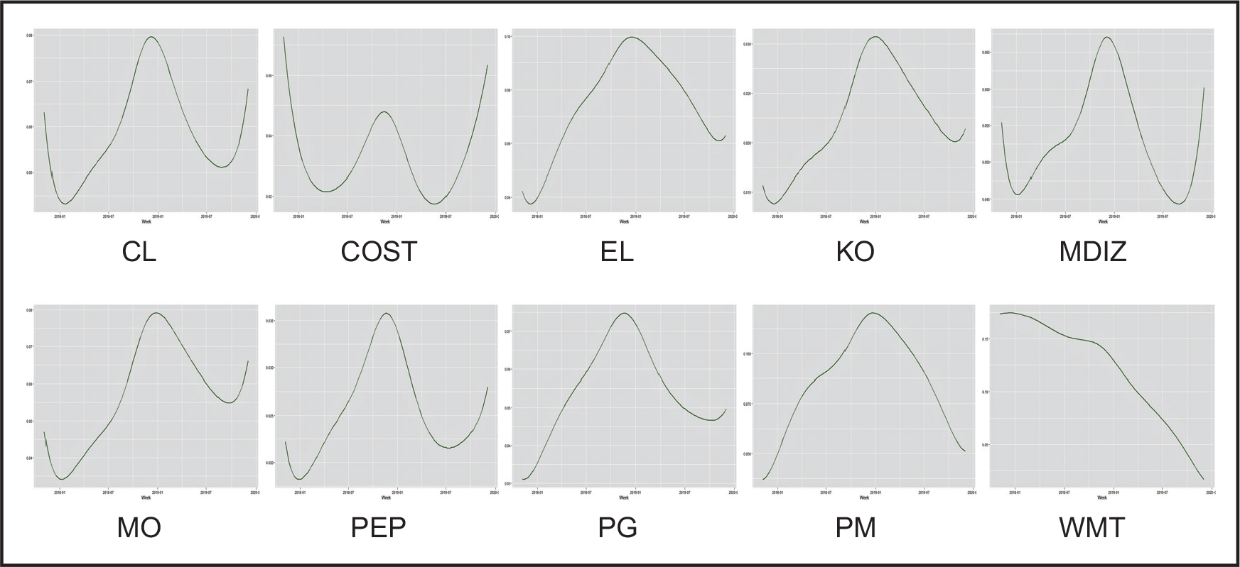
Low-frequency volatility in the log-return of 10 US stocks (
scaled up)
(A) Time-varying covariance and (B) Low-frequency co-volatility of the WMT and 9 other log-returns (
scaled up)
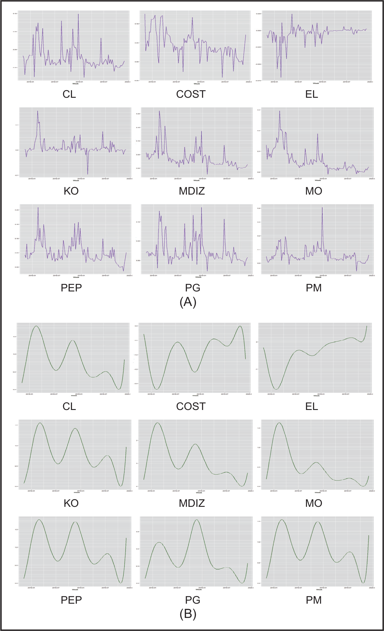
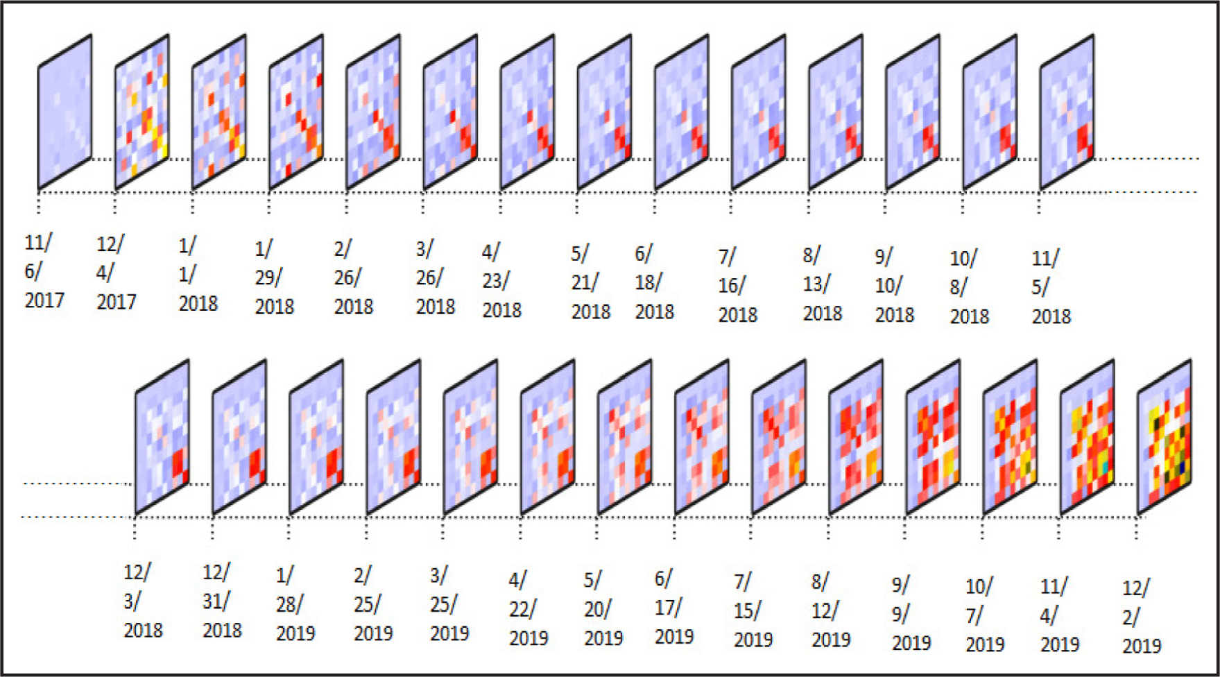
To study the co-volatility in the covariance equation, consider the WMT index as an example. Figure 6 illustrates the low-frequency co-volatility and the time-varying covariance for the log-return of Walmart's stock and the nine other stocks. Low-frequency plots display the smoothness of covariances patterns. Figures describe the long-term changes of the WMT when other stocks have presented. Short-term volatility immediately affects the log return, while long-term volatility plays a role in the decision for future trades. The covariance structure is more influenced by long-term than short-term changes for this dataset. As seen here, coefficients in the low-frequency model are significant, unlike in the high-frequency model. It means that the volatility in one stock has a long-term impact on other stocks. When unexpected changes in one stock immediately impact other stocks, there is higher economic instability in the financial markets. Figure 7 presents the temporal heatmap for the time-varying covariance matrix for some selected days over this period.
Temporal heatmap for the time-varying covariance matrix
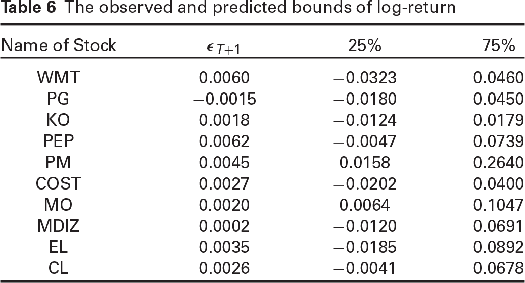
Forecasting volatility is particularly important for companies concerned with portfolio management, and brokers will trade stocks more confidently. There are various methods to estimate or predict volatility. The accurate estimate of a future market trend confirms the proposed model is appropriately fitted. To evaluate prediction accuracy, we first remove the vector observed at the time
The observed and predicted bounds of log-return
Heatmap of the predicted covariance matrix
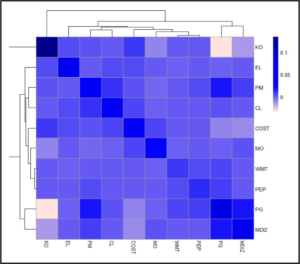
Moreover, the multivariate analysis can predict the cross-covariance of stocks involving their latent short- or long-run effects. Figure 8 displays a one-step-ahead forecast of the covariance matrix. Closer pairs of stocks indicate a higher covariance and darker colours over the heatmap. It graphically represents cross-dependence at time
The article introduced a flexible model for describing high- and low-frequency variations with novel data analysis methods. Specifically, we offered modelling strategies for cross-sectional time-series analysis with serially correlated innovation terms and cross-individual dependence. The related conditional variance and covariance components followed the spline-GARCH process. In particular, we proposed a non-parametric regression model of the penalized low-rank smoothing spline form to account for time trends in the variance and covariance equations. Our proposed strategy can provide flexible modelling on the low-frequency volatility in equity markets. The model can differentiate non-parametrically dynamic patterns of high- and low-frequencies of variance-covariance structural equations and incorporate economic features to predict stock market volatility based on the time-series evidence. Many financial and macroeconomic time-series data are often conditionally heteroscedasticity, meaning that traditional estimation methods produce inefficient estimates. To analyse such data, taking advantage of advanced numerical methods is required. The HMC sampler can estimate related variances and covariances components in the normal case using computational Bayes. Future studies aim to present flexible multivariate distributions to analyse such correlated data with skewed structures.
Supplementary materials
Supplementary materials for this article containing software codes are available from
Footnotes
Acknowledgments
We are grateful to the Editor and two anonymous referees for their constructive comments. We thank the Shiraz University Research Council for supporting this work.
Declaration of conflicting interests
The authors declared no potential conflicts of interest with respect to the research, authorship and/or publication of this article.
Funding
The authors disclosed receipt of the following financial support for the research, authorship and/or publication of this article: The authors acknowledge the Iran National Science Foundation for partial financial support (INSF 96012003).