Nonlinear discrete-time hazard models for women's entry into marriage

Abstract

We propose a hazard model for entry into marriage, based on a bell-shaped function to model the dependence on age. We demonstrate near-aliasing in an extension that estimates the support of the hazard and mitigate this via re-parameterization. Our proposed model parameterizes the maximum hazard and corresponding age, thereby facilitating more general models where these features depend on covariates. For data on women's marriages from the Living in Ireland Surveys 1994–2001, this approach captures a reduced propensity to marry over successive cohorts and an increasing delay in the timing of marriage with increasing education.

1 Introduction

Changes in family formation over recent decades have provided an interesting field of research for social scientists. In Western countries, there has been a rapid increase in the age at which people enter into marriage and start a family (Caldwell et al.(1988); Blossfeld (1995)). Women now postpone marriage and parenthood until they have completed their education and entered the labour market (Skirbekk et al.(2004)). The delay in family formation is thus partly explained by women's increased participation in education (Blossfeld and Jänichen (1992)).

The effects of factors such as educational attainment and labour force participation can be investigated to some extent by cross-sectional analyses. However, in order to relate women's choices to previous educational and career experiences, it is necessary to analyse life course data (Blossfeld and Huinink (1991)).

In this article, we model the transition from being unmarried to entering marriage using discrete-time survival analysis techniques. We present our approach through application to data from the Living in Ireland Surveys, which are described further in Section 2. Ireland is of particular interest because demographic changes have tended to occur later there than in other Western societies. Although we consider the timing of first marriage in this case, our approach could equally be applied to the timing of other events with similar characteristics, such as first pregnancy.

We define the survival time, $T$ , to be the number of calendar years an individual remains unmarried from the year in which they reach the minimum legal age of marriage. If $t\in \{0,1,2,...\}$ is the number of calendar years since reaching the minimum legal age, then the hazard of entry into marriage at time $t$ is defined as

$$h(t)=P(T=t|T\ge t).$$

(1.1)

Our aim is to develop models for this hazard and we initially work within the familiar proportional hazards framework. A discrete-time analogue of the proportional hazards model for an individual $i$ with covariates ${\mathbf{x}}_{\mathit{it}}$ may be formulated as

$$(h(t|{\mathbf{x}}_{\mathit{it}}))=(h_0(t))+{\mathbf{x}}_{\mathit{it}}^{\prime }\mathbf{\beta },$$

(1.2)

where $h_0(t)$ is the baseline hazard (Cox and Oakes (1984)). This model approximates the continuous-time proportional hazards model when the hazard is small (Yamaguchi (1991)). Using the logit link provides a direct interpretation in terms of the conditional odds of marriage.

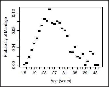
Applying the non-parametric baseline hazard model of Equation 1.2 to our motivating dataset gives the piecewise constant hazard function shown in Figure 1. This figure illustrates the non-monotonic dependence of the hazard on age that is typical for events such as entry into marriage. A disadvantage of the Cox proportional hazards model is that it requires a large number of parameters to be estimated, since the hazard is estimated separately for each year of age. It can be seen in Figure 1 that these estimates are increasingly susceptible to outliers with increasing age, as the number of unmarried women decreases.

Figure 1:

The fitted non-parametric discrete-time hazard model (Equation 1.2) for the Living in Ireland data

An alternative approach is to model the overall pattern of the baseline hazard using a parametric function, which will require far fewer parameters to be estimated. (Blossfeld and Huinink (1991)) propose the following parametric baseline,

$$(h_0(t))=c+{\beta }_l\text{log}({\mathit{age}}_{\mathit{it}}-15)+{\beta }_r\text{log}(45-{\mathit{age}}_{\mathit{it}})=\mathit{BH}({\mathit{age}}_{\mathit{it}}),\mathit{say},$$

(1.3)

which forms a bell-shaped curve. This model makes the assumption that non-zero hazard of entry into marriage only exists between the ages of 15 and 45. These endpoints correspond to the age range over which marriages were observed in the (Blossfeld and Huinink (1991)) study. While the left endpoint is clearly governed by the legal age of marriage (16 years old), the right endpoint is simply an artefact of the study design, since it corresponds to the final age of follow-up. The approach of (Blossfeld and Huinink (1991)) has been applied to a collection of other Western countries (Blossfeld (1995)), in which a common right endpoint was used in the baseline model, even for countries where marriages of women aged above this endpoint were observed (Oppenheimer et al.(1995); Pinnelli and De Rose (1995)).

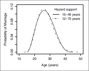
Although the exceptional cases of early or late marriages are of minor interest in a general study of trends in the timing of marriage, the determination of the endpoints in Equation 1.3 is important because they have an effect on the entire shape of the fitted model. For example, Figure 2 shows the curve obtained for the Living in Ireland data when Equation 1.3 is used to define the model, overlaid by the fitted curve for a model with the same parametric form, but with the support of the hazard being 12 to 75 years of age. It can be seen from this figure that the change in endpoints makes very little difference to the fitted hazard at ages less than 16 or greater than 45, but makes an appreciable difference over the range 24 to 44 years of age.

Figure 2:

The fitted linear discrete-time hazard model (Equation 1.3) for the Living in Ireland data: — support of the hazard fixed at 15–45 years; $·$ – $·$ support fixed at 12–75 years

Therefore it would be desirable to estimate the support of the baseline hazard as part of the model, allowing greater flexibility over the shape of the fitted model without adding an excessive number of parameters. An immediate extension of Equation 1.3 would give the nonlinear baseline

$$(h_0(t))=c+{\beta }_l\text{log}({\mathit{age}}_{\mathit{it}}-{\alpha }_l)+{\beta }_r\text{log}({\alpha }_r-{\mathit{age}}_{\mathit{it}}).$$

(1.4)

We shall demonstrate that this straightforward extension suffers from near-aliasing between the parameters, such that a change in one parameter can be compensated for by changes in the remaining parameters. We therefore propose an alternative parameterization, a re-expression of the same model in which the correlation between parameters is reduced. With this model, it is possible to test whether assumptions made about the endpoints are validated by the data. Furthermore, the parameters of the re-expressed model have a more useful interpretation than those in Equation 1.4. This allows us to consider a general class of informative models for the Living in Ireland data, in which there are interactions between the covariates and directly interpretable parameters of the baseline hazard. We shall show that such models capture important features of the data.

The remainder of the article is organized as follows. First we provide further details of our data from the Living in Ireland Surveys. Then in Section 3 we follow the approach of (Blossfeld and Huinink (1991)) to build a reference linear discrete-time hazard model for these data. In so doing, we contribute to the collection of studies that have followed the approach of (Blossfeld and Huinink (1991)) in (Blossfeld (1995)). In Section 4, we demonstrate the near-aliasing that occurs when Equation 1.4 is used as a baseline and go on to show the improvement that is offered by our proposed re-parameterization. We repeat the analysis of Section 3 with the new baseline and consider further improvements to the model. Finally, we discuss our findings in Section 5.

One of the authors of this article (DF) had the good fortune to work for a short time in Murray Aitkin's group at Lancaster in the early 1980s—for just enough time, in fact, to be inspired by Murray to do a PhD! Some of Murray Aitkin's well-known work in modelling survival data was done at around that time (e.g., Aitkin and Clayton (1980); Aitkin et al.(1983)) and it featured prominently also in the highly influential book Statistical Modelling in GLIM (Aitkin et al.(1989)). We hope that the work in the present article emulates in some small way Murray's inventive approach to analysing such data, through modelling that relates closely to the application at hand.

2 Data

The Living in Ireland Surveys were conducted between 1994 and 2001 by the Economic and Social Research Institute. Full details of the surveys are given in (Watson (2004)). Data was collected by yearly household interviews, providing information on individuals’ education, occupation and standard of living, as well as basic demographics.

We shall consider only a subset of the data here. In particular we restrict our attention to women who were members of the original sample of households and who were born between 1950 and 1975, giving five, five-year cohorts (1950–1954, 1955–1959, 1960–1964, 1965–1969 and 1970–1974) who by 2001 had passed the mean age at marriage for women in the full dataset. This selection allows us to consider recent trends in the propensity to marry, while giving sufficient data to estimate models reliably.

We consider marital status as simply married or unmarried, and focus our attention on a selection of other variables: the year and month of birth, the social class (usually based on the father: unskilled, semi-skilled manual, skilled manual, non-manual, low professional, high professional or missing), the highest level of education attained (no formal education/primary, lower secondary, upper secondary, Post-leaving Certificate, Institute of Technology qualification or University qualification) and the corresponding year of attainment.

We use the method of episode-splitting (see e.g., Powers and Xie (2008); Blossfeld et al.(2019)) to generate yearly pseudo-observations for each individual, from the year in which they became 16 up to the year in which they either married, became 45 or were lost to follow up. The observations are assumed to be made at the start of the calendar year, so that the age at time $t$ is taken to be

$$16-(\mathit{monb}-0.5)/12+t,$$

where $t\in \{0,1,\dots \}$ is the number of calendar years since that in which the woman became 16 and $\mathit{monb}\in 1,2,\dots ,12$ is the month of birth. Our final dataset comprised 31 009 records for 2 902 women.

3 Linear discrete-time hazard models

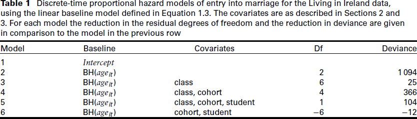
We conduct an initial analysis of the data using the discrete-time proportional hazards model (Equation 1.2) with the linear parametric baseline of Equation 1.3, which assumes that the support of the baseline hazard is known. We follow the analytic template of (Blossfeld (1995)): we start with the null model, add the baseline variables, then add social class, cohort and education variables in turn. The results are presented in Table 1.

Table 1

Discrete-time proportional hazard models of entry into marriage for the Living in Ireland data, using the linear baseline model defined in Equation 1.3. The covariates are as described in Sections 2 and 3. For each model the reduction in the residual degrees of freedom and the reduction in deviance are given in comparison to the model in the previous row

Model	Baseline	Covariates	Df	Deviance
1	Intercept
2	BH(age it )		2	1 094
3	BH(age it )	Class	6	25
4	BH(age it )	class, cohort	4	366
5	BH(age it )	class, cohort, student	1	104
6	BH(age it )	cohort, student	−6	−12

As in (Blossfeld (1995)), two education variables are considered. First, the effect of educational enrolment is modelled using a time-varying binary variable, ‘student’, which indicates whether the woman is in education or not at time $t$ . Second a dynamic measure of the level of education, ‘education’, is constructed based on the known final level of education and the typical age at which each level of education is obtained. Specifically, for women who have passed a certain level of education the measure is updated at the typical age of attainment with the typical number of years taken to reach that level of education (no formal education/primary: duration 8 years, attainment age 12 years old; lower secondary: 3 years/15 years old; upper secondary: 3 years/18 years old; post-leaving certificate: 1 year/19 years old; college qualification: 2 years/20 years old; university qualification: 3 years/21 years old). Consistent with the results for West German women presented by (Blossfeld and Huinink (1991)), we find that including this measure as a covariate does not significantly improve the model (results not shown). Once the student indicator is added to the model, the class factor can be dropped from the model without a significant increase in deviance (Table 1).

Thus the best model among those considered in Table 1 includes the baseline variables, the cohort factor and the student indicator. The coefficients of the baseline variables, ${\beta }_l$ and ${\beta }_r$ are estimated as 2.1 (s.e. 0.1) and 3.9 (s.e. 0.2) respectively, so the baseline hazard is right-skewed. Compared to the baseline cohort of women born in 1950–1954, the conditional odds of marriage for a woman of the same educational status are not significantly different in the 1955–1959 or 1960–1964 cohorts, but rapidly decrease through the later cohorts to 24% of the baseline conditional odds in the 1970–1974 cohort (95% confidence interval: 20%–30%). The conditional odds of marriage for a woman who is in education are 11% of those for a woman of the same cohort who is not in education (95% confidence interval: 6%–20%).

4 Nonlinear discrete-time hazard models

We now turn to a nonlinear discrete-time proportional hazard model in which the endpoints of the support of the baseline hazard are to be estimated from the data. We first fit the baseline model as defined in Equation 1.4 in R (R Core Team (2020)), using the gnm package for generalized nonlinear models (Turner and Firth (2020)). The endpoint parameters ${\alpha }_l$ and ${\alpha }_r$ need to be constrained to ensure that the log terms remain finite. To enforce the constraints ${\alpha }_l<{\mathit{age}}_{[\mathit{min}]}$ and ${\alpha }_r>{\mathit{age}}_{[\mathit{max}]}$ , where ${\mathit{age}}_{[\mathit{min}]}$ and ${\mathit{age}}_{[\mathit{max}]}$ are the minimum and maximum ages observed, we set

$$\begin{array}{cc}{\alpha }_l\hfill & ={\mathit{age}}_{[\mathit{min}]}-\text{exp}({\alpha }_l^{*})-{10}^{-5}\hfill \end{array}$$

(4.1)

$$\begin{array}{cc}\mathit{and}{\alpha }_r\hfill & ={\mathit{age}}_{[\mathit{max}]}+\text{exp}({\alpha }_r^{*})+{10}^{-5},\hfill \end{array}$$

(4.2)

then estimate ${\alpha }_l^{*}$ and ${\alpha }_r^{*}$ .

We observe that the standard errors of the resultant estimates are quite large, particularly for the intercept $c$ (estimate $-118.5$ , s.e. 201.6) and the second slope parameter ${\beta }_r$ (estimate 24.9, s.e. 38.6). Investigating further, we find that these parameters are almost perfectly negatively correlated and in fact all the parameters are highly correlated with each other (Table 2).

Table 2

Correlations between the estimated parameters of the baseline model as defined in Equation 1.4

	c	β l	α l	β r	α r
C	1.00000
β l	−0.92563	1.00000
α l	−0.80861	0.95844	1.00000
β r	−0.99999	0.92688	0.80989	1.00000
α r	−0.99833	0.90319	0.77910	0.99808	1.00000

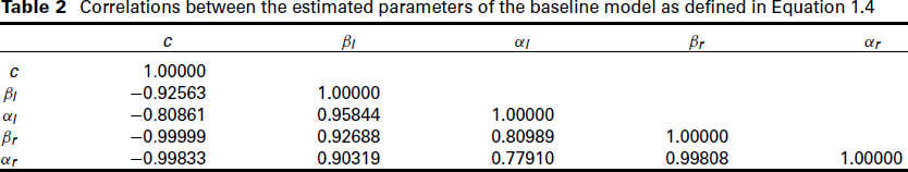
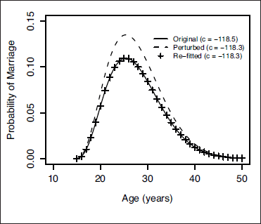
The effect of this near-aliasing can be demonstrated graphically using what we term ‘recoil plots’, an example of which is given in Figure 3. We plot the fitted model on the probability scale, then overlay the curve obtained by shifting one of the model parameters to a new value, and finally add the curve obtained when the parameters are re-estimated with the shifted parameter constrained to its new value. The near-aliasing is clearly apparent in Figure 3, since the re-fitted model coincides with the original model, that is, the other parameters compensate for the arbitrary shift. A similar plot is obtained for all the other parameters in the model.

Figure 3:

A ‘recoil plot’ for the intercept, $c$ , demonstrating the aliasing in the baseline model defined by Equation 1.4. Three hazard curves are shown: — the original fitted model where $c=-118.5$ ; –– the perturbed model with $c$ shifted to $-118.3$ and the other parameters left at their fitted values and ++ the re-fitted model with $c$ constrained to $-118.3$ and the other parameters re-estimated

Figure 4:

An illustrative hazard curve, showing how the parameters of the baseline model defined in Equation 4.2 relate to the features of the curve

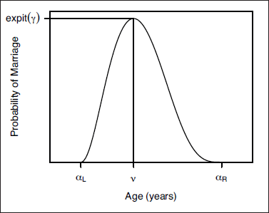
Although the near-aliasing does not prevent the use of Equation 1.4 as a model for the baseline hazard, it will make it harder to fit models including covariates. Therefore it makes sense to seek an alternative parameterization in which the parameters are less correlated and as far as possible have a direct interpretation in terms of the features of the hazard curve. We propose the following re-parameterization:

$$\begin{array}{cc}(h_0(t))\hfill & =\gamma -\delta \left\{(\nu -{\alpha }_l)\text{log}\left(\frac{\nu -{\alpha }_l}{{\mathit{age}}_{\mathit{it}}-{\alpha }_l}\right)\right\}\hfill \\ -\delta \left\{({\alpha }_r-\nu )\text{log}\left(\frac{{\alpha }_r-\nu }{{\alpha }_r-{\mathit{age}}_{\mathit{it}}}\right)\right\}\hfill \\ =\mathit{Bell}({\mathit{age}}_{\mathit{it}}).\hfill \end{array}$$

(4.3)

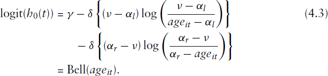
As illustrated in Figure 4, the parameters ${\alpha }_l$ and ${\alpha }_r$ correspond to the left and right endpoints as before, while $\nu$ gives the location of the peak hazard and $\gamma$ gives the maximum hazard on the logit scale. The fifth parameter, $\delta$ , does not have such a direct interpretation, but relates to the sharpness of the peak and can be loosely interpreted as the ‘fall off’ from the peak.

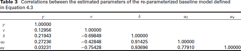
Re-fitting the baseline model with the new parameterization, we find that the correlation between parameters is much reduced (Table 3). In particular, the parameter $\gamma$ corresponding to the maximum hazard is only weakly correlated with the other parameters, so there should be little difficulty in allowing this parameter to depend on covariates or equivalently in adding covariates to the baseline hazard. The location of the peak, $\nu$ is moderately correlated with the other parameters so it will also be feasible to allow this parameter to depend on covariates. The remaining parameters are strongly correlated with each other, which is to be expected as they all influence the shape of the curve. However it might be reasonable to allow the fall off from the peak, $\delta$ , to depend on covariates.

Table 3

Correlations between the estimated parameters of the re-parameterized baseline model defined in Equation 4.3

	γ	ν	δ	αl	αr
γ	1.00000
ν	0.12956	1.00000
δ	0.21943	−0.69849	1.00000
α l	0.27236	−0.42848	0.91425	1.00000
α r	0.03231	−0.75428	0.93696	0.77910	1.00000

Figure 5:

Recoil plots for the parameters of the baseline model defined in Equation 4.2. In each case three hazard curves are shown: — the fitted model; –– the perturbed model with the parameter of interest shifted to a new value and the other parameters left at their fitted values, and ++ the re-fitted model with the parameter of interest constrained at its new value and the other parameters re-estimated

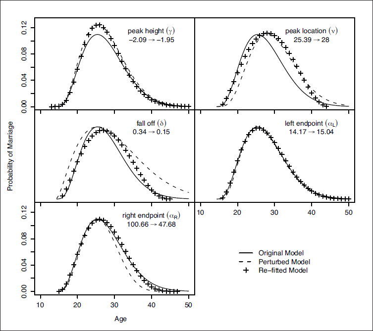
The correlations between the new parameters can again be illustrated by recoil plots (Figure 5). The plots for the parameters corresponding to peak height and peak location clearly show that a shift in either of these parameters cannot be compensated for by the remaining parameters. The plot for the fall off parameter $\delta$ shows moderate recoil towards the original model, whilst the plots for the endpoints show greater recoil but not so much that the re-fitted model is equivalent to the original model.

Using the new baseline, we repeat the analysis presented in Section 3, giving the results shown in Table 4. Compared to the linear baseline model (Model 2, Table 1) the nonlinear baseline model (Model 7, Table 4) reduces the residual deviance by about 20 at the expense of two degrees of freedom. A similar reduction in deviance is seen across the models and the estimated effect of the covariates on the hazard is little changed. Therefore the qualitative interpretation remains the same, but the residual deviance is significantly reduced by estimating the support of the hazard function from the data.

Table 4

Discrete-time proportional hazard models of entry into marriage for the Living in Ireland data, using the nonlinear baseline model defined in Equation 1.4. The covariates are as described in Sections 2 and 3. For each model the reduction in the residual degrees of freedom and the reduction in deviance are given in comparison to the model in the previous row

Model	Baseline	Covariates	Change in Df	Change in Deviance
1	Intercept
7	Bell(age it )		4	1 113
8	Bell(age it )	class	6	25
9	Bell(age it )	class, cohort	4	374
10	Bell(age it )	class, cohort, student	1	101
11	Bell(age it )	cohort, student	−6	−12

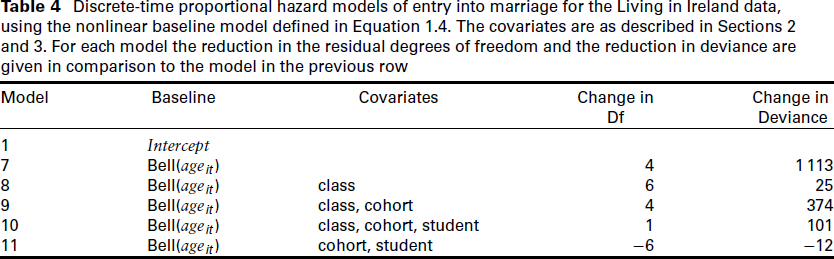
Moreover, we find that as the theoretically important variables are added to the model, the estimated endpoints of the support of the baseline hazard diverge from their constraints of $15\frac{1}{24}$ and $45\frac{23}{24}$ for the left and right endpoints respectively. In particular, the right endpoint in the final model (Model 11, Table 4) is estimated as 400.15 with a standard error of 3342.66. Given that this endpoint is so far from the data and indeed, in practical terms, may be regarded as representing the end of life, this finding suggests an alternative baseline in which the right endpoint is infinite. Letting ${\alpha }_r\to \infty$ in Equation 4.2 we obtain:

$$\mathit{Bell}({\mathit{age}}_{\mathit{it}}|{\alpha }_r=\infty )=\gamma -\delta \left\{(\nu -{\alpha }_l)\text{log}\left(\frac{\nu -{\alpha }_l}{{\mathit{age}}_{\mathit{it}}-{\alpha }_l}\right)+{\mathit{age}}_{\mathit{it}}-\nu \right\}.$$

(4.4)

Re-fitting Model 11 (Table 4) with an infinite right endpoint, the deviance is increased by only 0.01 on one degree of freedom, so there is no significant difference (Model 12, Table 5). However, setting the right endpoint at infinity allows the remaining parameters to be estimated with increased precision, for example the estimated ‘fall off’ changes from 0.47 (s.e. 0.25) to 0.50 (s.e. 0.07) and the left endpoint changes from 12.59 (s.e. 2.24) to 12.33 (s.e. 1.11). Under Model 12, the predicted hazard of entry into marriage during the coming year is zero (to 3 d.p.) for a 14-year-old regardless of educational status or cohort, whilst at the other end of the scale, the hazard becomes zero for all cohorts (to 3 d.p.) at age 51.

Table 5

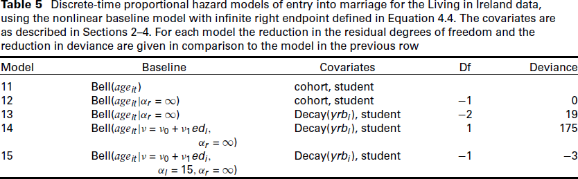
Discrete-time proportional hazard models of entry into marriage for the Living in Ireland data, using the nonlinear baseline model with infinite right endpoint defined in Equation 4.4. The covariates are as described in Sections 2–4. For each model the reduction in the residual degrees of freedom and the reduction in deviance are given in comparison to the model in the previous row

Model	Baseline	Covariates	Df	Deviance
11	Bell(age it )	cohort, student
12	Bell(age it |α r = ∞)	cohort, student	−1	0
13	Bell(age it |α r = ∞)	Decay(yrb i ), student	−2	19
14	Bell(age it |ν = ν0 + ν1 ed i , α r = ∞)	Decay(yrb i ), student	1	175
15	Bell(age it |ν = ν0 + ν1 ed i , α l = 15, α r = ∞)	Decay(yrb i ), student	−1	−3

So far we have restricted ourselves to the analysis strategy of Blossfeld and Huinink (Blossfeld and Huinink (1991)) to allow direct comparison with their approach. In so doing we have demonstrated that estimating the support of the hazard improves the fit of the model across the life course and gives sensible estimates of the (effective) endpoints based solely on the data. However, we now consider further improvements to the model and shall show that our proposed model for the baseline hazard has additional benefits in terms of capturing the features of the data.

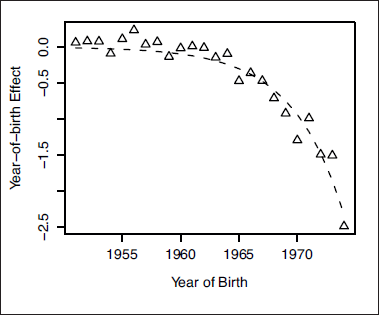
First we note that the cohort effects fitted by Model 12 have the pattern described in Section 3, that is, compared to the 1950–1954 cohort, the effects for the 1955–1959 and 1960–1964 cohorts are not significantly different from zero, whilst the effects for last two cohorts are increasingly negative. This suggests that the arbitrarily defined five-year cohort factor may not be the best device for modelling the underlying cohort effect. To investigate changes over the generations shown by the data, we fit an exploratory model in which the five-year cohort factor is replaced by a year-of-birth factor and plot the fitted effects (Figure 6). The pattern of the effects in Figure 6 shows that the hazard is much the same for women born between 1950 and 1964, after which there appears to be an exponential decay. This suggests that the underlying cohort effect may be more appropriately modelled by

$$\mathit{Decay}({\mathit{yrb}}_i)=\theta \text{exp}(\lambda ({\mathit{yrb}}_i-1950)),$$

(4.5)

where ${\mathit{yrb}}_i$ is the year of birth for individual $i$ . Fitting this curve directly to the year-of-birth effects seems to give a reasonable fit (Figure 6), so we include this nonlinear term in our model and drop the cohort factor. This reduces the deviance by 19 while increasing the residual degrees of freedom by 2 (Model 13, Table 5). A plot of the observed and fitted proportions for each year of age within each of the original five-year cohorts shows no systematic lack of fit (figure not shown).

Figure 6:

Estimated year-of-birth effects when the cohort factor in Model 12 is replaced by a year-of-birth factor. The effect for year-of-birth equal to 1950 is set to zero

We now consider whether the current model adequately describes the effect of education on the hazard. Figure 7 shows the observed and fitted proportions for each year of age, by highest level of education attained. The seven levels of education have been reduced to five, since the ‘sub-primary’ group and the ‘post-leaving certificate’ group were small in size and could be merged with the ‘primary’ and ‘institute of technology’ groups respectively as the patterns of observed proportions were not dissimilar. From Figure 7 we can see that the fitted model peaks too late for the lower education levels and too early for higher education levels.

Figure 7:

Fitted hazard curves for Model 13 (—), with a common peak location for all levels of education (common $\nu$ in the baseline model) and Model 14 (––), with a separate peak location for each level of education ( $\nu$ dependent on the dynamic measure of education level described in Section 3). The curves are laid over the observed proportion married for each year of age

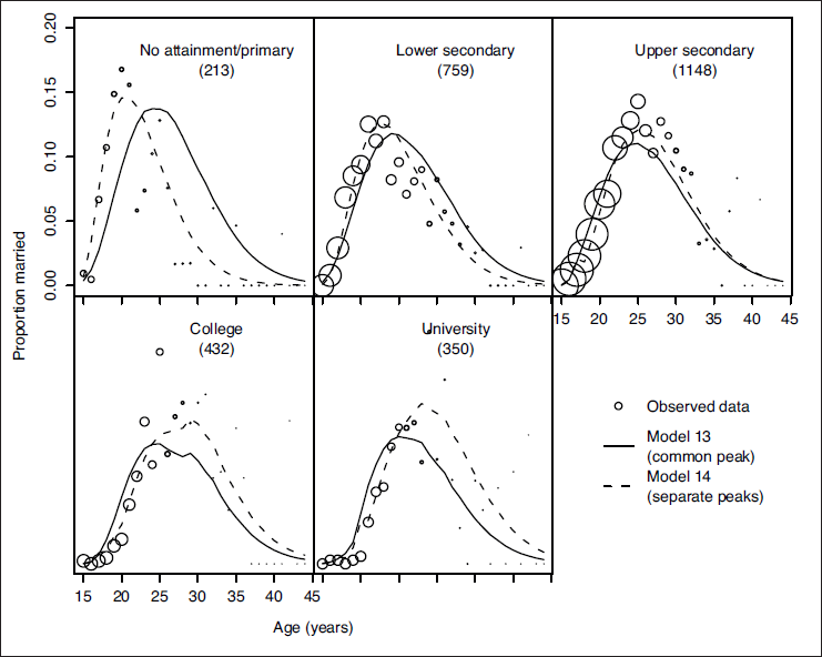
This suggests that a proportional hazards model, as often used in the analysis of timing of first marriage (e.g., in (Blossfeld and Huinink (1991)) and (Blossfeld (1995)), with Equation 1.3 as the baseline, in (Yabiku (2006)) and (Hank (2003)) with linear and quadratic effects of age as the baseline, or in (Katus et al.(2007)) and (Liefbroer and Corijn (1999)) using Cox's semi-parametric model), is not adequate here, since it is not the scale of the hazard that depends on education, but the location of the hazard. That is, the effect of further education is to delay the timing of marriage. Our proposed parameterization of the baseline hazard allows us to consider models that accommodate such trends in a natural way. In particular, the monotonic dependence of the peak location on education level shown in Figure 7 suggests an extension of the baseline model as follows,

$$\begin{array}{cc}\mathit{Bell}({\mathit{age}}_{\mathit{it}}|\nu \hfill & ={\nu }_0+{\nu }_1{\mathit{ed}}_i,{\alpha }_r=\infty )\hfill \\ \hfill & =\gamma -\delta \left\{({\nu }_0+{\nu }_1{\mathit{ed}}_i-{\alpha }_l)\text{log}\left(\frac{{\nu }_0+{\nu }_1{\mathit{ed}}_i-{\alpha }_l}{{\mathit{age}}_{\mathit{it}}-{\alpha }_l}\right)\right\}\hfill \\ \hfill & -\delta \left\{{\mathit{age}}_{\mathit{it}}-{\nu }_0-{\nu }_1{\mathit{ed}}_i\right\},\hfill \end{array}$$

(4.6)

where $\mathit{ed}$ is the dynamic measure of education level described in Section 3. Allowing the peak location to depend on the education level visually improves the fit (Figure 7) and significantly reduces the deviance (Model 14, Table 5).

Continuing to compare observed and fitted proportions over different sub-groups of the data does not reveal any notable lack of fit over age, class, year of birth, years since left education or calendar risk year. The left endpoint of the support of the hazard function is estimated by Model 14 as 14.5 years (s.e. 0.4). This suggests that the fit of the model would not be compromised by constraining the left endpoint to 15 years old, the expected value based on the legal age of marriage, and indeed we find that the deviance is not significantly increased by introducing this constraint (Model 16, Table 5).

Figure 8:

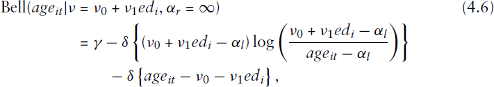
The fitted hazard curves under the final model (a) for women born in 1950, with different levels of education and (b) for women with no formal education/primary education, born in different years

Thus we come to our final model for the Living in Ireland data, the features of which can be shown by plots of the fitted hazard for different education levels and the same year of birth (Figure 8a) and for a selection of different years of birth assuming the same education level (Figure 8b). Considering first the effect of education (Figure 8a), the model incorporates the well-recognized heavy reduction in the hazard of entry into marriage while women are in education (conditional odds of marriage reduced by 84%, 95% confidence interval: 71%–91%), but also incorporates the delaying effect of education (peak hazard varies from 20.86 years (s.e. 0.22) for the group with no formal education to 27.44 years (s.e. 0.27) for university graduates). With regard to the cohort effect (Figure 8b), the peak hazard of entry into marriage for a woman born in 1950 is 0.17 (s.e. 0.05), dropping slightly to 0.15 (s.e. 0.03) for a woman born in 1960, but dropping down to 0.07 (s.e. 0.06) for a woman born in 1970. Clearly this model is inappropriate for predicting the hazard of marriage for women born after 1974 (the last year included in the analysis) as the peak hazard would soon be near-zero. A logistic term of the form

$$\frac{\theta }{1+\text{exp}(\lambda (\mu -({\mathit{yrb}}_i-1950)))}$$

(4.7)

may be more appropriate in this case, but it did not significantly improve the fit for our data.

Although it is convenient to model the hazard of entry into marriage, the primary outcome is the frequency distribution of marriages over the life course. We can translate the fitted probabilities from our final model into a frequency distribution of marriages simply by multiplying the probabilities by the number of women observed in the corresponding sub-categories. For example, Figure 9 (a) to (f) shows the observed and predicted frequency distributions for women born in 1950, 1960 and 1970. To compute the predicted frequencies, it is assumed that the initial numbers of women in each education level are as observed for that year of birth and that women then move into higher education levels in the same proportions as in the observed data for that cohort. In addition, it is assumed that the proportion of dropout is the same as observed from one age to the next. Comparing the observed and predicted frequencies in Figure 9 we see that the model captures well the overall shape of the distribution, the shift in location over the cohorts and the drop in scale over the cohorts.

Figure 9:

Observed and predicted marriages for women born in 1950, 1960 and 1970, subdivided by education $·$ university, $·$ institute of technology, $·$ post-leaving certificate, $·$ upper secondary, $·$ lower secondary $·$ no attainment/primary. Predictions are based on the initial numbers of women observed in each education level for the given year of birth and assume women move into higher education levels in the same proportions as they do in the observed data for that cohort. Bar plots (d) to (f) show the predicted number of marriages under the final model and bar plot (g) also predicts from the final model, but using 1950 as the year of birth rather than the true year of birth for the observed data, which is 1970

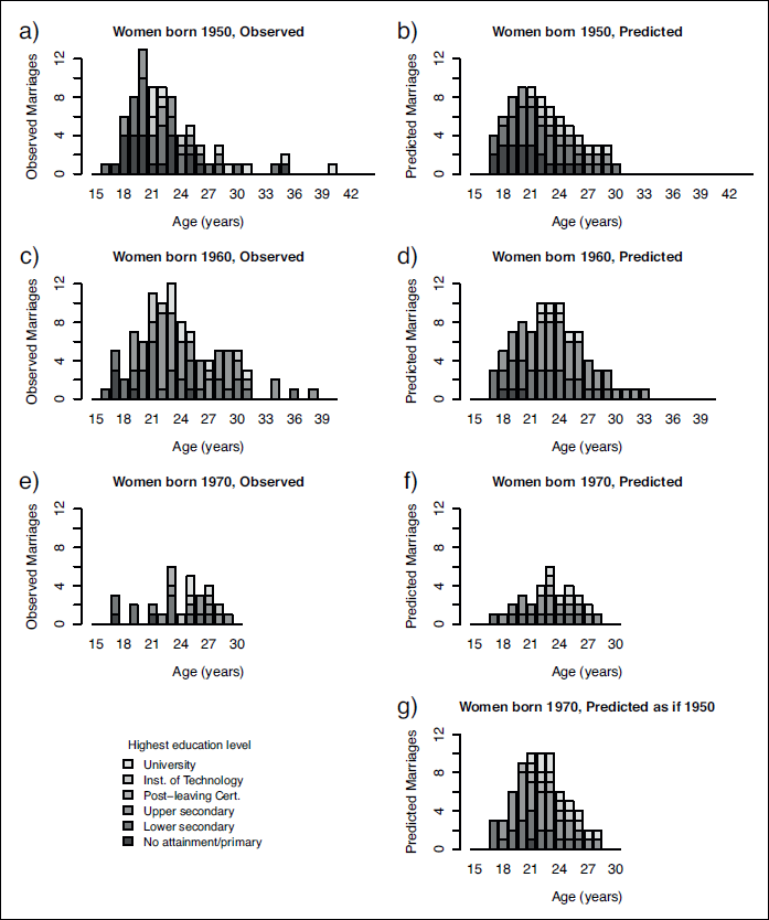
If we did not allow for a cohort effect, that is, if we assumed that the hazard of entry into marriage could be explained by education level and status alone, then we would still observe differences between the cohorts because of the increasing level of education over time. We illustrate this in Figure 9 (g) by predicting the distribution of marriages for women born in 1970, assuming that the hazard of marriage is the same as for women born in 1950, given the education level. The predicted distribution has its peak in roughly the same place as the observed distribution and the pattern over the education levels is similar, but we see that the predicted frequencies are much higher than those observed. Thus, the observed cohort effect cannot be explained purely by changes in education over time; there is an additional change in scale that affects all education levels.

5 Discussion

We have shown that it is not necessary to restrict the support of the hazard function to the age range represented in the sample and that doing so can significantly impair the fit of the model overall. Treating the right endpoint as a parameter allowed us to test the hypothesis of an infinite right endpoint, leading to the conclusion that the hazard of entry into marriage never completely disappears, but nevertheless is near zero at 45 years old, the endpoint that would have been used by the (Blossfeld and Huinink (1991)) approach. In our final model we found that the left endpoint was not significantly different from 15 years old, the age suggested by the legal constraints. Some of our earlier models suggested that the left endpoint was marginally, but significantly lower than 15. Such a result would also be plausible, implying not that there is an appreciable hazard of marriage under the legal age, but rather a slower increase in the hazard once the legal age is reached.

We have illustrated that a natural extension of a linear model to a nonlinear model can result in near-aliasing of the parameters and that this problem can be overcome through re-parameterization. In addition to estimating the support of the hazard function from the data, our proposed model has the benefit of more interpretable parameters, allowing investigation of the effect of covariates on both the location and scale of the maximum hazard. These features of the hazard curve are both the most interesting from a substantive point of view (Raymo (2003)) and the ones on which there is the most information in the data, so there is a good basis for such investigation. Consideration of the correlations between the parameters of the proposed baseline hazard suggests it may also be reasonable to allow the shape of the hazard to depend on parameters via the fall-off parameter, which may improve fit but could be harder to interpret.

Consistent with previous analyses following the approach of (Blossfeld and Huinink (1991)) (Blossfeld (1995); Blossfeld and Jänichen (1992)) we found that the scale of the hazard was markedly reduced while women were in education. However, the ability to allow the peak location parameter to depend on a dynamic measure of years spent in education also enabled us to show the delaying effect of education: women who spend longer in education postpone marriage until later. This finding is in line with the conclusions of Blossfeld and colleagues, but cannot be incorporated into the proportional hazards model proposed by (Blossfeld and Huinink (1991)).

In addition to the effect of education level, we observed an interesting trend over the different cohorts in the Living in Ireland study. For the early cohorts, women born between 1950 and 1964, we found no significant cohort effect. However, for women born after this we observed a sharp decline in the rate of marriage. We incorporated this effect into our model by using a nonlinear term based on the year of birth. This model would imply a decline in the propensity to marry from one generation to the next. An alternative explanation for the observed effect is that the propensity to marry is decreasing for all generations over time. In the context of studying fertility (Ní Bhrolcháin (1992)) argues that many of the relevant factors, such as the rising autonomy of women and rising secularism, are period- rather than cohort-specific. (Rodgers and Thornton (1985)) conclude that most of the trends in USA marriage rates over the first two-thirds of the twentieth century can be explained by period effects. However (Ní Bhrolcháin (1992)) also notes that ideational change may be cohort-specific, so our results highlight a need for further investigation of this issue in the context of marriage.

Bell-shaped hazard curves are observed for many social processes (Brüederl and Diekmann (1995)) and there have been a number of approaches used to model this type of hazard function. One simple approach is to include linear and quadratic effects of age in the predictor (e.g Yabiku (2006); Hank (2003); Gaughan (2002)). However this approach does not allow for the asymmetry that is often observed in the shape of the hazard. (Aalen (1992)) argues that the bell-shaped pattern may be explained by a frailty model, that is, the hazard curve for each individual need not be bell-shaped, but the hazard at the population level may show an initial increase and then decrease as the more susceptible individuals succumb to the event in question. However, while there may well be a heterogeneity effect that should be taken into account, we are interested here in the hazard for individual women and the factors affecting this hazard. The contribution of (Aalen (1992)), which in the illustrative analysis of marriage rates assumes a simple Weibull hazard for all women, does not help us in this respect.

The generalizations of the log-logistic model proposed by (Brüederl and Diekmann (1995)) are more in line with our approach. Their model has parameters for the timing, height and shape of the hazard function covering a wide variety of bell-shaped patterns as well as monotonic patterns. There are no parameters for the support of the hazard function — the left endpoint is fixed and the right endpoint is infinite — so inference can not be conducted on these aspects of the hazard curve. Moreover the timing and shape parameters have different effects compared to our peak location and fall off parameters. The timing parameter of (Brüederl and Diekmann (1995)) scales the time axis, changing both the location of the maximum hazard and the peakedness of the curve; while their shape parameter changes all aspects of the shape including the peak location and height. Therefore the two models will describe the effect of covariates on peak height in a similar way, but the overall shape and the effect of covariates on location will be described differently and either model may be more appropriate than the other in a given setting.

A parallel approach to modelling the hazard function is to model the probability density of marrying at a given age, which has a similar bell shape. The Coale–McNeil model (Coale and McNeil (1972)) is widely used in this context. (Kaneko (2003)) proposed a re-parameterization of the Coale–McNeil model in which one of the parameters corresponds to the location of the maximum probability, enabling models to be formulated in which the location depends on covariates such as education. The remaining parameters are described as ‘shape’ and ‘scale’ parameters, however both parameters affect all aspects of the density, including the maximum probability, the symmetry and the effective support of the function. Therefore it does not make sense to allow these parameters to depend on covariates and as such the model cannot capture effects such as the dependence of scale on educational status.

The parametric form of our model does impose some restrictions on the shape of the hazard curve, which means that the model does not always fully capture the pattern of the data. As discussed in Section 1, the Cox discrete proportional hazards model provides a simple alternative. The disadvantages of this approach are that several more parameters must be estimated, local features are over-emphasized and covariate interactions with the key features of the hazard curve can only be investigated by proxy. We believe that our proposed model strikes a useful balance between flexibility and interpretability.

In this article, we have assumed that all women are at risk of entering marriage during their lifetime. Of course a certain proportion of women will never marry and we could consider allowing for this in the model. The possibility of an infinite lifetime is naturally incorporated into the frailty model proposed by (Aalen (1992)) as an individual hazard of zero, while (Brüederl and Diekmann (1995)) propose a ‘mover-stayer’ model, explicitly estimating the proportion that never marry. Neither of these approaches is compatible with our model for the hazard function. However, it would be possible to extend the model to a competing risks model by allowing a multinomial response (Berrington and Diamond (2000)). In particular, allowing for cohabitation would account for the majority of women never married so that it becomes unnecessary to model this group separately.