
Abstract
In this article, we propose a longitudinal multivariate model for binary and ordinal outcomes to describe the dynamic relationship among firm defaults and credit ratings from various raters. The latent probability of default is modelled as a dynamic process which contains additive firm-specific effects, a latent systematic factor representing the business cycle and idiosyncratic observed and unobserved factors. The joint set-up also facilitates the estimation of a bias for each rater which captures changes in the rating standards of the rating agencies. Bayesian estimation techniques are employed to estimate the parameters of interest. Several models are compared based on their out-of-sample prediction ability and we find that the proposed model outperforms simpler specifications. The joint framework is illustrated on a sample of publicly traded US corporates which are rated by at least one of the credit rating agencies S&P, Moody's and Fitch during the period 1995–2014.
Keywords
Introduction
The last decades have witnessed an increased interest from practitioners in the financial industry, researchers and regulators alike in developing tools for appropriately measuring and modelling credit risk as well as developing and amending regulations which limit and monitor such risks. In this context, credit risk assessment typically relies on statistical models based on a historical database of defaults together with debtor-specific and market variables or on credit ratings which are forward-looking opinions of a debtor's creditworthiness and are assigned by external credit rating agencies (CRAs). This approach is also reflected in the regulations introduced in the Basel Accords I and II (Basel Committee on Banking Supervision (2004); Basel Committee on Banking Supervision (2011)). For example, under Pillar I of Basel II financial intermediaries can develop their own default prediction models, which, in case the history of defaults is limited and portfolio coverage is satisfactory, can be enhanced or replaced by models using external rating information. However, clear guidelines on how to integrate all available information sources into a proper modelling framework are scarce. More recently, the need of such an integrated approach has been stressed by both academia (e.g., Hilscher and Wilson (2017); Hirk et al., (2020)) and regulators with the IFRS 9 accounting standard issued by the International Accounting Standards Board (IASB (2014)) requiring banks to build provisions based on forward-looking expected loss models by considering ‘all reasonable and supportable information, including forward-looking measures’.
In this article, we extend the work of Hirk et al., (2020) and propose a framework for modelling defaults and credit ratings from Standard and Poor's (S&P), Moody's and Fitch in a multivariate ordinal model, where the latent credit quality is modelled as a dynamic process. The dynamic modelling of credit risk allows for dependencies in the cross-section and over time to be accounted for by typically making a distinction between systematic and idiosyncratic risk, where the systematic risk relates to the relationship between credit risk and a business factor and is of prime importance in portfolio credit risk modelling (see Vasicek (2002); Koopman and Lucas (2005); McNeil and Wendin (2007); Betz et al., (2018)). We therefore build a longitudinal model of binary default events and ratings on an ordinal scale where a common latent variable which is a measure of credit quality is underlying the observations. In particular, we model the conditional distribution of these responses given a set of financial covariates known to be relevant for credit risk modelling by assuming that the latent variable corresponding to the credit quality, referred to in this article as a ‘probability of default (PD) score’, depends on unobserved firm-specific effects, and on a systematic as well as an idiosyncratic factor which both have an auto-regressive structure of order one. This approach allows us to disentangle differences in firms’ credit quality due to idiosyncratic causes from the effects due to business conditions. In modelling the credit ratings we also consider several characteristics of the ratings market. First, CRAs claim to provide a forward-looking long-term measure of credit quality by employing a so-called ‘through-the-cycle’ (TTC) approach to ensure that their ratings are stable over the business cycle (as opposed to a ‘point-in-time’ (PIT) approach, which measures credit quality at a given point in time). Second, we do not disregard the criticism of the three big CRAs for their inability to assess risk accurately (e.g., Becker and Milbourn (2011); Bolton et al., (2012); Bar-Isaac and Shapiro (2013); Kashyap and Kovrijnykh (2016)) and, from the modelling perspective, we assume the ratings to be noisy observations of the underlying PD score by assuming a rater ‘bias’ for each of the CRAs which depends on covariates and has a time-varying component common to all the CRAs which captures yearly shifts in the rating standards of the rating agencies. Here, we resort to Bayesian estimation techniques implemented in the open-source software
Over the last decade, joint modelling frameworks for credit risk measures have become more popular but it is still common practice in both industry and academia to model defaults and credit ratings separately. Statistical binary response (typically logit) models are often employed for predicting defaults (among the most prominent articles in the finance literature, for example Shumway (2001); Campbell et al., (2008); Tian et al., (2015)), while static ordinal or linear regression is used in modelling the credit ratings (e.g., Alp (2013); Baghai et al., (2014)). Ordered regression models with a dynamic specification have also been employed for modelling rating transitions (e.g., Malik and Thomas (2012); Creal et al., (2014)). Several articles have jointly investigated different credit risk measures, including credit ratings from possibly various raters for the purpose of credit risk measurement. For example, (Hornik et al., (2010)) propose a static parametric framework based on the existence of contemporaneous PD estimates for the same obligor provided by different rating sources for estimating consensus ratings as well as validate the different rating sources by analyzing the mean/variance structure of the rating errors. (Grün et al., (2013)) extend the analysis to a dynamic model and analyze a panel of ratings from the three big CRAs by first transforming ratings to PD estimates by using observed default rates. (Creal et al., (2014)) build a multivariate dynamic factor model for signal extraction and forecasting of macro, credit, and loss given default risk conditions in the US. (Hilscher and Wilson (2017)) provide an analysis of both ratings and defaults (even though not in a joint statistical model) where they investigate whether the measures have different information content. They conclude that, while the credit ratings are poor measures of raw default probabilities, they are strongly related to systematic risk. (Hirk et al., (2018)) build a joint ordinal model for the ratings from the big three CRAs while (Hirk et al., (2020)) propose a static framework for jointly modelling defaults and ratings using the class of multivariate ordinal regression models and show improved results in terms of default prediction conditional on the observed ratings.
The article is organized as follows: The joint modelling framework is introduced in Section 2 and details regarding the estimation and prior specifications are presented in Section 3. Section 4 introduces the data set used in the analysis and presents the results while Section 5 concludes the article.
Modelling framework
General set-up
Suppose that for each firm
The one-year probability of default of firm
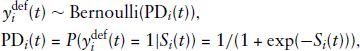
where
For the credit ratings, we employ an ordinal regression model using the cumulative link approach by treating the ratings observed for the

where
By allowing rater-specific thresholds we are able to capture the heterogeneity in the rating scale and methodology of the different CRAs. [The raters employ different coding for the rating classes: S&P and Fitch employ a rating scale with eight main non-default rating categories AAA, AA, A, BBB, BB, B, CCC, CC while Moody's scale is Aaa, Aa, A, Baa, Ba, B, Caa, Ca. Moreover, the CRAs claim to use different credit risk measures in their assessments: Moody's relies on loss given default while S&P and Fitch measure the relative likelihood of default.] Furthermore, in this application one may think of the term
Dynamic specification of the latent PD score
The basic framework underlying dynamic models of credit risk also adopted by regulators (see, e.g., the methodology underlying the CreditMetrics

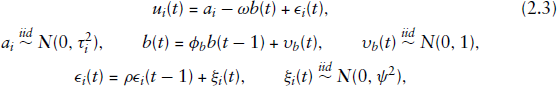
The rater bias specification proposed in this article is given by:

The rater factor
Bayesian inference
Several methods can be considered for the estimation of the proposed model, which contains effects at different levels of hierarchy. The non-nested firm and time effects, however, restrict the techniques which can be employed, as the estimation of ordinal models with non-nested effects is cumbersome due to the necessity to compute high-dimensional integrals. The maximum likelihood approach using the EM algorithm can be employed (e.g., Cagnone et al., (2009) employ the EM algorithm in estimating a multivariate ordinal model with item and time-specific random effects). (McCulloch (1994)) proposed the inclusion of a Metropolis Hastings step in the E-step of the EM algorithm so that the required expectation can be approximated by the average of Monte Carlo samples from the target distribution (approach used by, e.g., Xie et al., (2013) in a two-level model). (Bellio and Varin (2005)) tackle the dimensionality issue by maximizing the product of the pairwise marginal likelihoods and estimate the parameters of a two-level generalized linear mixed model (GLMM) with crossed random effects. The Bayesian framework is an attractive alternative for multi-level models with (crossed) effects at different levels of hierarchy. Through the specification of a prior distribution, Bayesian estimates of the effects can be obtained even in cases where there are few data points per group Moreover, the growing number of available open software tools for performing Bayesian inference make the implementation and estimation of such models more accessible.
Posterior
The posterior, which is proportional to the product of the likelihood of the four responses and the prior densities on all unobservables (i.e., parameters and latent quantities), is the object of interest in the analysis and inference relies on samples drawn from this posterior distribution. Samples from the posterior are drawn by using the package rstan (Stan Development Team (2019)) for R (R Core Team (2020)), which is an interface to the open-source software
Conditional on the latent PD scores
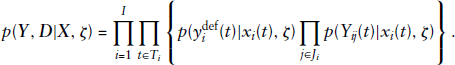
The term of the likelihood corresponding to the default indicator is given by the Bernoulli probability mass function
Priors are set on all model parameters. We find the results to be insensitive to the prior specified on the coefficients in the multivariate ordinal regression, which is to be expected given that the covariates were pre-selected based on their relevance in the existing literature. For the coefficients
Model evaluation and out-of-time prediction
In order to evaluate the performance of the model in terms of out-of-sample prediction, we use two approaches. First, we employ approximate leave-one-out (LOO) cross-validation methods (as proposed in Vehtari et al., (2017)). Second, we perform a
Assume we fit model

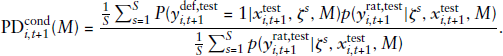
In addition to the joint posterior predictive densities, for the application case it is also relevant to assess whether adding the information about the ratings at the end of each year conditionally improves the prediction of the default component (see, e.g., Hirk et al., (2020)). Hence, for a future default observation
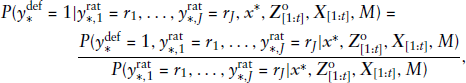
The predictive performance of
Given that the integrals such as the one in (3.1) cannot be solved analytically, they may, however, be approximated through Monte Carlo integration. Assuming the posterior distribution the posterior mean conditional default probability for firm
In this section, we introduce the dataset used in the analysis and proceed with a discussion of the results obtained from the proposed dynamic framework as well a with comparison to benchmark models in terms of the predictive performance.
Throughout the analysis, the hyper-parameters for the dynamic specification are kept constant. We set
Data
The empirical analysis is performed on a dataset containing credit ratings from S&P, Moody's and Fitch, default data and firm-level information for a sample of publicly traded and rated US corporates, excluding financial and utilities companies over the period 1995–2014. Long-term issuer credit ratings of S&P were downloaded by the S&P Capital IQ's COMPUSTAT North America Ratings file. The ratings from Moody's and Fitch were purchased by the research institution directly from the CRAs. Data on corporate defaults and bankruptcies were obtained from the UCLA-LoPucki Bankruptcy Research Database and the Mergent issuer default file. Firm-level data was downloaded from the merged COMPUSTAT/CRSP database.
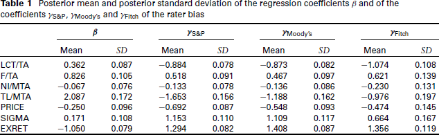
We perform the analysis on a calendar year basis and match the latest available firm-level information with all available end-of-year ratings. The default indicator is set to one whenever we observe a bankruptcy filing under Chapter 7 (liquidation) or Chapter 11 (reorganization) of the US bankruptcy code or if a default rating [Default ratings assigned by a CRA include in distressed exchanges or missed interest payments addition to bankruptcy filings.] is assigned by at least one CRA in the year following the rating observations. In all other instances, the default indicator is set to zero, including cases where the firm disappears from the dataset for some reason other than bankruptcy such as acquisition, delisting or if no longer rated. The firm-level information is used to construct covariates which have been identified as significant predictors of credit quality in the literature. In our analysis, we rely on the work of (Tian et al., (2015)), who employ model selection techniques to identify factors relevant for bankruptcy prediction: current liabilities/total assets (LCT/TA), total debt/total assets (F/TA), net income over market value of total assets (NI/MTA), annualized standard deviation of stock returns over a three month period (SIGMA), the logarithm of the end-of-year stock price, whereas the stock price is capped at USD 15 (PRICE) and gross excess log return over value-weighted S&P 500 return (EXRET). All variables are winsorized at 99% and 1% if negative values are allowed.
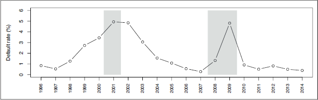
After eliminating the missing data in the covariates (which appears mainly due to different coverage of the data sources), the merged dataset contains 2528 firms and 19952 yearly observations for all firms (so-called firm-year observations), whereas the panel is highly unbalanced in the time dimension, with firms staying on average 7.89 years in the sample (see Figure A.1 in the Supplementary Material). The sample contains 375 defaults (1.88% sample default rate). Figure 1 shows the cyclical behaviour of the default rates from 1996 to 2014, with default rates increasing during and immediately after recessions.
The figure illustrates the dynamics of the default rates from 1996 to 2014. The grey shaded areas represent recession periods as indicated by the NBER based Recession Indicators for the US and correspond to the burst of the dot-com bubble and the sub-prime mortgage crisis
The figure illustrates the dynamics of the default rates from 1996 to 2014. The grey shaded areas represent recession periods as indicated by the NBER based Recession Indicators for the US and correspond to the burst of the dot-com bubble and the sub-prime mortgage crisis
There is a high rating agreement in the sample with Spearman's correlation higher than 90% for all pairs of raters. Not all ratings are observed for all firm-years, with 97.52% of the firm-years being rated by S&P, 58.67% by Moody's and 17.17% by Fitch. For all CRAs the number of ratings falling into the best and worst classes is small so for the analysis we use the following aggregated rating classes: AAA/A, BBB, BB, B, CCC/C and Aaa/A, Baa, Ba, B, Caa/Ca, respectively. The rating distribution for S&P and Moody's ratings is relatively stable over the sample period, while Fitch assigns more favourable ratings especially at the beginning of the period (Figure A.2 in the Supplementary Material shows the yearly distribution of the aggregated rating grades). Finally, the aggregated ratings change rarely: the S&P rating changes on average 0.712 times per firm, 60.4% of which are upgrades; the Moody's rating changes on average 0.747 times, 43.4% of which are upgrades; the Fitch rating changes on average 0.106 times, 62.1% of which are upgrades.
In the sample, we also observe that defaulted firms exhibit on average higher liabilities ratios (LCT/TA, F/TA, TL/MTA), higher stock price volatility, lower stock prices as well as negative income ratios and negative excess returns. The summary statistics of the covariates for both the entire and the defaulted sample are presented in Table A.1 in the Supplementary Material.
Posterior mean and posterior standard deviation of the regression coefficients β and of the coefficients γS&P, γMoody’s and γFitch of the rater bias
Posterior mean and posterior standard deviation of the regression coefficients β and of the coefficients γS&P, γMoody’s and γFitch of the rater bias
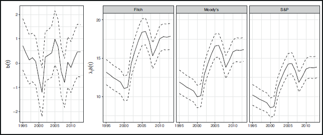
The posterior mean and the 80% symmetric credible intervals for the market factor
This figure shows the posterior mean and the 80% symmetric credible intervals for the latent systematic factor
and the scaled rater factor
at the end of each year over the period 1995 to 2013
The posterior summaries of the other parameters are presented in Table A.2 of the Supplementary Material.
For comparison purposes, we formulate several alternative model specifications which differ from the proposed modelling framework in the specification of the random effect
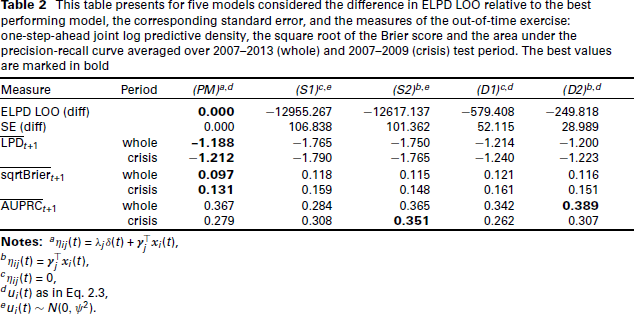
This table presents for five models considered the difference in ELPD LOO relative to the best performing model, the corresponding standard error, and the measures of the out-of-time exercise: one-step-ahead joint log predictive density, the square root of the Brier score and the area under the precision-recall curve averaged over 2007–2013 (whole) and 2007–2009 (crisis) test period. The best values are marked in bold
This table presents for five models considered the difference in ELPD LOO relative to the best performing model, the corresponding standard error, and the measures of the out-of-time exercise: one-step-ahead joint log predictive density, the square root of the Brier score and the area under the precision-recall curve averaged over 2007–2013 (whole) and 2007–2009 (crisis) test period. The best values are marked in bold
In order to compare the proposed joint model with the above models in terms of out-of-time performance, we set up a cross-validation exercise as described in Section 3.2 and start by training the model on the period 1995–2006 and then sequentially add one sample year of data to the training set. This results in seven training and test samples. Table 2 presents the one-step-ahead joint and marginal LPD averaged over all test samples (i.e., over the period 2007–2013) and over test samples covering the financial crisis 2007–2009, respectively. Similarly, we report the average one-step-ahead square root of the Brier score and area under the precision-recall curve based on the conditional probabilities of default. We observe that the proposed model (PM) performs best out-of-time in terms of the joint log predictive density scores, and more generally, the models with a dynamic specification in the PD score are better in terms of predictive performance than the static models (S1) and (S2). Model (PM) also performs best in terms of calibration, as it achieves the lowest Brier score on average over all samples and over the crisis period. In terms of discriminatory power, the static model (S2) performs best for the crisis years, while dynamic model (D2) performs best for the whole test period. This suggests that including a time-varying rater factor in the rater bias specification does not necessarily improve the ability of the model to discriminate between defaults and non-defaults.
In this article we present a joint analysis of defaults and credit ratings for a sample of US publicly traded corporates by considering a multidimensional longitudinal model of multivariate ordinal data. We integrate both default and forward-looking credit rating data in a joint statistical model and employ a dynamic specification in the latent creditworthiness equation and in the rater bias. Bayesian methods implemented in the
Future research avenues include the incorporation of a wide range of covariates in the model and tackling the issue of variable selection to allow a data-driven identification of relevant factors for both the latent PD score and the rater biases as well as the exploration of more flexible mixed-effect specifications for the latent PD score, for example, more general parameterizations for the factor loading
Footnotes
Acknowledgments
Supplementary materials for this article are available from
Declaration of conflicting interests
The authors declared no potential conflicts of interest with respect to the research, authorship and/or publication of this article.
Funding
The authors disclosed receipt of the following financial support for the research, authorship and/or publication of this article: This research was funded in part by the Austrian Science Fund (FWF) [Grant id ZK35]. For the purpose of open access, the authors have applied a CC BY public copyright licence to any Author Accepted Manuscript version arising from this submission.
Supplementary materials
Supplementary materials for this article are available from