Mixture models and networks: The stochastic blockmodel

Abstract

Mixture models are probabilistic models aimed at uncovering and representing latent subgroups within a population. In the realm of network data analysis, the latent subgroups of nodes are typically identified by their connectivity behaviour, with nodes behaving similarly belonging to the same community. In this context, mixture modelling is pursued through stochastic blockmodelling. We consider stochastic blockmodels and some of their variants and extensions from a mixture modelling perspective. We also explore some of the main classes of estimation methods available and propose an alternative approach based on the reformulation of the blockmodel as a graphon. In addition to the discussion of inferential properties and estimating procedures, we focus on the application of the models to several real-world network datasets, showcasing the advantages and pitfalls of different approaches.

1 Introduction

The underlying idea of a mixture model is rather simple. Instead of assuming that the target variable follows a plain distribution, one considers a mixture of multiple distributions. Specifically, for a random variable Y, one assumes

$$\begin{array}{cc}Y\sim \sum _{k=1}^K{\pi }_k{f}_k(y),\hfill & \hfill \end{array}$$

(1.1)

where ${\pi }_k$ is a weighting coefficient, with ${\sum }_{k=1}^K{\pi }_k=1$ , and $f_k(·)$ is the $k$ th mixture distribution. Commonly, the mixture components come from the same distributional family but differ in their parameters, that is, $f_k(·)=f(·|{\mathbf{\theta }}_k)$ , where ${\mathbf{\theta }}_k$ parametrizes the $k$ th mixture component. An early (maybe the first) reference in this direction dates back to Pearson (1894) and focuses on the estimation of a mixture of two normal distributions. An early mathematical treatment of the topic, more in the style of convolution, is provided in Robbins (1948). In a series of papers, Teicher (1960) discusses identifiability issues, where the cited work puts the focus on finite mixtures in the style of (1.1). A first survey on mixture models is provided by Gupta and Huang (1981), presenting the different estimation routines that had been developed and used by that time. A central algorithm in this respect, which is not included in the above survey article (certainly because of simultaneous time of publication), is the work of (Aitkin and Wilson (1980); see also Aitkin (1980)) who propose the use of the at the time recently developed Expectation–Maximization (EM) algorithm (see Dempster et al.(1977)Dempster, Laird, and Rubin) to estimate the finite mixture distribution. Though the focus of their paper lies in the modelling of outliers, the authors make use of the idea that a finite mixture model can be comprehended as a missing data problem. Under this modelling framework, one assumes that the discrete valued random variable $Z$ takes values $\{1,...,K\}$ with

$$\begin{array}{cc}P(Z=k)={\pi }_k,\hfill & \hfill \end{array}$$

(1.2)

where again ${\sum }_{k=1}^K{\pi }_k=1$ . Conditional on $Z=k$ , one then observes $Y$ from the $k$ th mixture component, that is,

$$\begin{array}{cc}Y|(Z=k)\sim f_k(y)\mathit{for}k=1,...,K.\hfill & \hfill \end{array}$$

Treating Z as unobserved (or unobservable) enables the framing of estimation in a missing data situation, where the considered likelihood (1.1) can be maximized with the EM algorithm. The results are generalized and extended towards hypothesis tests in Aitkin and Rubin (1985). A comprehensive overview on finite mixture models is given in the early book of Everitt and Hand (1980), followed by the monographs of Titterington et al.(1985)Titterington, Smith, and Makov, Lindsay (1995), Böhning (1999), McLachlan and Peel (2000) and Frühwirth-Schnatter (2006). We also refer to the recent Handbook of Mixture Analysis (Frühwirth-Schnatter et al.(2019)Frühwirth-Schnatter, Celeux, and Robert). For software implementations of mixture models, Leisch (2004) is a central reference (see also Benaglia et al.(2009)Benaglia, Chauveau, Hunter, and Young). Allowing the mixture components and/or the mixing proportions ${\pi }_k$ to depend on additional covariates extends mixture models towards regression models. The resulting model class is also known as mixture of experts, tracing back to Jacobs et al.(1991)Jacobs, Jordan, Nowlan, and Hinton. A survey from the perspective of machine learning can be found in Masoudnia and Ebrahimpour (2014, see also Gormley and Frühwirth-Schnatter (2019)).

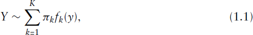
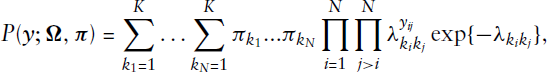
While most of the literature cited above deals with a univariate response variable Y, in this article we aim to look at multivariate data with $\mathbf{Y}$ expressing a network. Network data have a simple binary structure resulting from a network as follows. Assume a set of N actors, where we define with $V=\{v_1,...,v_N\}$ the set of nodes in a network. We call $E\subset V\times V$ the edge set, and the resulting network can be represented with an adjacency matrix $\mathbf{Y}$ such that $\mathbf{Y}\in \{0,1{\}}^{N\times N}$ and

$$Y_{\mathit{ij}}=\left\{\begin{array}{cc}1,\mathit{if}(v_i,v_j)\in E\hfill & \hfill \\ 0,\mathit{otherwise}.\hfill & \hfill \end{array}\right.$$

If the network is undirected, $Y_{\mathit{ij}}=Y_{\mathit{ji}}$ holds. Furthermore, the diagonal of $\mathbf{Y}$ often remains undefined, meaning that self-loops are not contemplated. The statistical analysis of network data has achieved increasing interest in the last two decades: We refer to Kolaczyk (2009) and Kolaczyk and Csárdi (2014) for a general introduction to the topic (see also Goldenberg et al.(2009); Hunter et al.(2008); Fienberg (2012); Lusher et al.(2013); Salter-Townshend et al.(2012); Biagini et al.(2019)).

If we consider $\mathbf{Y}$ as set of random variables $\{Y_{\mathit{ij}};1\le i,j\le N,i\ne j\}$ , we can transfer the mixture model setting (1.1) towards network data. This leads to what is commonly referred to as (a posteriori) stochastic blockmodelling. A survey on the latest theoretical developments in this field has recently been published by (Abbe (2018); see also Lee and Wilkinson (2019) for a comprehensive review). Stochastic blockmodels can be seen as a tool for performing community detection (see, e.g., Clauset et al.(2004); Fortunato (2010); Fortunato and Hric (2016)). While community detection and stochastic blockmodels have a lot in common, the latter specifically focuses on the modelling aspect and will therefore be considered here. A stochastic blockmodel (SBM) is in fact a mixture model where each mixture component is specified by the group or community membership. The latent subgroups of nodes are typically identified by their connectivity behaviour, with nodes behaving similarly belonging to the same community. The class of stochastic blockmodels evolved from its deterministic counterpart, which dates back to White et al.(1976). The stochastic version of the blockmodel was introduced by Holland et al.(1983) in the statistical literature. Similar modelling proposals, developed independently, trace back to the computer science literature (see, for example, Bui et al., 1987). Wang and Wong (1987) were the first to apply the stochastic blockmodel to directed graphs, even though they still assumed the block structure to be known. The first steps towards a posteriori blockmodelling, that is modelling with initially unknown group structure, were taken by Snijders and Nowicki (1997) and Nowicki and Snijders (2001), who proposed estimation routines for, respectively, two groups and any known number of groups. From there, the model class gained traction. Recent literature on the classical version of stochastic blockmodels includes Daudin et al.(2008), Gormley and Murphy (2010) and Aitkin et al.(2014), using Bayesian approaches (see also Vu and Aitkin (2015)). Following their initial formulation, stochastic blockmodels have been extended in various ways. Some of such variants and extensions will be reviewed and treated in Section 3, and some of those will be put to practice later on. The aim of this article is to illuminate on the connection between mixture models and stochastic blockmodels, exploring some of the different approaches within the model class and demonstrating their applicability by making use of real data. The article also introduces a different formulation of the stochastic blockmodel through the graphon framework, using this reformulation to propose an alternative estimation routine.

The rest of the article is organized as follows: Section 2 presents some real-world network datasets together with the potential questions that we face in analysing them. Those datasets will be later used to demonstrate the capabilities of stochastic blockmodels. Section 3 describes the blockmodelling framework in more detail, and introduces some of its most prominent variants and extensions. Section 4 compares the different estimation routines that are available, and introduces a Monte Carlo-based EM estimation routine under graphon representation. The empirical analysis of the previously introduced datasets is then carried out in Section 5, making use of the previously described models to tackle the questions posed in Section 2. Finally, Section 6 ends the article with some comments and conclusive remarks.

2 Data description

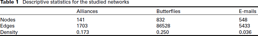
In order to demonstrate the capabilities of stochastic blockmodels, we have chosen network datasets pertaining to three different domains, namely political science, biology and sociology. Despite the different domains, the networks share the presence of some form of underlying community structure, or at least the appearance thereof. They all therefore lend themselves to be modelled through the use of mixture components. General descriptive measures of the data examples, which consist of undirected graphs, are given in Table 1, which shows that all three networks are of medium size and range from very dense to relatively sparse.

Table 1:

Descriptive statistics for the studied networks

Nodes	141	832	548
Edges	1703	86528	5433
Density	0.173	0.250	0.036

2.1 International alliances network

The first network that we introduce is constructed using data from the Alliance Treaty Obligations and Provisions project (Leeds et al.(2002)). The dataset provides information on military alliance agreements pertaining to all countries of the world. For the analysis we consider alliances that were in force in the year 2016. The countries are taken as nodes, and an edge between two countries is present if the two countries take part in a ‘strong’ military alliance treaty. More specifically, the alliances that we consider strong are defensive and offensive ones. This means, respectively, ‘\textsl alliances in which the members promise to provide active military support in the event of attack on the sovereignty or territorial integrity of one or more alliance partners’ and ‘\textsl alliances in which the members promise to provide active military support under any conditions not precipitated by attack on the sovereignty or territorial integrity of an alliance partner, regardless of whether the goals of the action are to maintain the status quo’ (see Leeds et al.(2002)). Note that, in general, an alliance can involve more than two nodes: Representing the network using dyadic edges only thus leads to the loss of some information. For example, pairwise edges between countries $i$ , $j$ and $k$ could mean three pairwise treaties, or a treaty that involves all three of them. While using pairwise edges as we do here is standard in network modelling, hypergraph representations (Berge (1984)) offer a viable alternative, and models representing this kind of data in a more natural way have been explored (see, e.g., Chodrow (2020)). Looking at the network from a blockmodelling perspective, there are several questions that we can pose. First of all, do alliances between countries induce a partition of the network that is meaningful from a geopolitical perspective? Moreover, will the blocks found be in line with geographic proximity and political affinity, or will there be some other characteristics driving the grouping? And finally, what can the resulting block structure tell us about the global system of alliances?

2.2 Butterfly similarity network

The second real-world instance is a butterfly similarity weighted network, constructed using the data presented by Wang et al.(2009) and available from Zitnik et al.(2018). Each node represents a butterfly, and valued edges depict visual similarities between them. More specifically, pairs of butterflies with some positive degree of similarity between them are connected by a weighted edge, while no edge is present if the similarity score between the two is zero. The absence of an edge is thus equivalent to the presence of an edge with weight zero. The similarity scores lie in the interval $[0,1.55]$ , with a higher value implying a higher degree of similarity. Scores are computed using butterfly images, as described in Wang et al.(2009). Information on the species to which each butterfly belongs is also available, with each unit belonging to a single species. A total of ten species are present, implying a ‘natural’ partition of the network in ten blocks. In this case, there is one clear question that emerges: Are the communities found using visual similarity scores in agreement with how biologists categorized butterfly species? In other words, are we able to recover the ‘ground truth’ communities of the network via stochastic blockmodelling?

2.3 Email exchange network

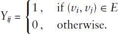
The last network considered consists of anonymized email data from a large European research institution, collected between October 2003 and May 2005 (Leskovec and Krevl (2014)). Each node in the network represents a person, and an edge between nodes $i$ and $j$ is present if person $i$ sent person $j$ at least one email in the examined period. The nodes featured in this network are all members of the institution, meaning that only emails within the institution itself are considered. Moreover, only nodes belonging to the largest ten departments are included. Note that, similarly as for the previously described alliances data, this binary representation disregards the multi-dimensional nature of the edges (as an email can have multiple recipients). Since department memberships are known and individuals from the same department are expected to behave similarly, we can consider the departments as ‘ground truth’ communities for the network. Given that, the questions that we pose are straightforward: Are we able to find some form of meaningful community structure in the network considering emails alone? And if so, will the structure recovered be similar to the partition induced by department memberships? And finally, what can email exchanges tell us about the structure of the institution and the relationships between departments? To analyse this and the other previously introduced networks and to investigate the correspondingly raised questions, we will introduce the appropriate model variants and related estimation procedures in the following sections.

3 Stochastic blockmodels: formulations and variants

3.1 The standard stochastic blockmodel

As anticipated in the introduction, if we consider the network $\mathbf{Y}$ as set of random variables $\{Y_{\mathit{ij}};1\le i,j\le N,i\ne j\}$ , we can transfer the mixture model setting (1.1) towards network data. This leads to the stochastic blockmodel, that is a mixture model for which each mixture component is specified by the group or community membership. More specifically, we assume the independent discrete group indicator coefficients $Z_i\in \{1,...,K\}$ for $i=1,...,N$ with

$$\mathbb{\mathbb{P}}(Z_i=k)={\pi }_k\mathit{for}k=1,...,K$$

and, as above, ${\sum }_{k=1}^K{\pi }_k=1$ . An edge between node $i$ and $j$ then exists with probability

$$\begin{array}{cc}{Y}_{\mathit{ij}}|(\mathbf{Z}=\mathbf{z})\sim \mathit{Bernoulli}(p_{z_i{z}_j}),\hfill & \hfill \end{array}$$

(3.1)

where $\mathbf{P}=[p_{\mathit{kl}}{]}_{k,l=1,\dots ,K}$ is the $K\times K$ dimensional block-probability matrix. For community detection one typically assumes that $p_{\mathit{kk}}>p_{\mathit{kl}}$ for all $l\ne k$ , but this is not a requirement for stochastic blockmodels in general. In fact, the block structure may describe clusters of nodes that behave similarly from a connectivity standpoint without necessarily being more densely connected, thus allowing for other types of structures, such as disassortative communities and core-periphery.

For estimation, a numerically simpler setting can result by approximating the binomial distribution through a Poisson distribution. This approximation is justified since the network density is usually low, implying that $p_{\mathit{kl}}$ is typically small. In this case, (3.1) is replaced by

$$\begin{array}{cc}{Y}_{\mathit{ij}}|(\mathbf{Z}=\mathbf{z})\sim \mathit{Poisson}({\lambda }_{\mathit{ij}}),\hfill & \hfill \end{array}$$

(3.2)

where ${\lambda }_{\mathit{ij}}=\text{exp}\left\{{\omega }_{z_i{z}_j}\right\}$ , with $\mathbf{\Omega }=[{\omega }_{\mathit{kl}}{]}_{k,l=1,\dots ,K}$ as block-connectivity para\-meter matrix. One of the main allures of the Poisson model variant lies in the fact that there is a closed form for integrating out parameters, as seen in, for example, (McDaid et al.(2013); see also Lee and Wilkinson (2019) for an illustration of this).

3.2 Degree correction

A well-known extension of the classical SBM is the degree-corrected stochastic blockmodel, introduced by Karrer and Newman (2011). In their work, the authors show how the standard stochastic blockmodel implicitly assumes the degree structure within communities to be relatively homogeneous. This, combined with the fact that many real-world networks exhibit extremely skewed degree distributions (Simon (1955); Barabási and Albert (1999)), leads the model to often only be able to find core-periphery type block structures, where node grouping is predominantly driven by degree similarity. To bypass this issue, Karrer and Newman (2011) introduced the idea of degree correction, making the probability of an edge depend not only on group membership, but also on node-specific heterogeneity parameters. More precisely, the original version of the degree-corrected SBM can be written in the same way as (3.2), but in this case

$$\begin{array}{cc}{\lambda }_{\mathit{ij}}=\text{exp}\left\{{\gamma }_i+{\gamma }_j+{\omega }_{z_i{z}_j}\right\}.\hfill & \hfill \end{array}$$

(3.3)

In this notation $\text{exp}\left\{{\gamma }_i\right\}$ quantifies the heterogeneity specific of node $i$ , and $\text{exp}\left\{{\omega }_{z_i{z}_j}\right\}$ can be viewed as a measure of the propensity to form ties between the groups to which nodes $i$ and $j$ belong. Note that the degree-corrected SBM is not, in general, strictly better than the standard one, as the two models imply different underlying structures of the network (see, e.g., Yan et al.(2014); Yan (2016); Wang and Bickel (2017)). The choice of one over the other simply depends on what is the kind of structure one wishes to find. It is also possible to combine the two approaches, as done in Aicher et al.(2015) and Lu and Szymanski (2019). All three versions of the model, namely (3.1), (3.2) and (3.3), will be applied to the previously introduced data examples.

3.3 Graphon representation

The stochastic blockmodel can also be formulated through the graphon model class, which recently received a lot of attention concerning the modelling of complex networks. Although the scope of the structures representable as a graphon is quite large, its formulation is rather simple. Let us therefore introduce $U_i$ , for $i=1,\dots ,N$ , as node-specific continuous random variables which can be described as

$$U_i\stackrel{\text{ i}\text{.i}\text{.d}\text{. }}{\sim }\text{ Uniform }[0,1]$$

(3.4)

The network entries are then assumed, conditionally and independently from one another, to follow

$$\begin{array}{c}\hfill Y_{\mathit{ij}}|(\mathbf{U}=\mathbf{u})\sim \mathit{Bernoulli}(p(u_i,u_j)),\hfill \end{array}$$

where $p:[0,1]\times [0,1]\to [0,1]$ is a function (sometimes called graphon). This function $p(·,·)$ is commonly assumed to be at least piecewise continuous, meaning to fulfill some Lipschitz or Hölder condition in segments. A representation of the SBM can then be generated by restricting the graphon function to be locally constant in a rectangular pattern. More precisely we define, for a SBM with K groups,

$$\begin{array}{cc}p(u_i,u_j)=\sum _{k=1}^K\sum _{l=1}^K{1}_{\{{\tau }_{k-1}\le u_i<{\tau }_k\}}{1}_{\{{\tau }_{l-1}\le u_j<{\tau }_l\}}{p}_{\mathit{kl}}\hfill & \hfill \end{array}$$

(3.5)

with $1_{\{·\}}$ as indicator function, $0={\tau }_0<{\tau }_1<\dots <{\tau }_K=1$ as boundaries, and $p_{\mathit{kl}}$ representing the edge probability between and within groups, as defined above. The group memberships $Z_i$ are here substituted by the node-specific quantities $U_i$ , which are also latent. This additionally implies that the community proportions are now represented by the boundaries ${\tau }_k$ , $k=1,\dots ,K-1$ . Note that from the uniform distribution of $U_i$ specified in (3.4) follows that ${\tau }_k={\sum }_{l=1}^k{\pi }_l$ . An instance of such relationship can be given through the following illustration:

Figure 1.

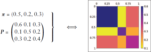
It is thus not difficult to see how this formulation of graphon models is equivalent to SBMs.

In this context, it should be noted that the graphon model suffers from major identifiability issues, which, with regard to the SBM representation, also include the label switching problem (we refer to the Appendix for more details and illustrations). This non-identifiability arises from the fact that any permutation of $p(·,·)$ represents the same network-generating model as $p(·,·)$ itself. Even more generally, two graphon functions $p(·,·)$ and $\tilde{p}(·,·)$ represent the same network-generating model if and only if there exist two measure preserving functions $\varphi ,\tilde{\varphi }:[0,1]\to [0,1]$ such that $p(\varphi (u),\varphi (v))=\tilde{p}(\tilde{\varphi }(u),\tilde{\varphi }(v))$ for almost every $(u,v)\in [0,1{]}^2$ (Diaconis and Janson (2008)). A common approach to resolve this issue is the postulation of a monotonically non-decreasing marginal function $g(u)={\int }_0^{1}p(u,v)dv$ (see, e.g., Bickel and Chen (2009) or Chan and Airoldi (2014)). With regard to SBMs, that means ordering the communities, $k=1,\dots ,K$ , by ${\sum }_{l=1}^K{p}_{\mathit{kl}}\Delta {\tau }_l$ with $\Delta {\tau }_l={\tau }_l-{\tau }_{l-1}$ , inducing the additional constraint of ${\sum }_{l=1}^K{p}_{\mathit{kl}}\Delta {\tau }_l\ne {\sum }_{l=1}^K{p}_{\mathit{jl}}\Delta {\tau }_l$ for all $k\ne j$ . This assumption, however, might yield only an imperfect identification, especially when the marginal functions ${\sum }_{l=1}^K{p}_{\mathit{kl}}\Delta {\tau }_l$ are similar (see Nowicki and Snijders (2001)). Moreover, this is a strong restriction to the generality of graphon models. We therefore aim to circumvent this issue by formulating an adequate estimation procedure (see Section 4.3).

3.4 Further variants and extensions

Many other variants and extensions of SBMs exist. These include the mixed membership model (Airoldi et al.(2008)), in which nodes can belong to multiple communities simultaneously, and the hierarchical stochastic blockmodel (Peixoto (2017)), in which communities are comprised of meta-communities, leading to a hierarchical block structure. A matter of simplifying the model representation is what motivates the microcanonical variant of the SBM (see, e.g., Peixoto (2012)), where the structural pattern is strictly fixed in absolute values. This, in turn, allows for fitting more elaborate generative models, which usually require Markov Chain Monte Carlo (MCMC) techniques for evaluation, to larger networks and to an increased number of groups, as demonstrated by Peixoto (2017). The same author also proposed a nested hierarchical variant of the SBM (Peixoto(2014a)) in which the generative model inferred at an upper level serves as prior information to the one at a lower level, thus also providing an increased resolution when performing model selection. Despite its more elaborate formulation, this hierarchical model remains tractable, and it is feasible to apply it to very large networks. It is also possible to add covariates to the analysis, as initially proposed by Tallberg (2005) and further elaborated by Choi et al.(2012), Sweet (2015) and Huang and Feng (2018). A further extension is the mixture of experts SBM (see Gormley and Murphy (2010); White and Murphy (2016)), which allows covariates to enter the latent position cluster model in a number of ways, yielding different model interpretations. Extensions for more specific purposes have also been developed: Bouveyron et al.(2018) introduced the stochastic topic blockmodel, a probabilistic model for networks with textual edges. Their model addresses the problem of discovering meaningful clusters of vertices that are coherent with regards to both the network interactions and the text contents. Finally, another relevant approach that can be seen as a generalization of the SBM is the latent position cluster model proposed by Handcock et al.(2007) (originating from Hoff et al.(2002), see also Krivitsky et al.(2009)). It is worth noting that most of the mentioned specifications can be applied to binary data as well as to valued and count data (see, e.g., Nowicki and Snijders (2001)). In this article, we do not concentrate on these extensions, but focus on the more ‘classical’ SBMs.

4 Estimation techniques

4.1 Variational methods

The EM algorithm proved to be a powerful and numerically efficient way for estimating parameters in mixture models (see Aitkin (1980) or Friedl and Kauermann (2000)). Unfortunately, this does not extend to the estimation of stochastic blockmodels. The complete data log-likelihood resulting from (3.2) in the case of an undirected network equals

$$\begin{array}{cc}{l}_C(\mathbf{\Omega },\mathbf{\pi })=\sum _{i=1}^N\sum _{j=i}^N\sum _{k,l=1}^K{1}_{\{z_i=k\}}{1}_{\{z_j=l\}}(y_{\mathit{ij}}{\omega }_{\mathit{kl}}-\text{exp}\{{\omega }_{\mathit{kl}}\})+\sum _{i=1}^N\sum _{k=1}^K{1}_{\{z_i=k\}}\text{log}({\pi }_k)\hfill & \hfill \end{array}$$

(4.1)

with the side constraint ${\sum }_{k=1}^K{\pi }_k=1$ . Applying the EM algorithm would in this case mean calculating the posterior distribution

$$P(Z_i=k,Z_j=l|\mathbf{Y}=\mathbf{y})$$

with $\mathbf{y}$ being the observed adjacency matrix. This posterior, due to the resulting dependence structure of $Z_i$ and $Z_j$ , is numerically intractable (Mariadassou et al.(2010)Mariadassou, Robin, and Vacher). To circumvent such numerical hurdles, Jordan et al.(1999) proposed variational methods, which are based on an approximation of the likelihood. Let $P(\mathbf{y};\mathbf{\Omega },\mathbf{\pi })$ be the probability of the data, resulting through

$$P(\mathbf{y};\mathbf{\Omega },\mathbf{\pi })=\sum _{k_1=1}^K\dots \sum _{k_N=1}^K{\pi }_{k_1}...{\pi }_{k_N}\prod _{i=1}^N\prod _{j>i}^N{\lambda }_{k_i{k}_j}^{y_{\mathit{ij}}}\text{exp}\left\{-{\lambda }_{k_i{k}_j}\right\},$$

which is apparently too complex from a numerical perspective. We define the lower bound function

$$J(\tilde{P}(\mathbf{z};\mathbf{\xi });\mathbf{\Omega },\mathbf{\pi })=\text{log}P(\mathbf{y};\mathbf{\Omega },\mathbf{\pi })-\mathit{KL}(\tilde{P}(\mathbf{z};\mathbf{\xi }),P(\mathbf{z}|\mathbf{y};\mathbf{\Omega },\mathbf{\pi })),$$

where $\mathit{KL}(·,·)$ defines the Kullback–Leibler divergence. If we choose $\tilde{P}(\mathbf{z};\mathbf{\xi })$ to be the posterior distribution of $\mathbf{Z}$ given $\mathbf{\xi }$ , we obtain $J(;)$ to be equal to the log-likelihood of the observed data. Since this is numerically problematic, we compute the posterior distribution of $\mathbf{Z}$ given $\mathbf{\xi }$ through independence:

$$\tilde{P}(\mathbf{z};\mathbf{\xi })=\prod _{i=1}^N\prod _{k=1}^K{{\mathbf{\xi }}_k}^{1_{\{z_i=k\}}},$$

where ${\mathbf{\xi }}_k=({\xi }_{k1},...,{\xi }_{\mathit{kN}})$ is a vector containing the probabilities for each of the N nodes to be in group $k$ , with ${\sum }_{k=1}^K{\xi }_{\mathit{ki}}=1$ needing to hold for every $i\in 1,...,N$ . $\mathbf{\xi }=({\mathbf{\xi }}_1,\dots ,{\mathbf{\xi }}_K)$ is known as variational parameter, and needs to be chosen such that $J(\tilde{P}(\mathbf{z};\mathbf{\xi });\mathbf{\Omega },\mathbf{\pi })$ is maximized with respect to all parameters. It can be shown that $J(;)$ can, up to an intractable constant, be written in a simple numerical form which allows for fast and numerically feasible estimation. The remaining unknown component expresses the approximation error which is typically difficult to quantify (see Lee et al.(2020)).

4.2 Vertex switching algorithms

Another possibility for the estimation of stochastic blockmodels is to maximize the likelihood through vertex switching routines. The basic idea of this type of algorithms is the following: starting from an initial, possibly random group assignment, a starting value of the likelihood is computed. From there, one or more vertices are moved from one group into another, and the likelihood is computed again. The new allocation is then accepted or rejected based on a function of the previous and the subsequent likelihood, and such procedure runs iteratively until convergence is reached, that is until a maximum is found. Algorithms of this type include single-vertex Monte Carlo (see, e.g., Peixoto (2013), 2014b) and a local heuristic routine inspired by the Kernighan–Lin algorithm used in minimum-cut graph partitioning (Kernighan and Lin (1970); Karrer and Newman (2011)). In principle, computing the likelihood that many times may seem quite expensive. On the other hand, it is not always necessary to calculate the complete likelihood at each step. Depending on the model specification, it is often possible to write the change in the likelihood in a computationally efficient way, so that the algorithm becomes quite competitive in terms of speed. The chief issue with this type of algorithm is that, given the heuristic maximization routine, it is not possible to obtain a measure of uncertainty for group assignments. The procedure will only produce the graph partitioning that (locally) maximizes the likelihood, without any additional information. This is fine if the problem at hand is one of pure community detection, but can become problematic if the goal is proper mixture modelling, as the stochastic component of the mixture is lost. Another potential issue is the possibility to get stuck at local maxima, which usually is tackled by running the procedure several times with different (random) starting points.

4.3 Monte–Carlo-based EM estimation under graphon representation

A third and to some extent novel estimation routine is to estimate the block structure using its graphon representation. Although it is not quite clear how this approach competes with already existing methods, our ambition here is to demonstrate a further possible form of representing and estimating mixture models in networks. Such a model can be fitted appropriately by applying an EM-type algorithm including Gibbs sampling in the E-step. As mentioned above, EM-based algorithms are a common approach to estimate mixture models as well as other models involving latent variables, although in the case of networks the task becomes analytically intractable and numerically demanding. We therefore make use of MCMC techniques to approximate the complex posterior distribution of the latent quantities, which here reflect the group assignments. In this approach, we thus slightly reformulate the stochastic blockmodelling procedure, relating it to graphon estimation (see, e.g., Latouche and Robin (2016) or, for the reverse link, Olhede and Wolfe (2014) and Airoldi et al.(2013)). We here want to follow the estimation approach of Sischka and Kauermann (2019), applying it to SBMs. The idea is to make use of model (3.4) and estimate, in the M-step, the parameters of 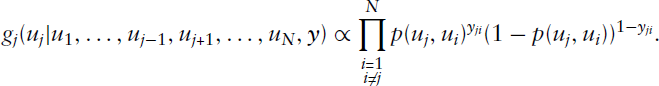$p(·,·)$ , namely the interval boundaries ${\tau }_k$ and the blockwise heights $p_{\mathit{kl}}$ , $k,l=1,\dots ,K$ , directly yielding estimates for the SBM quantities $\mathbf{\pi }$ and $\mathbf{P}$ . The group assignments $Z_1,\dots ,Z_N$ can be determined by considering the positions $U_1,\dots ,U_N$ in relation to $\mathbf{\tau }=({\tau }_0,\dots ,{\tau }_K)$ . To carry out the E-step, we assume the function $p(·,·)$ to be given (or to be set to the current estimate). In this regard, as follows from (3.4), the full conditional posterior can be formulated as

$$g_j\left(u_j|u_1,\dots ,u_{j-1},u_{j+1},\dots ,u_N,y\right)\propto {\displaystyle \prod _{\begin{array}{l}i=1\\ i\ne j\end{array}}^{N}p{\left(u_j,u_i\right)}^{y_{ii}}}{\left(1-p\left(u_j,u_i\right)\right)}^{1-y_{ji}}.$$

This allows for applying Gibbs sampling in a straightforward manner. Details on this sampling scheme, as well as remarks on the associated potential issues of label switching and non-identifiability, are given in the Appendix. In this context, we underline how the issue of label switching is prevented through the EM algorithm on the primary level of the estimation procedure (apart from the exceptional case of complete symmetry, as described in the Appendix). In comparison, label switching is a common problem when making use of an overall Bayesian estimation procedure (if the MCMC scheme is run for sufficiently long, see Stephens (2000)), where one randomly draws quantities from the corresponding posterior distributions in alternating fashion. This, in contrast, is circumvented in the EM framework, since in the E- and M-steps the results of the respective other step are kept fixed and, based on that, the ‘optimal’ solution is carried out to be used for the next iteration. Parameter estimates are thus not achieved by averaging over several iterations but are given for each iteration separately. Therefore, with regard to our estimation routine, no post-hoc relabelling is required, and assignments can be adopted as deduced from the subordinate Gibbs sampling scheme. Making use of the sampling sequence, we specify the posterior mode in the mth iteration using 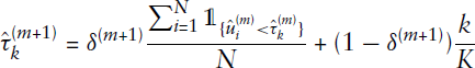${\widehat{u}}_j^{(m)}=({\tau }_{k^{\prime }-1}+{\tau }_{k^{\prime }})/2$ for $j=1,\dots ,N$ , where the index $k^{\prime }$ is defined as ${\mathit{arg}\mathit{max}}_k{\sum }_{t=1}^n{1}_{\{{\tau }_{k-1}\le u_j^{<t·r>}<{\tau }_k\}}$ . In that regard, $u_j^{<t>}$ is the value of the $j$ th element in the Markov chain at time $t$ , and $n\in \mathbb{}$ is the number of considered states of the MCMC sequence extracted by thinning factor $r\in \mathbb{}$ . To take into account that the $U_i$ are uniformly distributed and therefore expected to spread proportionally to interval size, we additionally apply a subsequent adjustment. This concerns both the latent quantities $U_i$ and the interval boundaries ${\tau }_1,\dots ,{\tau }_{K-1}$ . Assuming that ${\widehat{\tau }}_k^{(m)}$ represents the current estimate of ${\tau }_k$ , we then set

$$\begin{array}{c}\hfill {\widehat{\tau }}_k^{(m+1)}={\delta }^{(m+1)}\frac{{\sum }_{i=1}^N{1}_{\{{\widehat{u}}_i^{(m)}<{\widehat{\tau }}_k^{(m)}\}}}{N}+(1-{\delta }^{(m+1)})\frac{k}{K}\hfill \end{array}$$

and accordingly adjust the estimates of $U_j$ in the form of ${\tilde{\widehat{u}}}_j^{(m)}=({\widehat{\tau }}_{k^{\prime }-1}^{(m+1)}+{\widehat{\tau }}_{k^{\prime }}^{(m+1)})/2$ , with index $k^{\prime }$ defined through the previous assignment in the form of ${\widehat{u}}_j^{(m)}\in [{\widehat{\tau }}_{k^{\prime }-1}^{(m)}+{\widehat{\tau }}_{k^{\prime }}^{(m)})$ . Regarding the specification of ${\widehat{\tau }}_k^{(m+1)}$ , the weighting ${\delta }^{(m+1)}\in [0,1]$ with ${\delta }^{(m+1)}\ge {\delta }^{(m)}$ induces a step-size adaptation from a priori equidistant boundaries to observed boundaries implied by frequencies. Such step-size adaptation is recommendable to prevent the community size to shrink too substantially before the structure of the community has been evolved properly. In general, ${\delta }^{(m)}$ is chosen to be one in the last iteration.

The M-step is then carried out by maximizing the likelihood conditionally on 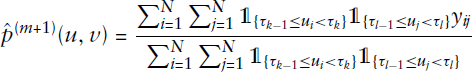$\mathbf{U}={\widetilde{\widehat{\mathbf{u}}}}^{(m)}$ and for ${\tau }_1,\dots ,{\tau }_{K-1}$ , taking the estimates adjusted as above. This is easily done by setting

$$\begin{array}{cc}{\widehat{p}}^{(m+1)}(u,v)=\frac{{\sum }_{i=1}^N{\sum }_{j=1}^N{1}_{\{{\tau }_{k-1}\le u_i<{\tau }_k\}}{1}_{\{{\tau }_{l-1}\le u_j<{\tau }_l\}}{y}_{\mathit{ij}}}{{\sum }_{i=1}^N{\sum }_{j=1}^N{1}_{\{{\tau }_{k-1}\le u_i<{\tau }_k\}}{1}_{\{{\tau }_{l-1}\le u_j<{\tau }_l\}}}\hfill & \hfill \end{array}$$

for all $u\in [{\tau }_{k-1},{\tau }_k)$ and $v\in [{\tau }_{l-1},{\tau }_l)$ . As it is done for the previously mentioned vertex switching algorithms, we run this MCEM algorithm several times with varying initialization of $\mathbf{U}$ , and then choose the outcome with the highest likelihood, which should here also prevent us from getting stuck at a local maximum. To determine the optimal number of blocks, typical model selection criteria can be applied. We here make use of the AIC, for which both quantities required for the computation, namely the likelihood and the number of parameters, can easily be determined. The major advantage of the reformulation of model (3.1) to model (3.4) is that the graphon function $p(·,·)$ could be also formulated in more complex fashion, that is, instead of just being local constant one could allow for more complex structures within each segment. This is not pursued in this article, but we refer to this new research strand discussed, among others, in Vu et al.(2013).

In contrast to non-stochastic estimation routines, such as the vertex switching algorithm discussed in Section 4.2, this modelling approach naturally yields information about the inherent uncertainty of the proposed group allocation. In order to achieve this, we run the E-step one more time after the algorithm has converged. The resulting Gibbs sampling sequence of this last iteration then reveals the distribution of the node allocation with respect to the model estimate $(\widehat{p}(·,·),\widehat{\mathbf{\tau }}=(0,{\widehat{\tau }}_1,\dots ,{\widehat{\tau }}_{K-1},1))$ . A normalized Gini coefficient calculated over the assignment frequencies of a single vertex can then be used as a measure of uncertainty, where a value near one (zero) implies a low (high) level of uncertainty.

4.4 Choosing the number of blocks

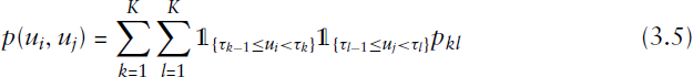
A general big challenge in mixture models (and hence also in stochastic blockmodels) lies in the choice of the number of mixture components (blocks). In fact, most of the variants presented so far require that number to be known a priori. This is typically not true in real-world applications. In mixture models the question of choosing the number of mixture components is tackled, for instance, in Aitkin (2011). In the field of stochastic blockmodels, a comprehensive list of different approaches is provided by Lee and Wilkinson (2019). Approaches based on penalized likelihood criteria have emerged. In particular, Wang and Bickel (2017) consider an approach based on the log-likelihood ratio statistic, enabling the use of a likelihood-based model selection criterion that is asymptotically consistent. Other techniques are also available: Chen and Lei (2018) develop a network cross-validation approach which is based on a block-wise node-pair splitting technique, combined with an integrated step of community recovery using sub-blocks of the adjacency matrix. Mariadassou et al.(2010) base the choice on an Integrated Classification Likelihood criterion. The number of blocks can also be estimated using ‘collapsed’ approaches, where the model parameters are integrated out in a Bayesian formulation of the model. The model space and cluster allocations can then be estimated using a greedy search routine (Côme and Latouche (2015)) or using MCMC (McDaid et al.(2013)). Another possible approach is that of Peixoto (2013), who uses the Minimum Description Length principle, which seeks to minimize the total amount of information required to describe the network and avoid overfitting. This also allows to deduce general bounds on the detectability of any prescribed block structure, given the number of nodes and edges in the sampled network. Finally, Riolo et al.(2017) (see also Newman and Reinert (2016)) present a method for estimating the number of communities in a network using a combination of Bayesian inference and an efficient Monte Carlo sampling scheme. While other approaches have been proposed, we will not go into further detail here. For modelling the previously described networks, when possible we select K such that the resulting number of blocks coincides with the ground truth. If such ground truth is not available, we make use of the Akaike Information Criterion (AIC), which can be easily calculated when using the graphon representation-driven algorithm.

5 Application to real world networks

5.1 International alliances network

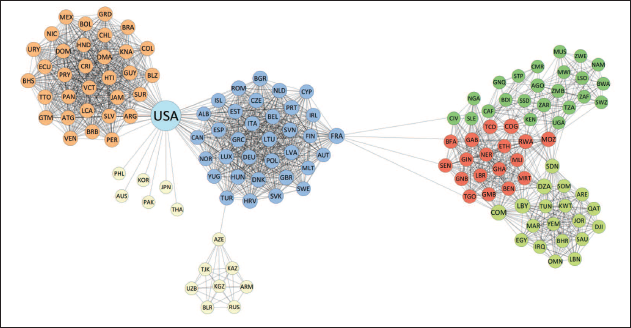
To model the network we use the standard version of the stochastic blockmodel, as in (3.1). Estimation was performed using the Monte Carlo-based EM routine under graphon representation. Applying the AIC yields seven communities as the optimal dimensionality of the blockmodel. The resulting fitted block decomposition is given in Figure 1. Network visualization, as for the rest of the examples in this section, is carried out through use of the open-source tool Gephi (Bastian et al.(2009)). The associated world map is shown in Figure 2, where countries are coloured by block. States coloured in grey on the map are isolates in the network, meaning that they were not involved in any strong military alliance in 2016. Moreover, China, Cuba and North Korea are only connected to each other, and are thus isolated from the rest of the network. Those countries have therefore been excluded from the model fitting.

Figure 1:

Global network of political alliances in 2016. Two countries are connected if they have taken part in a strong alliance treaty. Labels indicate country codes, while nodes are coloured by block memberships found through the standard stochastic blockmodel

The plots show how the blocks recovered by the stochastic blockmodel are very much related and in accordance with the geopolitical structure of the modern world, while also revealing some interesting patterns. The network representation can be visually split into two large components. In the first component, on the left side of the plot in Figure 1, the central block contains most European countries together with Canada. This block is very densely linked, as most of the countries inside it belong to NATO and other major alliances. The block on the very left pretty much coincides with Central and South America, and it is also quite dense. The European and the American block are linked by the USA, which, given its unique connectivity behaviour, constitutes a block on its own. The bottom block includes mostly Asiatic countries as well as some Pacific states, which share a very low edge density.

Figure 2:

World map with countries coloured by block membership. Colours are kept consistent with Figure 1. Countries not included in Figure 1 are isolates, meaning that they were not part of any strong military alliance as of 2016, with the exception of China, Cuba and North Korea, which are only connected among themselves. Labels indicate the three countries with the highest uncertainty in block membership

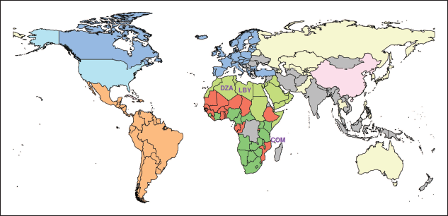
The other component of the network, on the right-hand side of Figure 1, is made out of three blocks. The block on the bottom contains all countries from the Middle East together with Northern African countries such as Libya, Tunisia, Egypt and Morocco. The middle block includes countries from Central and Western Africa. Finally, the upper block is composed of Southern African countries. The central block is well connected with both the northern and the southern blocks, mostly through countries that share borders, while the latter two blocks are instead only directly bridged by Sudan. As an additional note, we can observe that the two major components of the network are linked exclusively through France, that, while belonging to the European block, acts as a bridge between Africa and Europe itself. Finally, it is evident how transferring the group assignments to the world map in Figure 2 clearly reveals a general geographic proximity of countries belonging to the same community.

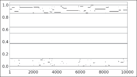
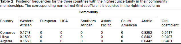
In addition to the detected block structure, we also investigate the uncertainty of the node allocation, using the Monte Carlo-based posterior samples. We therefore consider the last Gibbs sampling sequence after the algorithm has converged. More specifically, we take a look at the three countries with the lowest values of the normalized Gini coefficient calculated over the allocation frequencies, which in turn imply the highest uncertainty. These countries are Libya (LBY), Algeria (DZA) and Comoros (COM), which all belong to the Arabic block. The switching of communities exhibited by Libya throughout the posterior sampling is illustrated as an example in Figure 3. It shows how the sample for $U_{\mathit{Libya}}$ mostly appears within $[0.87,1]$ (the interval of the Arabic block) while also exhibiting some states where it is within $[0,0.13]$ (the interval of the Western African block). The posterior frequencies for Libya as well as for Comoros and Algeria with respect to the different groups are shown in Table 2, which also comprises the corresponding Gini coefficients. The table shows how all three countries have a substantial tendency to move to the Western African block. According to the fitted blockmodel, in 15% to 18% of the MCMC sample states the three countries are assigned to this block. Turning our attention to all other countries, we observe Gini coefficients which are close to one and thus exhibit only very little uncertainty in block membership. Altogether, this reveals how the estimated community structure appears to be quite strong.

Figure 3:

Posterior sample of the latent quantity U for Libya plotted against the MCMC states. Horizontal lines represent community boundaries

Table 2:

Posterior frequencies for the three countries with the highest uncertainty in their community memberships. The corresponding normalized Gini coefficient is depicted in the rightmost column

Community
Country	Western African	European	USA	Southern African	Asian/ Pacific	South American	Arabic	Gini coefficient
Comoros	0.1748	0	0	0	0	0	0.8252	0.9417
Libya	0.1598	0	0	0	0	0	0.8402	0.9467
Algeria	0.1558	0	0	0	0	0	0.8442	0.9481

5.2 Butterfly similarity network

The standard SBM as showcased in the previous section is suitable for modelling binary networks. As described in Section 2, this dataset is, however, comprised of similarity scores which lie in the interval [0,1.55]. While it would be possible to binarize the data, for example defining a threshold within the domain as cut-off, this would lead to considerable information loss. We therefore use the Poisson version of the stochastic blockmodel as defined in (3.2), taking advantage of the fact that this variant is suitable to treat multi-edged networks as well as binary ones. To fit this model, we discretized underlying similarity measures into count data through binning. More specifically, each similarity measure was multiplied by 100 and rounded to the nearest integer, resulting in natural values between 0 and 155. Estimation on the resulting multi-edged network was performed using the Variational EM approach developed by (Mariadassou et al.(2010); see also Daudin et al.(2008)) and implemented in the R software by Leger (2016). In this case, since we know that the real number of species is ten, we can simply use the same number of communities for the estimation. Figure 4 shows the results of the model fit compared with the partition of butterflies into species.

Figure 4:

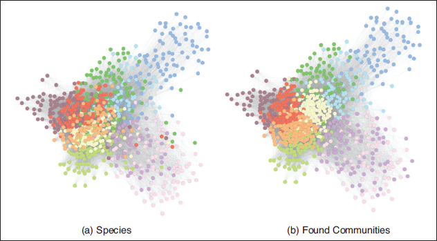
Comparison between ‘ground truth’ communities (species) and groups found by the Poisson stochastic blockmodel in a network of butterflies, with weighted edges representing the degree of visual similarity between them

At a first glance, we can see that the communities recovered mirror the real species relatively well. The most evident difference lies in the fact that two of the species (located towards the centre of the plot) are apparently really similar according to the utilized measure of visual similarity, and are therefore split up by the blockmodel. It is also interesting to note how communities found by the stochastic blockmodel seem to be visually clearer than ground truth ones. This is attributable to the fact that network visualization techniques and the clustering algorithm utilized are both based solely on the ties between the nodes, and thus tend to be more in accordance. The ground truth, on the other hand, is always given a priori, and can easily have outliers in terms of connectivity behaviour. In this specific case, visualization and blockmodelling are both based on the aforementioned measure of visual similarity between butterflies, while the ground truth communities are given by the classification of butterflies into species by biologists. This at least partially explains the discrepancy between the ground truth communities and the positioning of the nodes in the visualized graph. Despite this discrepancy, in general, the structure that was found does not appear to present major differences from the biological classification of the species. To quantify the goodness of the recovered block structure compared to the ‘ground truth’ communities, several measures are available (we refer to Jebabli et al.(2018) for a comprehensive survey). Here we opted for the Rand index, a measure of similarity between two data clusterings that can simply be described as the number of agreements in classifying pairs divided by the total number of pairs (Rand (1971)). The index takes values between $0$ and $1$ , and in this case it is equal to $0.91$ , indicating that, given two Butterflies chosen at random, the blockmodel is able to correctly identify if they belong to the same species or not 91% of times.

5.3 Email exchange network

This network of emails within a research institution exhibits a skewed degree distribution, as shown in Figure 5. This type of degree distribution is typical of real-world social networks, and leads the classical SBM to often only be able to find core-periphery type block structures, with nodes grouped mostly on the basis of degree similarity.

Figure 5:

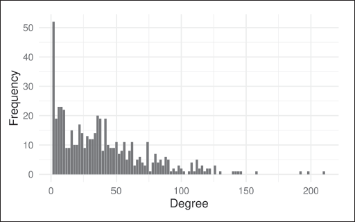
Empirical degree distribution of the email exchange network

As explained above, one way to circumvent this issue is to use degree correction. For this application, we therefore made use of the original version of the degree-corrected stochastic blockmodel as in (3.3) (Karrer and Newman (2011)). The results of the model fitting, together with the partitioning of the network into real departments, are visualized in Figure 6.

Figure 6:

Comparison between ‘ground truth’ communities (departments) and groups found by the degree-corrected stochastic blockmodel in a network of email exchanges within a large European research institution

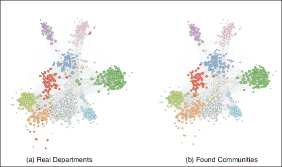
Looking at the plots, it is evident how the model with degree correction is able to recover the communities quite accurately. Comparing the partition discovered by the degree-corrected SBM with the actual departments, one small department (depicted towards the upper-centre of the figure) merges into another one close to it, and an additional block is therefore found at the bottom-centre of the plot, splitting the larger bottom department into two. Other than that, the structure found is remarkably similar to the partition induced by the departments, with some exceptions due to the existence of disconnected components within departments. In this case the Rand index is equal to 0.95, indicating a very high level of agreement among the partitions. For comparison purposes, we also fit a standard SBM to the same data, and computed the Rand index for the partition found with that as well. The resulting value of the index only amounts to 0.86, underlining the importance of applying degree correction in this case.

6 Conclusions

Mixture modelling can be extended to network data through stochastic blockmodels. Networks are rather complex structures, leading to computationally demanding estimation routines. Several algorithms specific for this class of problems have emerged over time, some of which are discussed in this article. We also provided an overview of different types of blockmodels by applying them to real-world network datasets. Among others, one of the models that we showcased is the degree-corrected stochastic blockmodel, which is particularly well suited for networks with a highly skewed degree structure.

Considering stochastic blockmodels (and community detection problems) as mixture models opens up a new avenue of extensions and novel models. Looking at the many model proposals in the field of mixture, ranging from mixing different distributions towards the mixture of experts, it is evident that these extensions can be brought forward in network modelling with mixtures as well. In fact, block-wise constant connectivity probabilities could be extended towards non-constant ones. Moreover, covariates could also be included. These extensions lie well beyond the scope of this article, but it is evident how the long history of mixture models, which started with Pearson (1894), has not come to an end, and extends promisingly in the realm of networks.

Appendix

Details on MCMC sampling scheme

Assuming 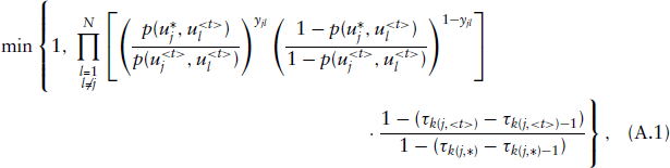${\mathbf{u}}^{<t>}=(u_1^{<t>},\dots ,u_N^{<t>})$ to be the current state of the Markov chain, we can update the $j$ th component as follows. At first, we set $u_l^{<t+1>}=u_l^{<t>}$ for all $l\ne j$ , while for component $u_j$ we draw a new potential state $u_j^{*}$ from a uniform proposal with regard to the domain $[0,1]\backslash [{\tau }_{k(j,<t>)-1},{\tau }_{k(j,<t>)})$ and with $[{\tau }_{k(j,<t>)-1},{\tau }_{k(j,<t>)})$ being the subinterval that includes $u_j^{<t>}$ . This leads to the acceptance probability

$$\begin{array}{r}\min \{1,{\displaystyle \prod _{\begin{array}{l}l=1\\ l\ne j\end{array}}^N\left[{\left(\frac{p\left(u_i^{\ast },u_l^{<t>}\right)}{p\left(u_j^{<t>},u_l^{<t>}\right)}\right)}^{y_{ii}}{\left(\frac{1-p\left(u_j^{\ast },u_l^{<t>}\right)}{1-p\left(u_j^{<t>},u_l^{<t>}\right)}\right)}^{1-y_i}\right]}\\ \cdot \frac{1-\left({\tau }_{k(j,<t>)}-{\tau }_{k(j,<t>)-1}\right)}{1-\left({\tau }_{k(j,\ast )}-{\tau }_{k(j,\ast )-1}\right)}\},\end{array}$$

(A.1)

where $[{\tau }_{k(j,*)-1},{\tau }_{k(j,*)})$ represents the subinterval which includes $u_j^{*}$ . If we accept the alteration, we set $u_j^{<t+1>}$ to the value $u_j^{*}$ , while in the event of rejection, we remain with the previous value $u_j^{<t>}$ . Running the Markov chain, we get a sampling sequence from which we derive a simulation-based estimate of the group mode, which concludes the E-step. It should be mentioned that, in the beginning, the number of Gibbs sampling states taken into account for approximating the posterior mode can be rather small, since the early model configurations are potentially far from the truth and thus already imply a deviating reallocation.

Label switching and non-identifiability

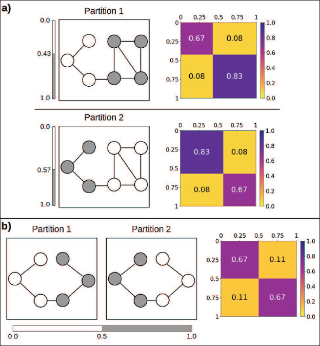
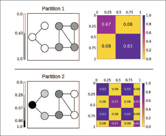
As has been extensively discussed in other works, approaching the conceptual formulation of mixture models by MCMC methods induces the label switching problem (see, for example, Stephens (2000)). This issue describes the invariance of the likelihood under relabelling of the mixture components. However, since in the proposed MCEM algorithm the model parameters are not part of the MCMC scheme but rather given as fixed based on the M-step, the label switching problem reduces to the exceptional case of symmetric parametrization. The two different situations can be exemplified by the configurations shown in Figure A.7.

Figure A.7

Simple examples to illustrate the label switching problem in SBMs expressed through graphon representation. a) Two plausible blockmodels for the same seven-node network which are specified by $U_i\lessgtr 3/7$ and $U_i\lessgtr 4/7$ , respectively (illustrated by node colors), and a corresponding step function $p(·,·)$ (depicted in the right column). Both models yield the same value for the likelihood and can be transferred into one another through label switching. b) Two potential partitions of a six-node network, each forming a blockmodel. The partitions can again be transferred into one another through label switching, but in this case they both refer to the same function $p(·,·)$ . Only b) poses a label switching problem for the proposed MCEM algorithm

In both of the depicted cases (a) and (b), the two respective models describe and capture the exact same structure of the respective given network. That means none of them is preferable, and it is thus unclear beforehand to which label ordering the algorithm will tend. Nevertheless, regarding the non-symmetric configuration in (a), we point out that our MCEM algorithm will remain in either one of the partitions once that has been reached. At the stage of convergence, fixing the model parameters based on the M-step will leave the partition unchanged in the MCMC-based E-step (if the Gibbs sampling sequence is chosen to be sufficiently large). This is because the posterior distribution of the allocations is not invariant to label switching when $p(·,·)$ is fixed. Only in the symmetric case (b) a label switching might occur, which here exclusively refers to the node assignments, since now not only the likelihood but also $p(·,·)$ is invariant to label switching. In the worst case, this might lead to a fuzzy estimate in the M-step representing an in-between state of the different partitions. However, we argue that the case of two (or more) groups exhibiting a very similar connectivity behaviour in regard to all other groups (and among themselves) is an extraordinary one, that is unlikely to occur in real-world applications.

Another issue similar to the label switching problem which is inherent in graphon models is that of non-identifiability. This issue consists in the fact that different arrangements of the function $p(·,·)$ represent the same model. More precisely, as has been shown by Diaconis and Janson (2008), two graphon functions $p(·,·)$ and $\tilde{p}(·,·)$ represent the same network-generating model if and only if there exist two measure preserving functions $\varphi ,\tilde{\varphi }:[0,1]\to [0,1]$ such that $p(\varphi (u),\varphi (v))=\tilde{p}(\tilde{\varphi }(u),\tilde{\varphi }(v))$ for almost every $(u,v)\in [0,1{]}^2$ . Accordingly, this also includes the label switching problem, although it only refers to the model specification (and not to the likewise affected node assignments). Another potential instance of the identifiablity issue in SBMs represented as graphon models lies in the splitting of groups. To illustrate that, we consider the two blockmodels in Figure A.8, which both capture the same structure in the given network.

Figure A.8

Simple example to illustrate the splitting of groups in SBMs expressed through graphon representation. The node colouring exhibits node assignments, with the corresponding graphon functions depicted on the right. Both of the models describe and capture the same block structure in the given network. Nevertheless, the upper model is preferable to the lower model with respect to the following three criteria: a monotonically non-decreasing marginal function, merging similarly behaving nodes, and parsimony in terms of the number of communities

As has been mentioned in Section 3.3, the identifiability issue can be resolved by assuming a monotonically non-decreasing marginal function. This condition only applies to the upper model representation. However, considering our MCEM algorithm, the E-step aims to merge nodes with similar connectivity behaviour and therefore naturally prevents the splitting of groups. In addition, the lower representation is that of a blockmodel with four groups, a number which, compared to the upper representation, appears to be unnecessarily inflated. We hence argue that the identifiability issue in regards to the splitting of groups is a matter of the applied blockmodel dimensionality and can be also prevented through an appropriate choice of the number of mixture components. We therefore avoid the additional constraint of a monotonically non-decreasing marginal function.