
Abstract
Fatal car crashes are the leading cause of death among teenagers in the USA. The Graduated Driver Licensing (GDL) programme is one effective policy for reducing the number of teen fatal car crashes. Our study focuses on the number of fatal car crashes in Michigan during 1990–2004 excluding 1997, when the GDL started. We use Poisson regression with spatially dependent random effects to model the county level teen car crash counts. We develop a measurement error model to account for the fact that the total teenage population in the county level is used as a proxy for the teenage driver population. To the best of our knowledge, there is no existing literature that considers adjustment for measurement error in an offset variable. Furthermore, limited work has addressed the measurement errors in the context of spatial data. In our modelling, a Berkson measurement error model with spatial random effects is applied to adjust for the error-prone offset variable in a Bayesian paradigm. The Bayesian Markov chain Monte Carlo (MCMC) sampling is implemented in rstan. To assess the consequence of adjusting for measurement error, we compared two models with and without adjustment for measurement error. We found the effect of a time indicator becomes less significant with the measurement-error adjustment. It leads to our conclusion that the reduced number of teen drivers can help explain, to some extent, the effectiveness of GDL.
Keywords
Introduction
Background
The main cause of death among teenagers in the USA is from motor vehicle accidents (Chen et al., 2014). In many developed countries, teen drivers have the highest crash involvement rate comparing to other driver age groups (Williams, 2003). Several approaches to reduce the number of fatal car accidents involving teenagers have been tested on and some are more successful than others. One effective policy that has been widely implemented is Graduated Driver Licensing (GDL; Shope, 2007). The three stages of GDL adopted by the state of Michigan in 1997 are as follows.
Stage I: Supervised learner period, novice teenagers are required to drive 20–60 h and hold the supervised license for a minimum length of time (6–12 months). Stage II: Intermediate stage of GDL, teenagers are allowed to drive independently with restrictions on driving at night and passengers. Stage III: Full-license stage of GDL, grants experienced teenager drivers full driving privileges without restrictions.
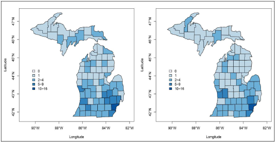
Figure 1 (reproduced plots and the original ones are in Chen et al. 2014) presents the teen driver fatal car crash counts before and after the implementation of GDL in the Michigan State. GDL became effective in Michigan in 1997. Similar to the findings in Chen et al. (2014), our data analysis results also show that GDL is effective. But our modelling is different than that in Chen et al. (2014). The key difference is that we distinguish the population of teenagers and the population of teen drivers, while they are considered approximately the same in Chen et al. (2014). More specifically, we embed a measurement error model on the offset variable in a Poisson regression model to reflect the difference between the aforementioned two populations.
Reproduced figure from Chen et al. (2014): County-level teen driver fatal car crash counts in Michigan in 1996 (left) and 2004 (right)
Reproduced figure from Chen et al. (2014): County-level teen driver fatal car crash counts in Michigan in 1996 (left) and 2004 (right)
We used the same data as that was analysed in Chen et al. (2014). Instead of following Chen et al.’s model, we use a Poisson regression to fit the data. The data are extracted from multiple sources, which are all publicly available. Previous studies showed that unemployment rate (Lenk, 1999), Rural–Urban Continuum index (Noland and Quddus, 2004) were associated with teenager-driver car crash counts. The data for unemployment rate in the state of Michigan were obtained from the US Bureau of Labor Statistics (
County-level teenager population data in the state of Michigan were extracted from the US Census database. Teenager population is used to adjust yearly counts of fatal teenager-driver crashes for variation in the size of the teenager population across counties, it can be incorporated as an offset term to the model. The population is widely considered as a surrogate for the number of licensed drivers and used for modelling the fatality rate in roadway traffic studies. This leads to a hierarchical model with measurement error, which will be discussed in following sections.
Because the recession of automobile industry in Michigan started from 2005 and this lead to changes in driving behaviour and the number of car crashes, we followed Chen et al. (2014) to collect the data seven years before (1990–1996) and after (1998–2004) the implementation of GDL. In Michigan, the most significant and recent urbanization period occurred during the auto-industrial boom that took place before the 1980s. Same as what Chen et al. (2014) did in their data analysis, we used the Rural–Urban Continuum Codes updated in 2003. This indeed does not reflect the true measurement of rurality during the study period 1990–2004. But given the code is updated only every 10 years, we consider it as an acceptable approximation.
Let
Measurement error in spatial modelling
There is a crucial yet implicit assumption in classical regression analysis: covariates are measured precisely. However, such an assumption is often violated in real life setting. Variables measured with error are commonly known as measurement error or errors-in-variables problem. There has been very rich literature in this area. For example, Carroll et al. (2006) provides comprehensive and systematic discussions as a classical textbook on this topic. Gustafson (2004) mainly focuses on Bayesian methods with emphasis on applications in epidemiological studies. Yi (2017) includes an update of recent developments for a variety of settings (e.g., event history data, correlated data, multi-state event data).
Relatively less literature addressed the measurement errors in the context of spatial data (e.g., Bernadinelli et al., 1997; Xia and Carlin, 1998; Li et al., 2009; Huque et al., 2016, 2014). All of the existing work focuses on error-prone covariates. To the best of our knowledge, no work has been conducted to adjust for the measurement error in an offset variable in combination with spatial random effects.
Conditional autoregressive (CAR) modelling (Cressie, 1993) is considered to account for the spatial dependence through random effects in multi-level models. Suppose we have random variables
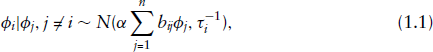
where
By Brook’s Lemma (Brook, 1964), the joint distribution of ϕ is:

where

The parameter
To explain the difference between the models in Chen et al. (2014) and the models in our data analysis. We will first introduce their models and then our models in the following subsections.
Models in Chen et al. (2014)
Chen et al. (2014) applied a log transformation to the adjusted observed yearly county-level fatality rates as their response variable, that is,

with the mean

Here
It is worth noting that the adjusted log fatality rates
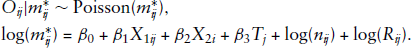
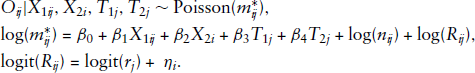
First, we introduce the naïve model without adjustment for the measurement error, that is,

where
In the previous model, we modelled the fatality rates in the Poisson regression by adding the offset term
Simply ignoring the measurement error in offset may cause biases in estimated regression coefficients. As shown in Chapter 3 of Zhang (2019), we can see the apparent discrepancy in parameter estimates between the models with and without adjustment for measurement error, particularly for regression coefficients of the predictors that are highly correlated with the number of licensed teen drivers.
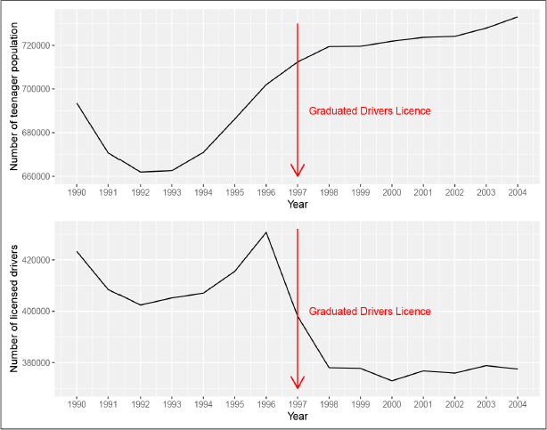
The total number of licensed teen drivers in Michigan is available at the state level from year 1990 to 2004 excluding 1997. For comparison, the state level teen population and the number of licensed teen drivers are plotted in Figure 2, which show that the teen population and the number of licensed teen drivers have opposite trends after the implementation of GDL.
State level teen population and number of licensed teen driver from year 1990 to 2004
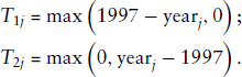
The actual offset variable should be
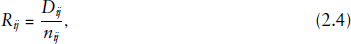
take the log of both sides of this equation:

Now embedding the measurement error model to account for the difference between
on of licensed teen driver is obtained at state level, it is natural to consider a Berkson type of measurement error model, that is,

where
Here is the summary of the differences between our proposed model and the one proposed in Chen et al. (2014). The key difference is the measurement error model we added to account for the difference between
We consider a Bayesian approach for model estimation. Details are presented in the following subsection.
Prior specification
In general, the prior distribution reflects the prior knowledge or information about the parameter of interest before collecting the data. If there is no such knowledge, then weakly-informative priors need to be assigned to the model parameters.
Prior for A CAR prior for Prior for Prior for spatial correlation

Stan/rstan for Bayesian MCMC sampling
The software Stan (Gelman et al., 2015) has been becoming popular due to its applicability to a wide variety of model settings. Stan differs from BUGS and JAGS in two primary ways. First, Stan is based on a new probabilistic programming language that is more flexible and expressive than the declarative graphical modelling languages underlying BUGS or JAGS, in ways such as declaring variables with types and supporting local variables and conditional statements. Second, the MCMC techniques in Stan are based on Hamiltonian Monte Carlo, a more efficient and robust sampler than Gibbs sampling or Metropolis-Hastings especially for complex models. In our data analysis, the Bayesian MCMC sampling is conducted by using an R pakcage ‘rstan’, which is an R interface for Stan. The source code for the data analysis can be found through
Data analysis
Model estimation
Given the complexity of our proposed models involving spatial random effects together with measurement error in the offset variable, we use Bayesian MCMC methods for model estimation.
The prior distributions for all parameters are listed in Section 2.3.1. We conduct the real data analysis under three different priors for the spatial correlation in the CAR model for the spatial random effects. We choose the values of the two hyperparameters to reflect the prior information on the spatial dependence.
Prior 1: Prior 2: Prior 3:
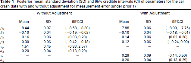
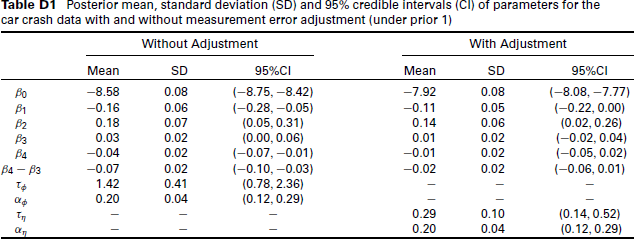
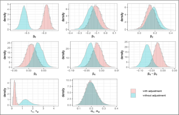
We ran multiple chains in all cases, and inspecting the results and the trace plots show no concern about convergence of the MCMC sampler. The posterior mean, standard deviation and 95% credible interval of each parameter in two models are summarized in Tables 1, A1 and A2 under three different priors for
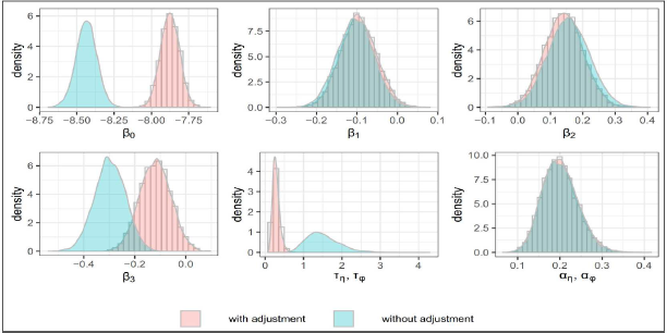
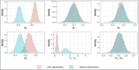
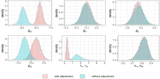
As indicated by the tables and plots, the posterior inferences for the regression coefficients of the unemployment rate and rurality are not affected by the adjustment of measurement error. While the posterior distributions of intercept and regression coefficient of time indicator have noticeable changes after adjusting for the measurement error. Moreover, the posterior distribution of the precision parameter
It is worth noting that the results are similar under three different prior choices for
Posterior mean, standard deviation (SD) and 95% credible intervals (CI) of parameters for the car crash data with and without adjustment for measurement error (under prior 1)
Posterior mean, standard deviation (SD) and 95% credible intervals (CI) of parameters for the car crash data with and without adjustment for measurement error (under prior 1)
Posterior distributions comparisons with and without measurement adjustment (under prior 1)
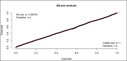
We check the fit of our proposed model by examining the randomized quantile residuals (Dunn and Smyth, 1996). In this section, only the results under the prior 2 for
Residuals are commonly used for statistical model checking. In normal linear regression model, QQ plots of residuals are commonly used as a model diagnostic tool. However, for a generalized linear model, the conventional diagnostics tool may fail as the distribution of residuals can be non-normal and heteroscedasticity even under the right model. A more general definition of residuals is proposed by Dunn and Smyth (1996), termed randomized quantile residuals (RQR). The key point is to add a randomization step when evaluating the fitted distribution function for a (discrete) response value to achieve continuous residuals. Basically, this is an extension from a continuous cumulative distribution function to a right-continuous distribution function. The randomized quantile residuals are (approximately) uniformly distributed over (0,1). ‘DHARMa’ (Ecology et al., 2019) is an R package for model diagnostics built upon the definition of RQR. In this section, we conduct residual diagnostics by using the package ‘DHARMa’ to create readily interpretable RQRs based on the 6 000 simulated (replicated) datasets of car crash counts. Figure 4 presents QQ plots based on quantile residuals from the model with adjustment for measurement error under moderate spatial dependence setting. The plot does not suggest obvious evidence for model-data misfit.
However, we acknowledge the limitations of this diagnostics method. First, it is in-sample prediction when we calculate the RQRs because the same data is used for model estimation and prediction. It is well known that this model check method can be overly optimistic. Second, in the original definition of RQR proposed in Dunn and Smyth (1996), the response variable has independent observations. Obviously this is not the case for the car crash counts in the motivating example.
QQ plot of DHARMa residuals with measurement error adjustment (under prior 2)
QQ plot of DHARMa residuals with measurement error adjustment (under prior 2)
In this study, we use Poisson regression model for analysing teen driver car crash counts with adjustment for errors in an offset variable. The model is clearly different than the previous work by Chen et al. (2014) for analysing the same data. We compare the results with a naïve model without adjustment for measurement error, that is, treating the population of teenagers as the same as the population of licensed teen drivers. We find that the inferences for the regression coefficients of
To the best knowledge of our knowledge, there is no existing literature about the adjustment of mismeasured offset in the context of spatial data. In our case, we construct the measurement error model with spatial random effects. In a similar fashion, this adjustment for errors in offset variables can also be applied to other models (e.g., Zero-Inflated Poisson model, Negative Binomial model) in spatial data case. In fact, zero-inflated Poisson models are also fitted to the real data example. Please refer to the Master's thesis of Zhang (2019) for details if interested.
WAIC values for the model with a single time covariate and two time covariates under five different CAR priors. Priors 1–3 are stated on page 9–10. Prior 4 is Uniform(
1,1) considered in Appendix B. Prior 5 is Uniform(0,1) considered in Appendix C
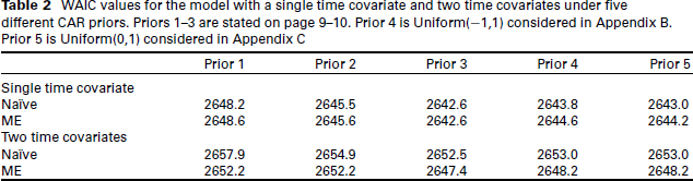
WAIC values for the model with a single time covariate and two time covariates under five different CAR priors. Priors 1–3 are stated on page 9–10. Prior 4 is Uniform(
1,1) considered in Appendix B. Prior 5 is Uniform(0,1) considered in Appendix C
Appendix
A Results under prior 2 and prior 3
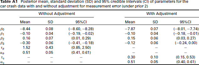
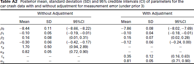
Posterior mean, standard deviation (SD) and 95% credible intervals (CI) of parameters for the car crash data with and without adjustment for measurement error (under prior 2)
Posterior distributions comparisons with and without measurement adjustment (under prior 2)
Posterior mean, standard deviation (SD) and 95% credible intervals (CI) of parameters for the car crash data with and without adjustment for measurement error (under prior 3)
Posterior distributions comparisons with and without measurement adjustment (under prior 3)
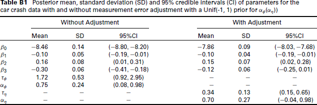
In this appendix, the posterior summary are based on the same model settings as model 2.3 and model 2.6 in Section 2.2 but with a Unif(
Posterior mean, standard deviation (SD) and 95% credible intervals (CI) of parameters for the car crash data with and without measurement error adjustment with a Unif(-1, 1) prior for
)
Posterior mean, standard deviation (SD) and 95% credible intervals (CI) of parameters for the car crash data with and without measurement error adjustment with a Unif(-1, 1) prior for
)
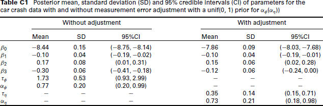
The following posterior summary statistics are from the same model settings as model 2.3 and model 2.6 in Sections 2.1 and 2.2. However, here we use a Unif(0, 1) prior for
Posterior mean, standard deviation (SD) and 95% credible intervals (CI) of parameters for the car crash data with and without measurement error adjustment with a unif(0, 1) prior for
)
D Results when using two time covariates
This section presents the results from the same model settings as model 2.3 and model 2.6 in Section 2.2 except for using two time terms (
Model without measurement error adjustment including two time terms:

Model with measurement error adjustment including two time terms:
Posterior mean, standard deviation (SD) and 95% credible intervals (CI) of parameters for the car crash data with and without measurement error adjustment (under prior 1)
Posterior distributions comparisons with and without measurement adjustment (under prior 1)
Footnotes
Acknowledgments
We would like to thank the comments/suggestions from the anonymous reviewers that have improved the presentation of the manuscript.
Declaration of Conflicting Interests
The authors declared no potential conflicts of interest with respect to the research, authorship and/or publication of this article.
Funding
The authors disclosed receipt of the following financial support for the research, authorship and/or publication of this article: The corresponding author's research was supported by a Discovery grant from the Natural Sciences and Engineering Research Council. The last co-author's research was supported by a grant from the National Cancer Institute (U01-CA057030), and also by a TRIPODS grant from the U.S. National Science Foundation (NSF CCF-1934904).