
Abstract
Longitudinal biomarkers such as patient-reported outcomes (PROs) and quality of life (QOL) are routinely collected in cancer clinical trials or other studies. Joint modelling of PRO/QOL and survival data can provide a comparative assessment of patient-reported changes in specific symptoms or global measures that correspond to changes in survival. Motivated by a head and neck cancer clinical trial, we develop a class of trajectory-based models for longitudinal and survival data with disease progression. Specifically, we propose a class of mixed effects regression models for longitudinal measures, a cure rate model for the disease progression time (
Keywords
Introduction
A patient-reported outcome (PRO) is any report of the status of a patient's health condition that comes directly from the patient, without interpretation of the patient's response by a clinician or anyone else (U.S. Food and Drug Administration Guidance for Industry, 2009). PROs can help identify symptoms or problems that may be missed during clinical queries, guide policy and health care delivery, and help patients choose between two equally efficacious therapies. Joint modelling of PRO and survival data can provide a comparative assessment of patient-reported changes in specific symptoms or global measures that correspond to changes in survival.
In joint modelling literature, there are usually a longitudinal component, a survival component and a dependence structure connecting those two components. There has been much work on joint modelling of one longitudinal measure and a survival measure, including Schluchter (1992), Hogan and Laird (1997), Law et al. (2002), Brown and Ibrahim (2003), Chen et al. (2004), Ibrahim et al. (2004), Brown et al. (2005), Chi and Ibrahim (2006), Chi and Ibrahim (2007), Ibrahim et al. (2010), Ye et al. (2008), Brown (2009), Rizopoulos (2012)), Pawitan and Self (1993), De Gruttola and Tu (1994), Lavalley and Degruttola (1996), De Gruttola and Tu (1994), Xu and Zeger (2001b), Xu and Zeger (2001a), Jacqmin-Gadda et al. (2010)) and (Proust-Lima et al. (2014)). (Tudur-Smith et al. (2016)) provided a recent review on joint modelling. In the recent development, multiple longitudinal processes and spline-based methods have been used in the joint modelling (Rizopoulos and Ghosh (2011)). Joint modelling has also been applied to more complex data structures such as competing risks data (Williamson et al., 2008; Elashoff et al., 2008; Huang et al., 2011; Li et al., 2012; Proust-Lima et al., 2016) and semi-competing risks data (Li and Su, 2017). In this article, we propose a mixed effects regression model for longitudinal measures, a cure rate model for the disease progression time (
Zhang et al. (2017)) developed a novel decomposition of DIC and LPML to assess the fit of the longitudinal and survival components of the joint model, separately. Based on this decomposition, they then proposed new Bayesian model assessment criteria, namely
The rest of the article is organized as follows. Section 2 gives a detailed description of the motivating longitudinal and survival data from a head and neck clinical cancer trial. In Section 3, we propose a mixed effects regression model for the longitudinal measure, a cure rate model for
Motivating longitudinal and survival data from a head and neck cancer clinical trial
The motivating study was an open-label, randomized, active-controlled phase III trial comparing the efficacy and safety of afatinib versus methotrexate in patients with recurrent/metastatic squamous carcinoma cancer of head and neck (HNSCC Machiels et al., 2015). Patients were treated on either afatinib or methotrexate, according to randomization, until the occurrence of disease progression or intolerable adverse events. Upon discontinuation of randomized treatment, a patient was free to take other anti-cancer therapies per protocol (except that patients discontinued methotrexate cannot start afatinib). It was reported that more than half of the patients who discontinued study medication started another anti-cancer treatment.
Graphical representation of the disease progression and survival data from the head and neck cancer clinical trial
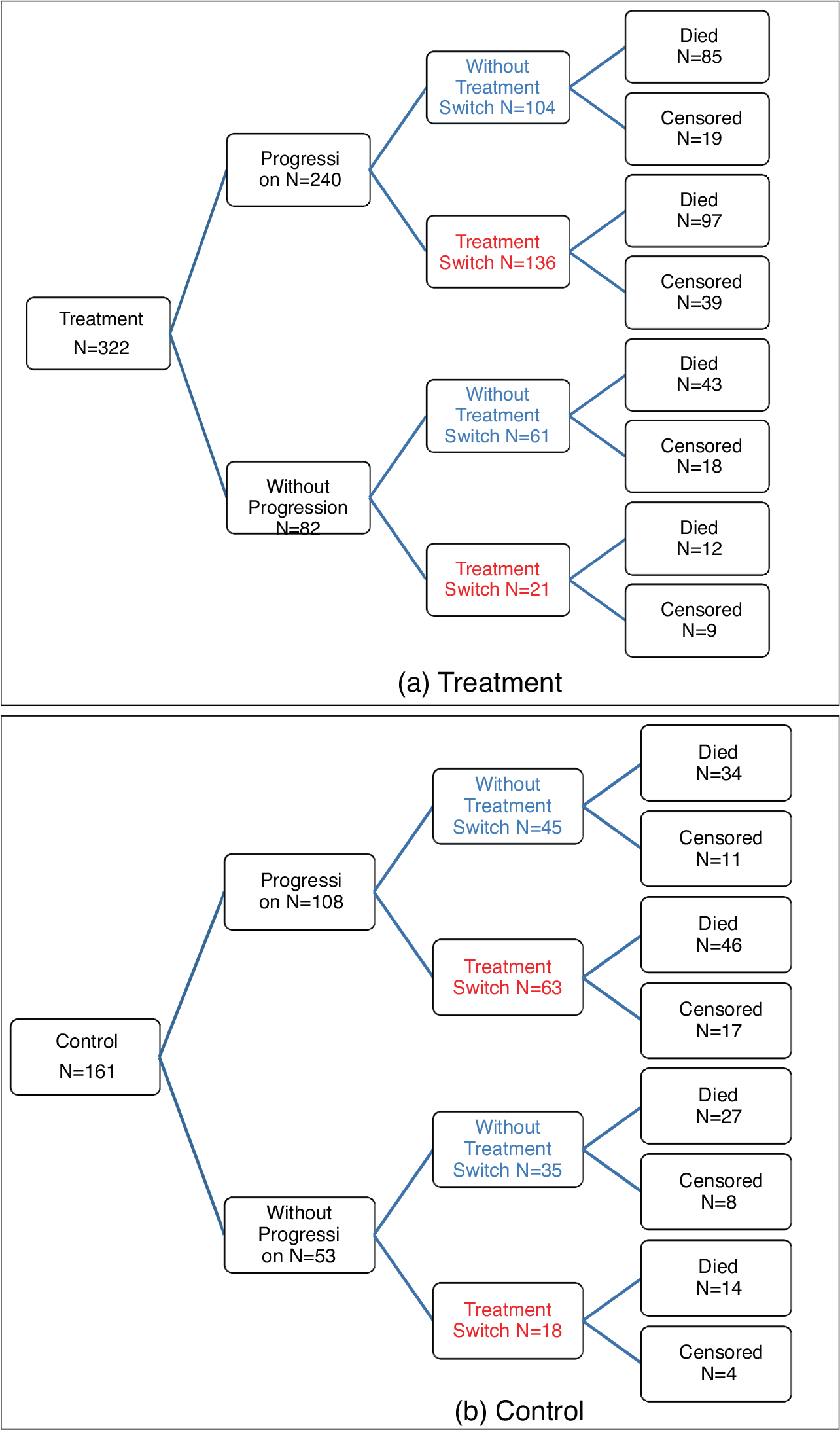
Graphical representation of the disease progression and survival data from the head and neck cancer clinical trial
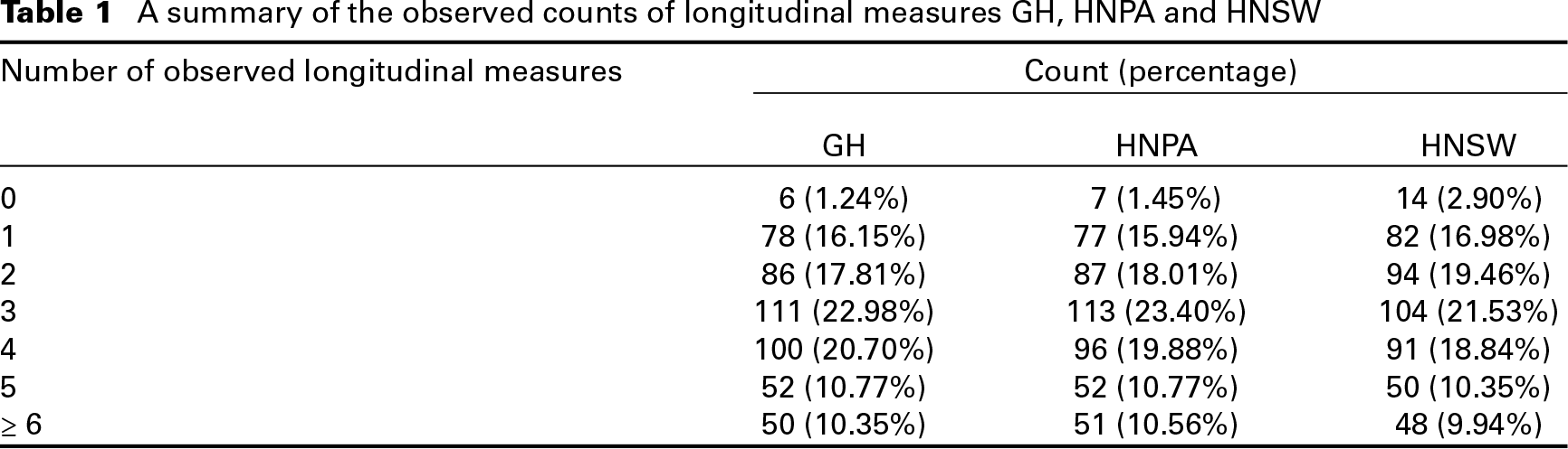
A summary of the observed counts of longitudinal measures GH, HNPA and HNSW
We consider the following baseline covariates: patients’ prior treatment with an epidermal growth factor receptor (EGFR)’targeted antibody, cetuximab (PEGFRA: 1 if and 0 if no), age more than 65 years (AGE: 1 if yes and 0 if no), gender (SEX: male/female), prior treatment with plantinum-based chemotherapy and radiotherapy (PCRTDC: 1 if yes and 0 if no), primary tumour site (TMSITED01: 1 if oral cavity, oropharynx, hypopharynx, larynx and 0 if others), metastatic sites of lymph node (METLOC2: 1 if yes and 0 if no), metastatic sites of lung (METLOC3: 1 if yes and 0 if no), liver (METLOC4: 1 if yes and 0 if no), or bone (METLOC5: 1 if yes and 0 if no), Eastern Cooperative Oncology Group (ECOG) performance status at baseline (ECOG: 0/1) and BSDTARG (Baseline target lesion: mm). We exclude two patients from the analysis because of missing BSDTARG measures.
Median survival time in days and its 95% confidence interval are 434 and (386, 470), median switch time, and its 95% confidence interval are 166 and (147, 190), and median progression time and its 95% confidence interval are 84 and (81, 86).
Let
Longitudinal component of the joint model
We first assume a mixed effects regression model for the longitudinal measure 
where 
where 
where
We note that in (3.1), if 
and a reparametrized version of (3.1) is written as

Then for any values of
Let 
where 
and a Cox-type model when 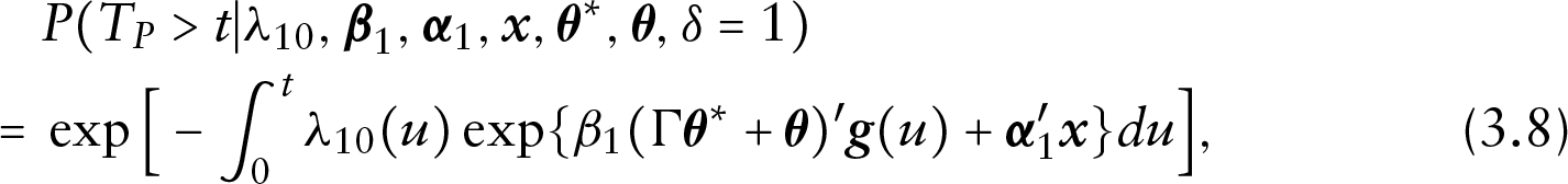
where 
where
We assume a time-varying covariates Cox model for 
where
Suppose that there are
Write 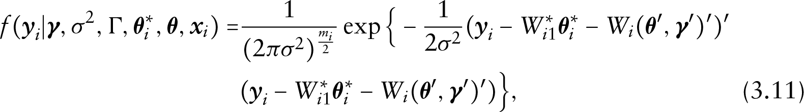
where
Using (3.2), the density of 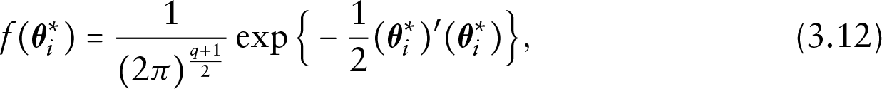
for
Based on the definition of
Define the survival function for
Under the proposed cure rate and time-varying covariates model, the observed data can be divided into four groups of observations. We derive the likelihood function for each of the four groups as follows.


Prior and posterior distributions
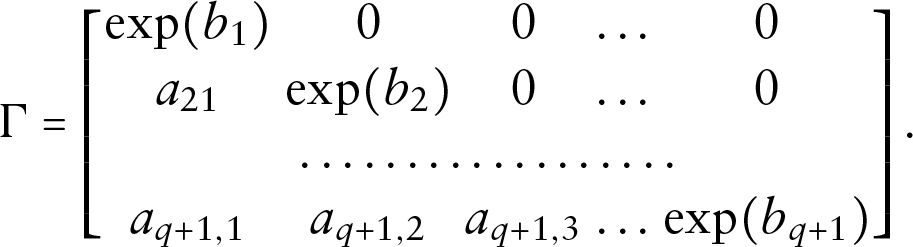
In (3.8) and (3.10), we assume a piecewise constant hazard function for 
where
Let 
Let 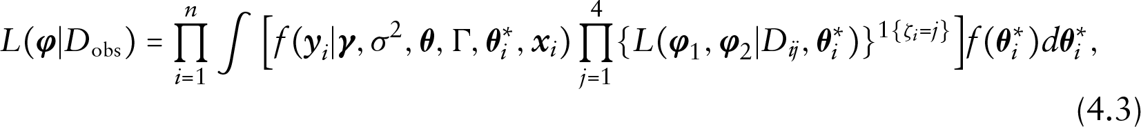
where 
where

To ease exposition, we present the computational algorithm only for 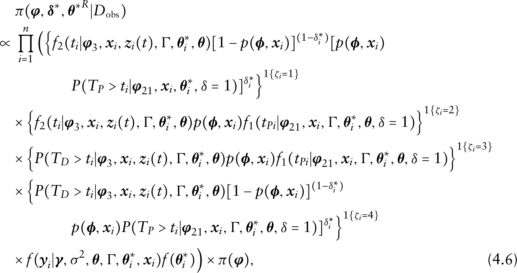
where
Although an analytical evaluation of the posterior distribution in (4.4) is not possible, a convenient Gibbs sampling algorithm can be developed to sample from the augmented posterior distribution in (4.6). Specifically, we sample from the following full conditional distributions in turn: (i)
Let
Define the joint distribution of of 
and the marginal distribution 
Based on the joint distributions, define the following conditional distributions:
The deviance information criterion (DIC; Spiegelhalter et al. (2002)) for the model is defined as

where
To assess the fit of the longitudinal component of the model and the fit of each survival component, we decompose DIC into three parts:

where
Write
When we fit the survival data alone, assuming 
where 
Similarly, denote

where 
where 
and
As pointed out in Zhang et al. (2017), when the penalty for the additional parameters in the overall survival model (3.10) or the time to progression model (3.8) outweighs the gain of the fit in the respective survival component,
In this subsection, we first establish the conditional predictive ordinate (CPO) identity which will lead to the decomposition of CPO. CPO (Geisser and Eddy, 1979; Chen et al., 2000; Zhang et al., 2017) for the 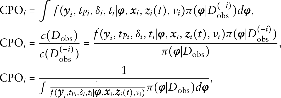
where
Let 
We also observe that 
where
Let 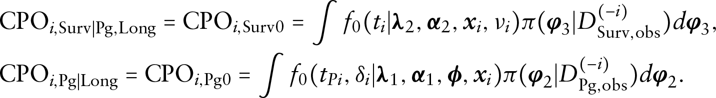
From Section S.2 in the supplementary materials, we have the following identities for 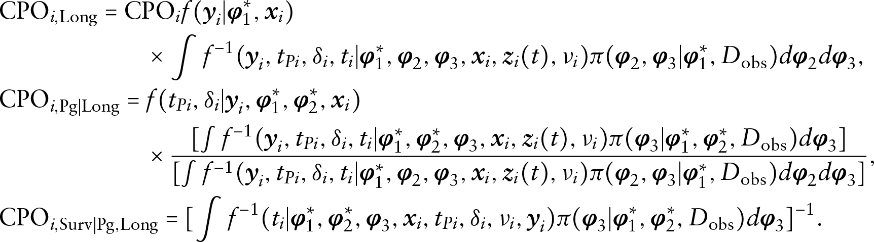
The logarithm of the pseudo-marginal likelihood (LPML; Ibrahim et al., 2001) is defined as
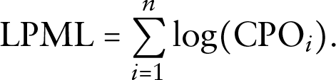
Then LPML can be decomposed as

where
Under the same assumptions for the calculation of 
Now, let 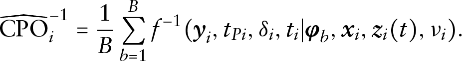
Next, fix 
Next, fix 
Finally,

Similarly,
Next, fix 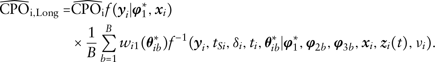
Next, fix 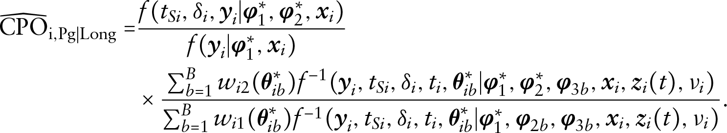
Finally,
Due to the computational difficulty of the optimal weight functions, another possible choice is
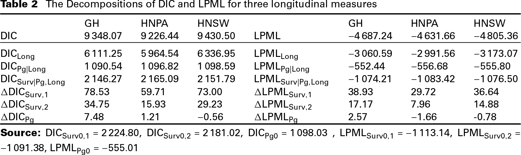
We apply our proposed method in Section 3 to analyse the head and neck cancer data introduced in Section 2. Out of the total 483 patients, we exclude two patients from the analysis because of missing BSDTARG0 measures. We are interested in identifying which of the three patient-reported measures: GH, HNPA and HNSW contributes most to the model fit of the survival data. Each of GH, HNPA and HNSW was measured on a continuous scale from 0 to 100. Following Ibrahim et al. (2001), we apply transformation to the original longitudinal measures:
We used DIC and LPML under the survival model alone for overall survival and the cure rate model alone for time to progression to determine
Diagram of the decompositions of DIC and LPML for the disease progression and survival data jointly with GH
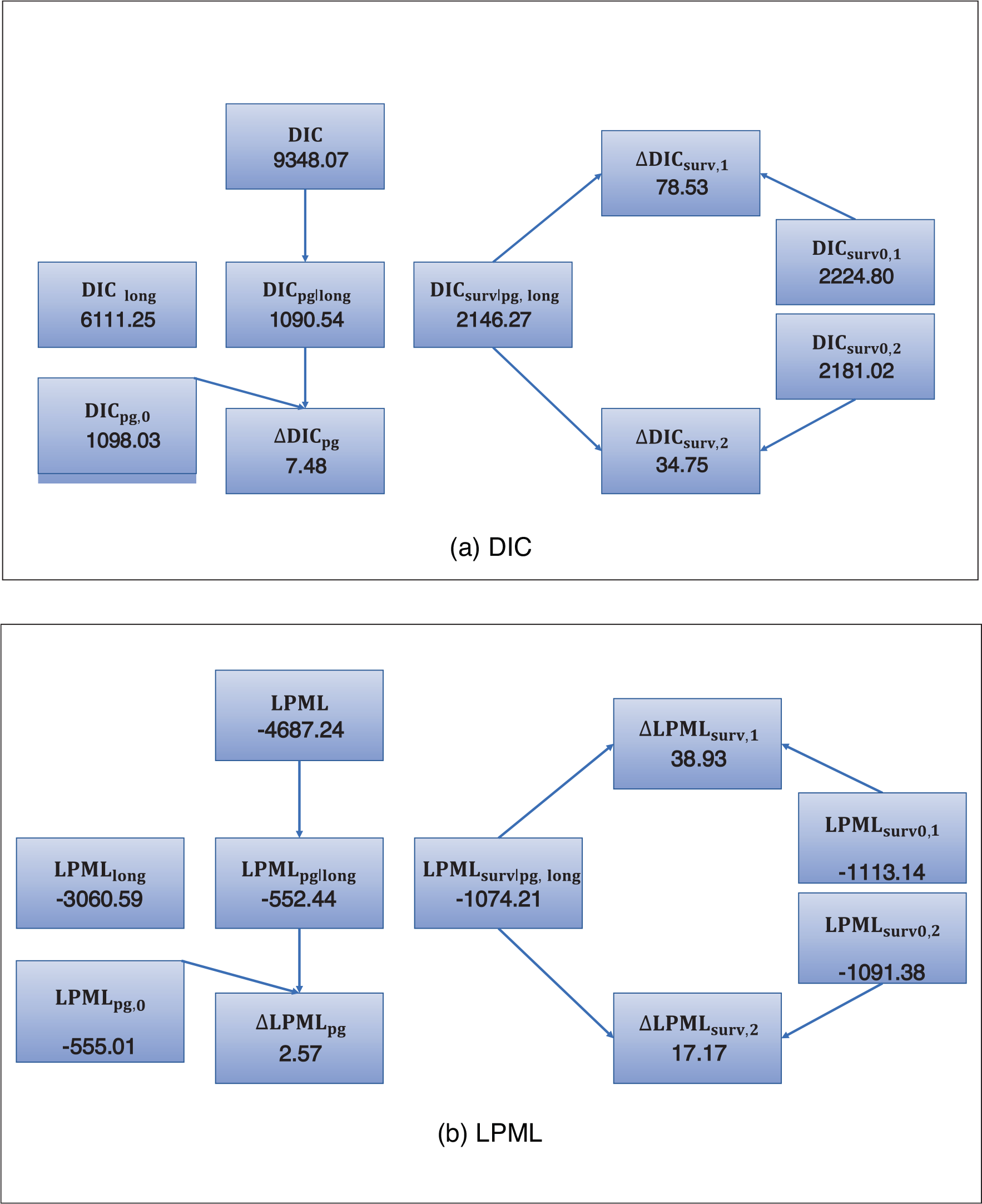
Diagram of the decompositions of DIC and LPML for the disease progression and survival data jointly with GH
Larger values of
The Decompositions of DIC and LPML for three longitudinal measures
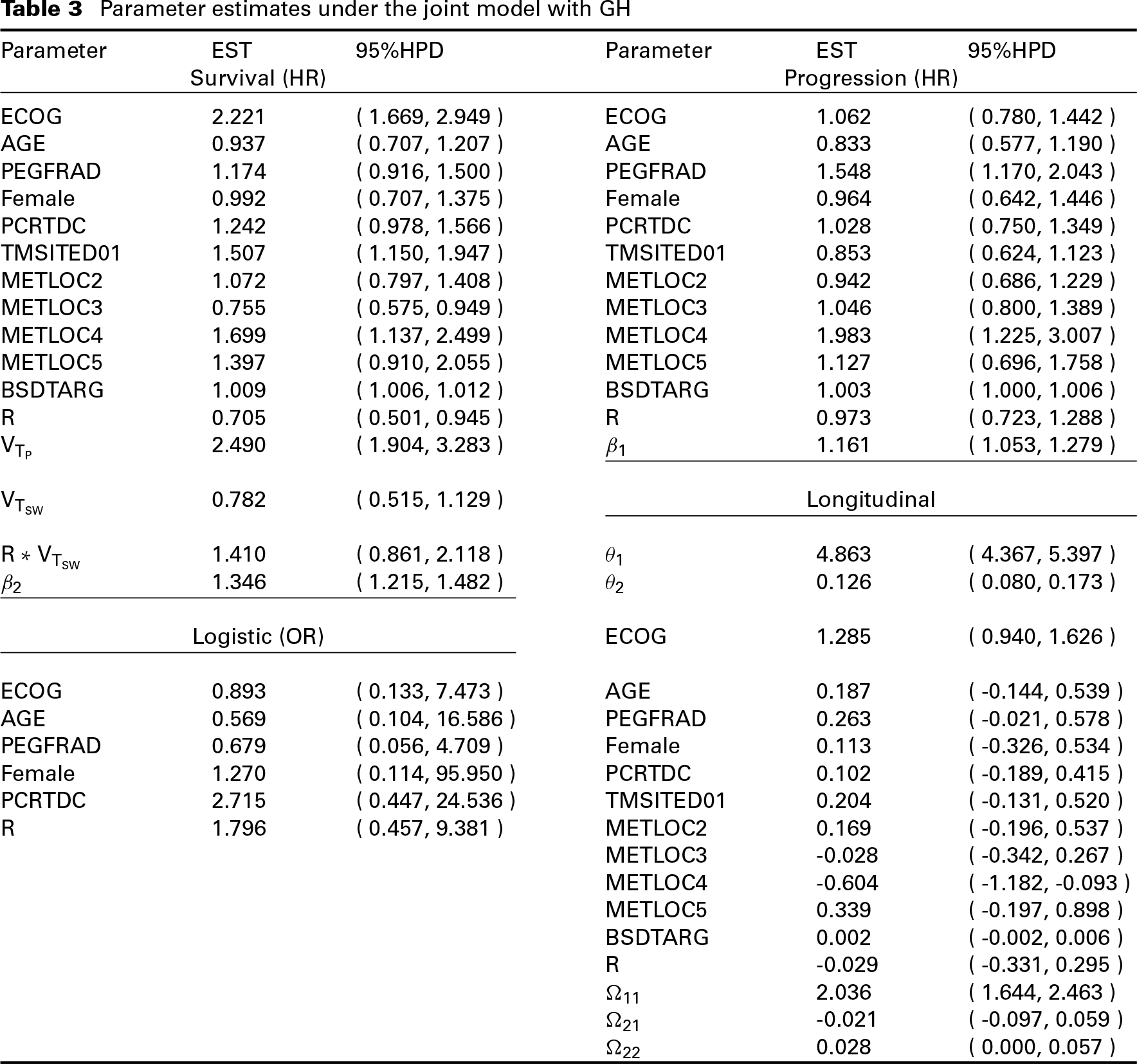
Parameter estimates under the joint model with GH
In all the Bayesian computations, we used 5 000 MCMC samples, which were taken from every third iteration, after a burn-in of 1 500 iterations for each model to compute all posterior estimates, including posterior means, posterior SDs, 95% HPD intervals, DIC and LPML. The convergence of the MCMC sampling algorithm was checked using several diagnostic procedures discussed in (Chen et al., 2000). The trace and autocorrelation plots of MCMC chains for the model parameters are shown in Figures S.1 to S.18. We see from these figures that the autocorrelations disappear even after lag 2 for some parameters and after lag 20 for most of the parameters. These trace and autocorrelation plots show good convergence and mixing of these MCMC chains. The HPD intervals were computed via the Monte Carlo method developed by (Chen and Shao, 1999). Computer code was written for the FORTRAN 95 compiler, and we used IMSL subroutines with double precision accuracy. The FORTRAN code is available from the authors upon request. In addition, an R interface of our Fortran code is developed, which can be downloaded from the journal website (
In this article, we proposed a class of mixed effects regression models for longitudinal measures, a cure rate model for the disease progression time and a time-varying covariates model for the overall survival. In Section 5, we carried out a Bayesian analysis of the head and neck cancer data using the computational algorithm discussed in Section 4.2. To examine the empirical performance of the posterior estimates under the proposed joint model, we conducted a simulation study. The design and results of the simulation study are presented in Section S.3 of the supplementary materials. As shown in Table S.1, the posterior estimates are close to the true values for almost all of the parameters except for
Within the semi-competing risk setting, we developed the decompositions of DIC and LPML to determine which PRO is most associated with the survival outcome. As discussed in Section 4.3, the DIC and DIC decompositions require a numerical approximation of an integral over random effects
Footnotes
Acknowledgments
This work was done when Dr Zhang was at University of Connecticut and when Dr Cong was at Boehringer Ingelheim (China) Investment Co. Ltd, Shanghai, China. We would like to thank the guest editors and two anonymous reviewers for their very helpful and constructive comments, which have led to a much improved version of the article.
Declaration of conflicting interests
The authors declared no potential conflicts of interest with respect to the research, authorship and/or publication of this article.
Funding
Dr M.-H. Chen's research was partially supported by NIH grants #GM 70335 and #CA 74015.
Supplementary materials
The supplementary materials, which include Section S.1 The Full Conditional Posterior Distributions, Section S.2 Results and Formulas, Section S.3 A Simulation Study, Tables S.1 to S.7 and Figures S.1 to S.18, can be found through the link: