
Abstract
Dropout is a common complication in longitudinal studies, especially since the distinction between missing not at random (MNAR) and missing at random (MAR) dropout is intractable. Consequently, one starts with an analysis that is valid under MAR and then performs a sensitivity analysis by considering MNAR departures from it. To this end, specific classes of joint models, such as pattern-mixture models (PMMs) and selection models (SeMs), have been proposed. On the contrary, shared-parameter models (SPMs) have received less attention, possibly because they do not embody a characterization of MAR. A few approaches to achieve MAR in SPMs exist, but are difficult to implement in existing software. In this article, we focus on SPMs for incomplete longitudinal and time-to-dropout data and propose an alternative characterization of MAR by exploiting the conditional independence assumption, under which outcome and missingness are independent given a set of random effects. By doing so, the censoring distribution can be utilized to cover a wide range of assumptions for the missing data mechanism on the subject-specific level. This approach offers substantial advantages over its counterparts and can be easily implemented in existing software. More specifically, it offers flexibility over the assumption for the missing data generating mechanism that governs dropout by allowing subject-specific perturbations of the censoring distribution, whereas in PMMs and SeMs dropout is considered MNAR strictly.
Introduction
Follow-up studies that include human subjects are known to be highly susceptible to dropout. The extent to which dropout will complicate the subsequent analysis depends on how the missingness is associated with the observed and unobserved longitudinal outcomes. According to the taxonomy introduced by (Rubin (1976)) and (Little and Rubin (2002)), this may happen according to three distinct missing data mechanisms: missing completely at random (MCAR), missing at random (MAR) and missing not at random (MNAR). Under MCAR, the missingness depends on neither observed nor unobserved outcomes. If the missingness is independent of the unobserved outcomes after conditioning on the observed outcomes, then the missing data mechanism is considered to be MAR. Conversely, under MNAR, conditioning on the observed outcomes cannot disentangle the dependence between the missingness process and the unobserved outcomes.
What separates MNAR from its counterparts in applied practice, though, is the concept of ignorability. That is under the (Bayesian) likelihood framework, one does not need to consider a model for the missingness process and hence ‘ignore’ it. Ignorability holds under the assumption that the process that generates the missing data is MAR and that the missingness and measurement processes depend on independent sets of parameters. While the innate convenience of ignorability popularized MAR models, one needs to consider if such an assumption holds carefully. That is especially the case since the distinction between MAR and MNAR is intractable as for every MNAR model, there exists a MAR counterpart with the same fit to the observed data (Molenberghs et al.(2008)Molenberghs, Beunckens, Sotto, and Kenward). Hence, one should start with an analysis that is valid under MAR and then perform a sensitivity analysis considering plausible MNAR departures from it.
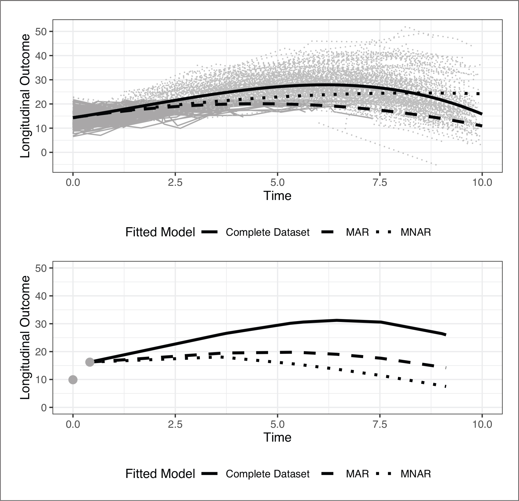
To showcase the importance of such sensitivity analysis, consider the illustrative example in Figure 1 which is based on simulated data. The data were simulated assuming a joint model for longitudinal and survival data. To mimic MAR missingness, censoring was based on the value of previous repeated measurements, and therefore the missing longitudinal trajectories (depicted with dotted grey) consist of the subjects that fulfilled the MAR criterion or experienced the event. We then fitted a model to the complete data, whereas for the incomplete data we fitted an MAR and an MNAR model. All three models resulted in different fits to the data, which consequently lead to different subject-specific predictions as shown in the lower panel of Figure 1. Therefore, sensitivity analysis is necessary to be able to investigate the robustness of the model and the plausibility of the assumptions concerning the mechanism that generated the missing data.
To this purpose, three well-established general frameworks exist, distinguished by their approach in factoring the joint distribution of the outcome and missingness processes to conditionally independent components. In a pattern-mixture model (PMM), the joint distribution is expressed as the product of the marginal distribution of the missingness process and the conditional distribution of the outcome given the missingness process. Contrariwise, in a selection model (SeM), the joint distribution is expressed as the product of the marginal distribution of the outcome and the conditional distribution of the missingness process given the outcome. Alternatively, in a shared-parameter model (SPM), the outcome and the missingness processes are assumed to be driven by a set of unobserved variables, the so-called random effects. The use of latent variables gives rise to the conditional independence assumption under which the outcome and the missingness processes are independent, given the set of random effects.
The SeM framework naturally encompasses MAR, while (Molenberghs et al.(1998)Molenberghs, Michiels, Kenward, and Diggle) provided a characterization of MAR under the PMM setting, specifically for the case of longitudinal data with dropout. As a result, sensitivity analysis is well-developed in the SeM and the PMM frameworks (Molenberghs and Vereke (2005); Molenberghs and Kenward (2007)), whereas the SPM has received less attention. More specifically, (Creemers et al.(2011)Creemers, Hens, Aerts, Molenberghs, Verbeke, and Kenward) provided a characterization of MAR for the SPM case by introducing the general SPM (GSPM) and then proposed a sensitivity analysis approach utilizing this framework (Creemers et al.(2010)Creemers, Hens, Aerts, Molenberghs, Verbeke, and Kenward). Later, (Njagi et al.(2014)Njagi, Molenberghs, Kenward, Verbeke, and Rizopoulos) proposed a characterization of MAR for the case of SPMs for longitudinal and time-to-event data under the GSPM.
In this article, we introduce an alternative characterization of MAR in SPMs for longitudinal and time-to-event data by exploiting the conditional independence assumption and utilizing the censoring distribution. By doing so, we cover a wide range of assumptions for the missing data mechanism on the subject-specific level. Previous work on the topic focused on the GSPM, which includes potentially a broad set of random effects. Here, we focus on the standard SPM (Wu and Carroll (1988); Wu and Bailey (1988); Wu and Bailey (1989); Hogan and Laird (1997); Hogan and Laird (1998)), a particular case of the GSPM, that is most commonly encountered in practice. The benefit of doing so is that our approach is intuitively appealing and can be easily implemented in existing software. Furthermore, it allows for subject-specific perturbations of the censoring distribution, concerning the missing data generating mechanism, whereas in PMMs and SeMs dropout is considered MNAR strictly.
The rest of the article is structured as follows. In Section 2, we propose an alternative characterization of MAR for the SPM model. In Section 3, we discuss its estimation under the Bayesian framework. In Section 4, we illustrate with an application how the SPM can be used for sensitivity analysis with existing software. In Section 5, we present a simulation study to assess the behaviour of the proposed sensitivity analysis under different scenarios with respect to the amount of MAR and MNAR missingness. Discussion follows in Section 6.
Illustrative Example: (Upper panel) observed longitudinal trajectories (black lines), missing longitudinal trajectories (grey), and fitted models using complete data and using incomplete data under MAR and MNAR. (Lower Panel) observed longitudinal measurements of a new subject and subject-specific predictions based on the three different models
Illustrative Example: (Upper panel) observed longitudinal trajectories (black lines), missing longitudinal trajectories (grey), and fitted models using complete data and using incomplete data under MAR and MNAR. (Lower Panel) observed longitudinal measurements of a new subject and subject-specific predictions based on the three different models
For each subject
What differentiates dropout from censoring in such a setting pertains to the causes of leaving the study. As an example, consider the case of a study, with death as the main outcome and where a longitudinal outcome is also planned to be recorded for a time period. The planned longitudinal outcome measurements will be missing for both the subjects that died during the study but also for subjects that dropped out from the study due to any other reason (e.g., they moved to another country). Depending on the information available and the research setting, one may define death as the only cause of dropout and assume all the other reasons are non-informative and therefore record them as censoring. In the case where no information is available for the cause of dropout, then one would consider only those who completed the study as censored.
Under this framework and with covariate vectors suppressed from the notation, the shared parameter model can be specified as follows:

where

which brings to light the core assumption of conditional independence in SPMs, under which the measurement and the dropout processes are independent conditional on the random effects. Note that the conditional independence assumption commonly does not imply independence of the censoring and the measurement processes. More specifically, in the general case, censoring is allowed to depend on the measurement process. Note that the conditional independence assumption may be extended to allow for independence of the censoring and the measurement processes as well. Finally, the assumption of non-informative censoring, which we discuss later, may be used to relax both these assumptions and allow for independence between the censoring and measurement processes.
Model (2.2) is a conventional SPM for longitudinal and time-to-event data. The term conventional here is in reference to the GSPM framework in the sense that a single common underlying random effects structure is used instead of multiple random effects structures. Another important note for model (2.1) is that by definition it allows for dependence between the dropout process

which, in other words, means that the censoring process no longer depends on the random effects and the missing observations. It should be noted that the assumption of non-informative censoring, while commonly applicable, may not always be a reasonable choice depending on the setting under study. Nevertheless, it is a necessary condition for achieving an MAR characterization in SPMs without introducing more latent variables as in (Creemers et al.(2011)Creemers, Hens, Aerts, Molenberghs, Verbeke, and Kenward).
Note that by definition, a subject may either be classified as a dropout or as censored and never both. This means that the decomposition of the joint density as described in (2.3) is, on a subject-specific level, further decomposed to the following:
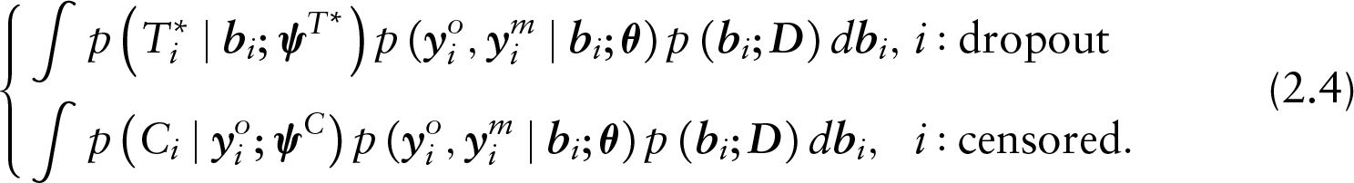
The decomposition in (2.4) reveals that SPMs encompass MAR on the subject-specific level. That is for a subject who dropped out from the study, the model is MNAR because both the dropout,
Estimation of the SPM under MAR follows from the conventional joint model for longitudinal and time-to-event data, which exploits the decomposition of the full joint-likelihood function to conditional independent components given the random effects. More specifically, the likelihood contribution of the

The form of the conditional densities depends then on the model specification of each component. Let the risk of dropout for subject
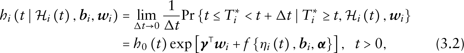
where
since based on the assumption of non-informative censoring, it cannot depend on the missing observations and the random effects.
The probability of not dropping out from the study can then be obtained by the following:
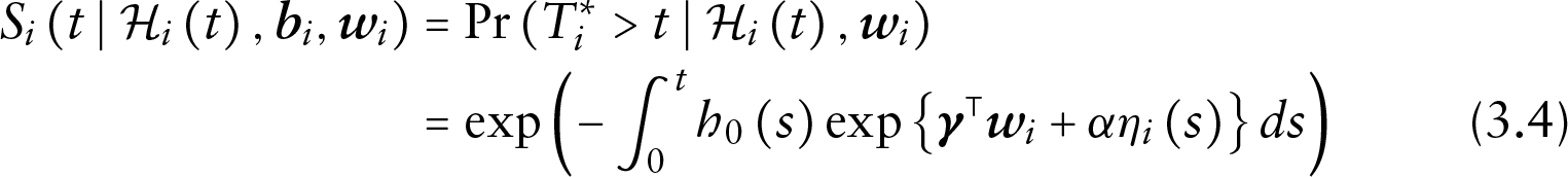
which means that unlike the instantaneous risk of dropout, the probability of remaining in the study depends on the whole true underlying subject-specific trajectory up to time
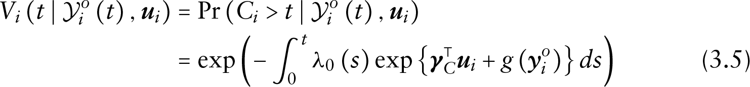
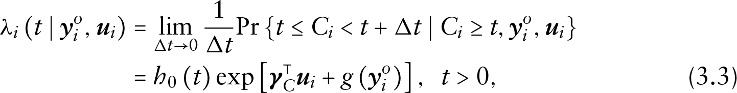
omitting the conditioning on missing values and the random effects due to the non-informative censoring assumption. Finally, to distinguish between censored subjects and dropouts, let
Under these assumptions and suppressing covariates

while the conditional density of the censoring process is given by the following:

Depending on the dropout and censoring status of the
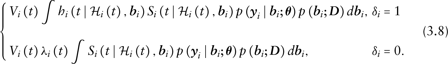
Under (3.8), the model is MNAR for both uncensored and censored subjects. The latter is because even for censored subjects, the term

which due to ignorability further reduces to the following:

an MAR model for the observed longitudinal measurements. The transition from equation (3.9) to (3.10) holds due to the fact that the instantaneous risk to be censored
As far as the true underlying longitudinal trajectory is concerned, let
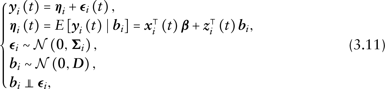
where the true longitudinal trajectory
The conditional density for the longitudinal responses is then given by the following:

with

Under the Bayesian framework, estimation of the parameters of the SPM is achieved using Markov chain Monte Carlo (MCMC) algorithms. Let

The computation of the integrals involved in
with

In the above specification,
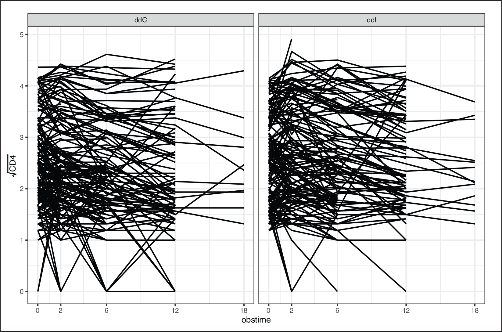
Observed longitudinal trajectories of
by treatment arm
Observed longitudinal trajectories of
by treatment arm
As an illustrative case study, we will use data from a randomized clinical trial designed to compare the efficacy and safety of Didanosine (ddI) versus Zalcitabine (ddC) in HIV patients (Abrams et al.(1994)Abrams, Goldman, Launer, Korvick, Neaton, Crane, Grodesky, Wakefield, Muth, Kornegay, Cohn, Harris, Luskin-Hawk, Markowitz, Sampson, Thompson, and Deyton; Goldman et al.(1996)Goldman, Carlin, Crane, Launer, Korvick, Deyton, and D.). In total, 467 advanced HIV patients were included in the study and were randomized to ddI (230; 49.2%) or ddC (237; 50.8%). The primary goal of the trial was to compare survival between the two treatment arms, while a secondary goal of the study was to investigate the association between CD4 cell count (a marker for the strength of the immune system) and the risk of death. For the latter goal, measurements of the CD4 cell count were recorded at scheduled visits at baseline, 2, 6, 12 and 18 months after the start of the study. Figure 2 shows the observed trajectories of the square root CD4 cell count. Until the end of the study, 184 (39.4%) died while only 1 405 (60.1%) out of the 2 335 planned visits were recorded, leading to 930 (39.9%) missing observations. In total, only 24(5.1%) patients were present for all five planned visits, 382(81.8%) dropped out from the study due to death or other reasons, and 61(13.0%) missed at least one planned visit without dropping out though from the remainder of the study. Table 1 shows the number of available measurements per dropout pattern per treatment arm, excluding the 61 cases of intermittent missingness.
Number of observed CD4 measurements per dropout pattern and per treatment arm. ‘OXXXX’ denotes a dropout pattern where only the first planned measurement was obtained (denoted with ‘O’) while the rest were not (denoted with ‘X’), whereas ‘OOOOO’ denotes a pattern for a completer (all planned measurements were obtained)
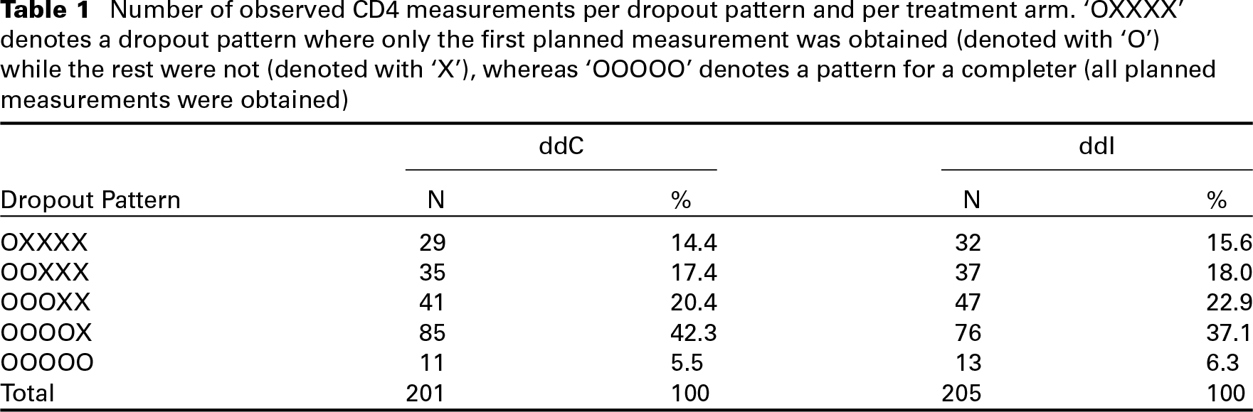
We observe that dropout rates are similar between the treatment groups, the closer we look at the beginning of the study, but they slightly start to deviate towards the end of the study. Nevertheless, it is not possible to distinguish if the missing data are missing completely at random, MAR or MNAR. This highlights the importance of being able to explore different scenarios with respect to missing data in the SPM framework via sensitivity analysis.
To model the longitudinal measurements of CD4 cell count, we used a linear mixed-effects model with an interaction between time and ddI in the fixed-effects structure. We also used random intercepts and random slopes to allow for subject-specific deviations. The square root of the CD4 cell count was used in order to meet the normality and homoscedasticity assumptions of the model, which is defined as follows:

where
For the time-to-dropout 
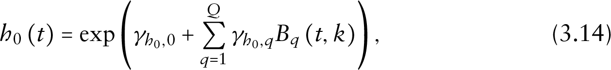
where the baseline hazard
These two sub models define the MNAR joint model for the CD4 cell count and the dropout. We then assumed two different scenarios with respect to the cause of dropout. Under Scenario 1, we assume no information concerning the cause of dropout, which means we treat dropout due to death or any other reason the same. Contrariwise in Scenario 2, we consider as dropouts only the subjects who died during the study. Finally, to achieve MAR, we assume that all the subjects are censored instead of dropping out. As shown in Section 3, this reduces the model to the mixed-effects sub model, which is considered MAR. All models were fitted using
Posterior means (standard errors) for an MAR and MNAR analyses
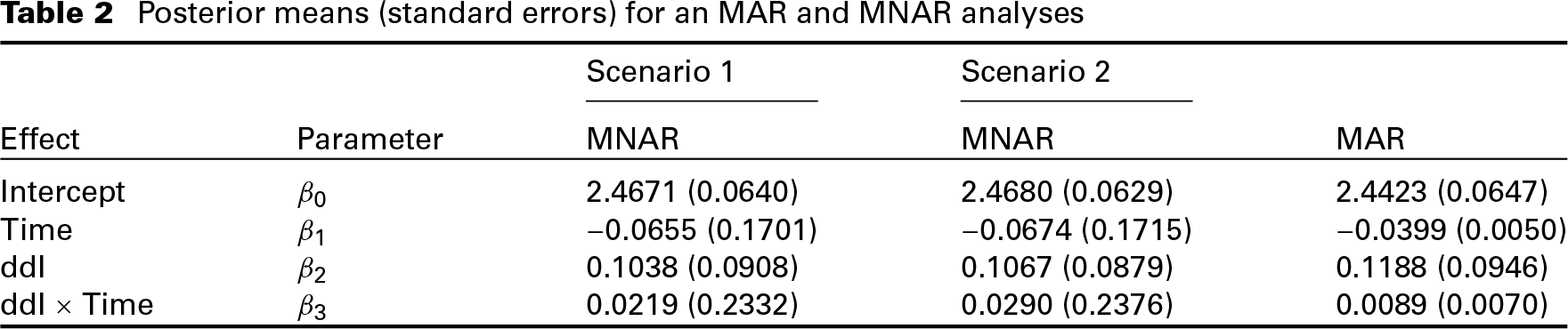
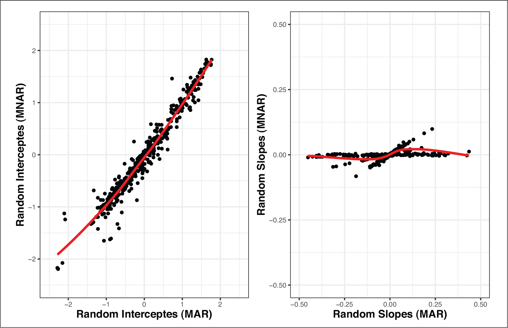
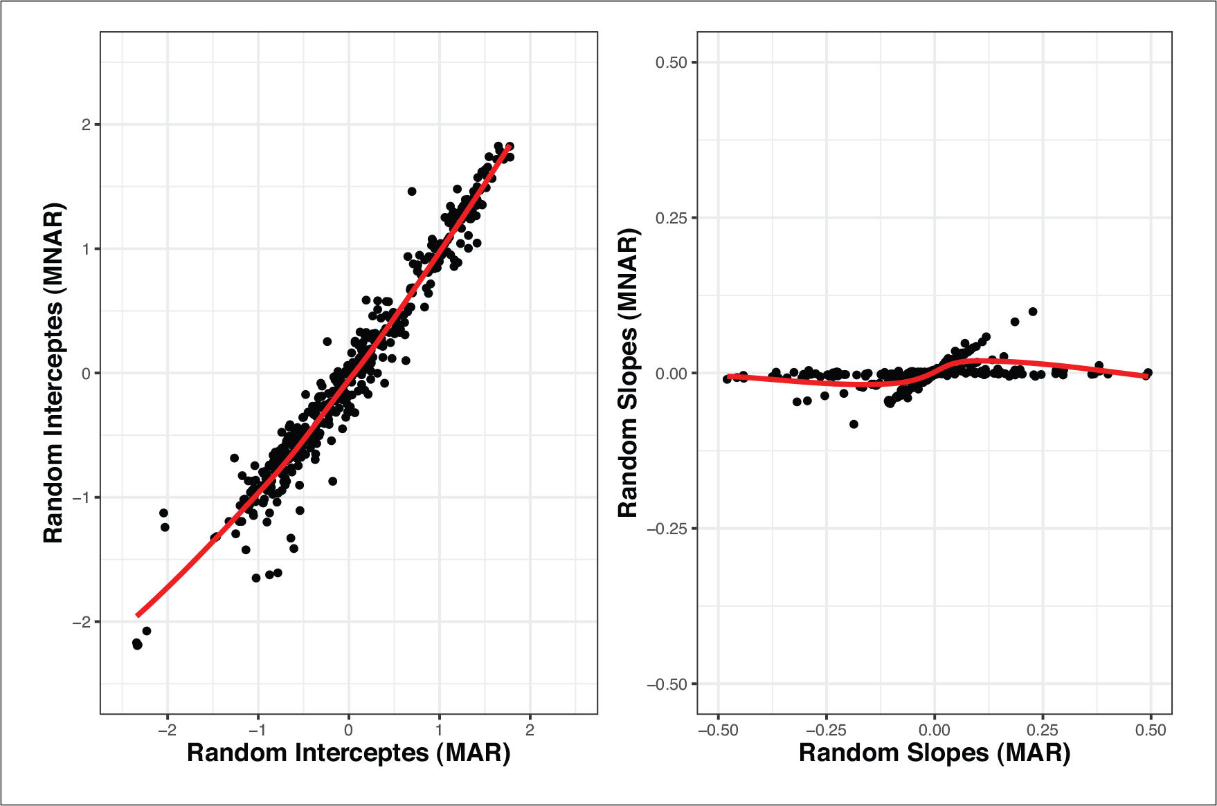
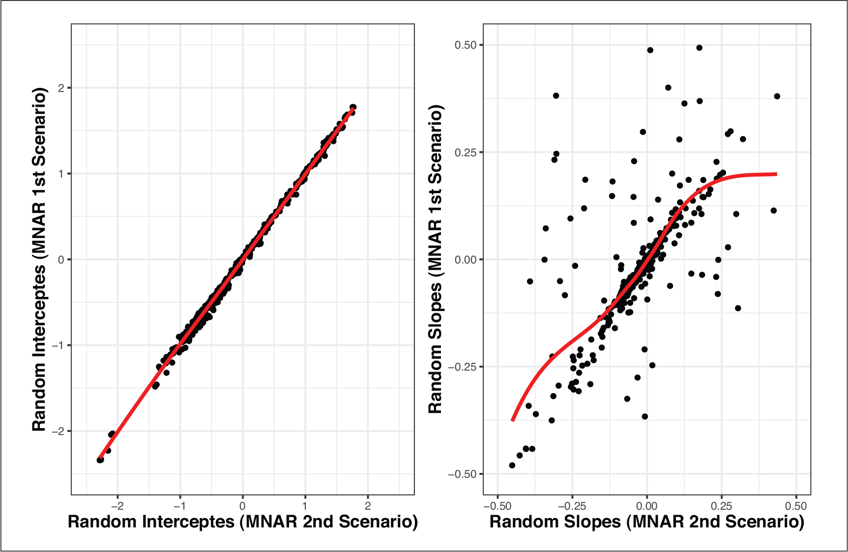
While the results of all the models are close, there are quantitative differences which indicate that the findings might not be stable. This is especially the case when comparing the MAR model with both MNAR models. In Figures 2 and 4, the posterior means of the random effects estimated from the MAR model against the respective estimated random effects from each MNAR model are shown. Similarly, in Figure 5, the posterior means of the random effects estimated from the MNAR model under the 1st Scenario are plotted against the respective estimated random effects from the MNAR model under the 2nd Scenario. These plots give insight into the differences between the three models. We see that especially for the slope components, the differences in the random effects’ estimates are more intense between the MAR model and the MNAR models under both scenarios. These differences become weaker when we compare the MNAR model under the 1st Scenario and the MANR model under the 2nd Scenario, which utilizes the information and distinguishes between dropout due to an event and dropout due to any other reason. This highlights the importance of sensitivity analysis in this context since the differences in the random effects estimates would translate to differences in the subject-specific predictions based on each of the models. The results are stable under different MNAR scenarios, but substantial differences are observed when using an MAR model.
Scenario 1: Posterior means of the random effects under MNAR and MAR
Scenario 2: Posterior means of the random effects under MNAR and MAR
Scenario 2: Posterior means of the random effects under MNAR (1st Scenario) and MNAR (2nd Scenario)
We conducted a simulation study to evaluate the performance of the following three models (used in the analysis of the HIV CD4 data):
Model 1: all dropout cases considered MNAR (as the MNAR model used under Scenario 1 MNAR in the analysis of the HIV dataset), Model 2: all dropout cases considered MAR, Model 3: dropout cases considered MNAR if dropout due to the event or MAR otherwise (as the MNAR model used under Scenario 1 MNAR in the analysis of the HIV dataset),
under different scenarios for the amount of MAR and MNAR dropouts. More specifically, assuming a total dropout rate of 50%, we considered three different scenarios concerning the amount of dropout type: (a) 5% MAR dropouts versus 45% MNAR dropouts, (b) 25% MAR dropouts versus 25% MNAR dropouts and (c) 45% MAR dropouts versus 5% MNAR dropouts. Our goal is to investigate the behaviour between these models under each scenario.
We assumed 600 subjects and then randomly selected follow-up visits,
For the continuous longitudinal outcome, the data were simulated from a linear mixed-effects model as follows:

where 
The values of the parameters were based on the analysis of the HIV CD4 data. For time-to-dropout, we assumed a relative risk model of the form:

where the baseline hazard was simulated from a Weibull distribution
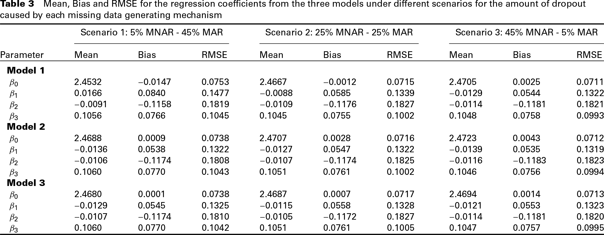
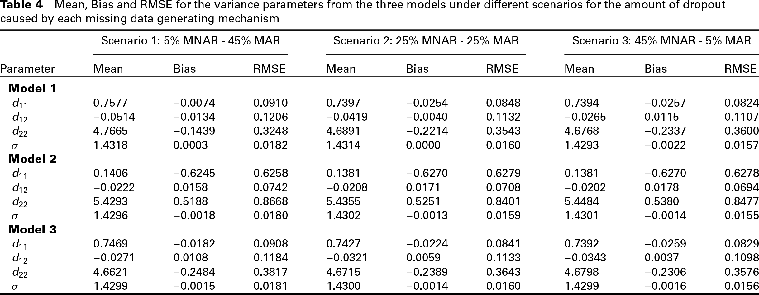
We simulated 500 datasets per scenario, and we fitted each of the three models on each dataset. To assess the behaviour of the three models, we calculated the Bias and Root Mean Squared Error (RMSE) for both the regression coefficients, and the variance parameter estimates. Table 3 summarizes the results for the regression coefficients, while Table 4 summarizes the results for the variance parameters. The results suggest that when the major cause of missingness is MAR, Models 2 and 3 perform similarly and slightly better than Model 1, as far as the regression coefficients are concerned. As the amount of MNAR dropout increases, the three models seem to have similar performance in the estimation of the regression coefficients with only slight differences.
On the other hand, when looking at the Bias and RMSE for the estimates of variance parameters for the random effects, there are more distinct differences between the models. More specifically, the results suggest that Models 1 and 3 perform better than Model 2. Moreover, for the variances of the random effects, under Model 2, the Bias seems to increase as the balance between dropout types moves from MAR dominance to MNAR dominance, whereas the case is the opposite for Model 3. The differences in the variance parameters’ estimates of the random effects between the models also imply that there are considerable differences in the estimated random effects. The difference in the random effects means that the subject-specific predictions derived from these models will differ.
In this article, we have proposed an alternative characterization of MAR for the conventional SPM and proposed its application as a sensitivity analysis tool towards MNAR deviations from the MAR assumption. In doing so, we did not broaden the definition of the SPM by adding additional random effects structures and hence retaining the computational feasibility of the model.
Furthermore, we argued how the subject-specific nature of the MAR characterization in SPM comes with the advantage of more flexible comparisons regarding the causes of missingness. This is an important advantage over other MNAR frameworks such as the PMM and SeM since it allows distinguishing groups of subjects as MAR or MNAR depending on the information available for the causes of missingness. This was illustrated in the application to the HIV data, where we were able to consider different MNAR scenarios with respect to the information available on the causes of missingness.
Mean, Bias and RMSE for the regression coefficients from the three models under different scenarios for the amount of dropout caused by each missing data generating mechanism
Mean, Bias and RMSE for the variance parameters from the three models under different scenarios for the amount of dropout caused by each missing data generating mechanism
Footnotes
Declaration of conflicting interests
The authors declared no potential conflicts of interest with respect to the research, authorship and/or publication of this article.
Funding
The authors would like to acknowledge support by the Netherlands Organization for Scientific Research VIDI (grant number: 016.146.301).