
Abstract
Abstract
Until recently obtaining data on populations of networks was typically rare. However, with the advancement of automatic monitoring devices and the growing social and scientific interest in networks, such data has become more widely available. From sociological experiments involving cognitive social structures to fMRI scans revealing large-scale brain networks of groups of patients, there is a growing awareness that we urgently need tools to analyse populations of networks and particularly to model the variation between networks due to covariates. We propose a model-based clustering method based on mixtures of generalized linear (mixed) models that can be employed to describe the joint distribution of a populations of networks in a parsimonious manner and to identify subpopulations of networks that share certain topological properties of interest (degree distribution, community structure, effect of covariates on the presence of an edge, etc.). Maximum likelihood estimation for the proposed model can be efficiently carried out with an implementation of the EM algorithm. We assess the performance of this method on simulated data and conclude with an example application on advice networks in a small business.
Keywords
Introduction
The last decades have witnessed growing interest in the analysis of relational data. Typically, these data come in the form of a network that displays relations between individuals or objects, and they are represented by means of a graph wherein nodes (i.e., individuals or objects) are connected by edges (i.e., relations). In some applications, especially in genetics, relations cannot be observed directly and the main task is to infer them or their strength from the data (Friedman et al., 2008; Abegaz and Wit, 2013; Vujačić et al., 2015). In this article, we are interested in cases where relations between individuals or objects are observed and the networks themselves are the data.
For a long time, network science was almost exclusively concerned with the analysis of a single network, mainly because of the difficulty in collecting relational data and of limited computing capacity. Statistical modelling of a single network (Snijders, 2011) has typically focused on certain aspects of network topology, such as degree distribution, network statistics or the presence of community structures. This has resulted into the development of a range of statistical network models that include the
More recently, increased computing capacities, alongside with technological advances such as the development of sensor-based measurements, the diffusion of functional magnetic resonance imaging, the invention of high-throughput technologies in biology and the advent of social media, have multiplied the availability of relational data, spurring the analysis not only of larger networks, but also of several instances of the “same” network. The latter includes multilayer networks, dynamic networks and populations of networks. The availability of such collections of several networks poses new modelling challenges. Clearly, when data on several networks are available, modelling each network separately would be inefficient: irrespective of whether we are dealing with multilayer networks, longitudinal networks, or populations of networks, we expect networks therein to be similar to a certain degree; if this is indeed the case, analysing each network separately would not only be cumbersome, but also failing to use the statistical power of the ensemble. Instead, the specification of a joint model for the collection of networks makes it possible to achieve a more parsimonious representation of the data and to borrow information across networks in the estimation process; moreover, such a model may also be employed to identify groups of similar networks. Below, we briefly review some of the solutions that to date have been proposed to tackle this problem in the presence of dynamic networks, multilayer networks or populations of networks.
Dynamic networks allow to represent the evolution of a network system over time. Snijders (2001) proposed a stochastic actor-oriented model where the decision to create or dissolve an edge is based on some covariates, as well as on the current state of the network itself. Hanneke et al. (2010) introduced a dynamic extension of ERGMs, known as temporal ERGM (TERGM). An extension of the latent space models for dynamic networks has been proposed by Sewell and Chen (2015). Matias and Miele (2017), instead, developed a dynamic stochastic blockmodel that allows group membership of units to vary over time.
Multilayer networks are collections of networks that represent different types of relationships (multiple layers) between a group of subjects. Two statistical models that allow to model jointly the layers of those networks are, among others, those of Stanley et al. (2016) and Paul et al. (2016). Stanley et al. (2016) proposed a multilayer stochastic blockmodel that assumes the existence of groups of networks, called strata, that share the same community structure. Paul et al. (2016), instead, introduced a multilayer stochastic blockmodel that assumes that the communities are the same in all layers but allows different block-interaction probabilities in each layer.
Finally, a population of networks can be defined as a collection of independent graphs, each of which corresponds to a different statistical unit. Populations of networks arise, from example, when different individuals are asked to provide their view of relationships within a social network (Krackhardt, 1987) or when brain networks are compared across groups of patients (Taya et al., 2016). Recently, there has been a growing interest in statistical modelling of populations of networks. Sweet et al. (2014) proposed a hierarchical stochastic blockmodel that aims to infer clusters of nodes that are shared across networks. Similarly, Reyes and Rodriguez (2016) introduced a stochastic blockmodel for populations of networks that attempts to identify a unique community structure which is shared across networks. Durante et al. (2017), instead, extended the latent space model approach of Hoff et al. (2002) to populations of networks by proposing a mixture model that describes the joint density of networks in the population using few components, each of which has a different latent-space representation. Finally, Mukherjee et al. (2017) proposed to cluster graphs within a population of networks through a spectral clustering algorithm that is applied to a distance matrix that measures the distances between the graphon estimates of the graphs.
In this article, we focus on the problem of finding and characterizing clusters of graphs that are similar with respect to the effect of certain covariates of interest on the presence or absence of edges in a population of networks. Towards this aim, we propose to model the population of networks with a mixture model whose components can be any statistical network model that can be specified as a generalized linear model (GLM) or a generalized linear mixed model (GLMM); this includes, for example, the
Model specification
We consider a sample of
In principle, one could imagine that each graph
In the presence of many networks, however, this would result in a cumbersome modelling exercise, yielding
Specification of the mixture model
In this article, we consider the existence of clusters of graphs with similar
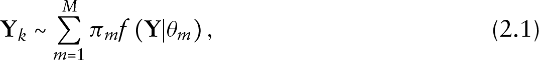
with mixing proportions
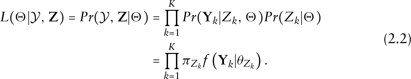
This likelihood suffers from the usual identifiability issues when considering mixture models. Each of the
The way in which the probability density functions
In this article, we focus our attention on network models that assume edges to be independent conditionally on the model parameters (and, potentially, on a set of unobserved random effects), so that their likelihood can be specified as that of a generalized linear (mixed) model. The motivation behind this choice is threefold. Firstly, a wide range of popular network models (among which are the
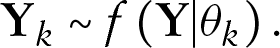
Therefore, we shall specify the mixture model in (2.1) as a mixture of GLMs (Grün and Leisch, 2008) by assuming that the value of each edge
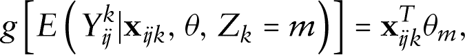
where
model
In social network analysis, the popularity of individuals is often regarded as one of the possible determinants of the formation of relations in a network. This reflects the idea that in certain social settings, individuals may be more likely to relate to popular individuals than to isolated ones: for example, if you live in a small village in the heart of the Alps, you are more likely to interact with popular figures such as the mayor and the priest, rather than with a woodsman who lives in a remote cottage in the middle of the woods. This idea is at the basis of the
Stochastic blockmodel
Besides popularity, group membership of nodes is another factor that can shape the way in which relations are formed. Real networks often feature the presence of communities of nodes whose members are highly connected with each other and tend to form sporadic connections with members from other communities. For example, it has been shown that parliamentarians tend to collaborate more frequently with members from their own parliamentary group rather than with those from other political groups (Signorelli and Wit, 2018). In general, group membership typically induces a so-called community structure in networks, wherein nodes from the same community are closely tied to each other and sporadically linked to nodes from other communities. The effect of community membership on the formation of relations is usually modelled with stochastic blockmodels (Holland et al., 1983; Snijders and Nowicki, 1997). Let

Depending on whether the community-assignment function is known or not, it is possible to distinguish stochastic blockmodels a priori (Holland et al., 1983), wherein community labels are known and interest lies in the reconstruction of relationships between communities, from stochastic blockmodels a posteriori (Snijders and Nowicki, 1997). In this work, we focus on the simpler a priori stochastic blockmodel, which is computationally cheap and, thus, can be easily incorporated into the iterative estimation procedure proposed in Section 3.1. Mixtures of stochastic blockmodels a posteriori, instead, are considered in the works of Stanley et al. (2016) and Reyes and Rodriguez (2016).
The
Clearly, more realistic network models may require a larger set of parameters and this could increase the complexity of maximum likelihood estimation for model (2.1) and computing time. To illustrate this, we consider the extreme scenario of a mixture of saturated network models, where the number of parameters is equal to the number of edge pairs multiplied by the number of subpopulations of graphs, namely
Model estimation
We propose to estimate the unknown parameter vector
EM algorithm
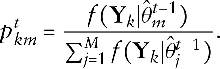
The EM algorithm (Dempster et al., 1977) represents a popular choice for the estimation of mixture models. The algorithm allows the maximization of a likelihood Choose a starting point for the algorithm made by the initial probabilities Given For
In principle, it is possible to initialize the EM algorithm introduced above with any matrix of initial probabilities
Selection of the number of components
In practice, the number of subpopulations
Simulations
In this section, we first evaluate the accuracy of the proposed clustering method with respect to network size (represented by the number of nodes
Clustering accuracy
We begin the assessment of the performance of the proposed method with nine simulations (A-I) where we study the clustering accuracy of our method with respect to the three network models introduced in Section 2.2 as
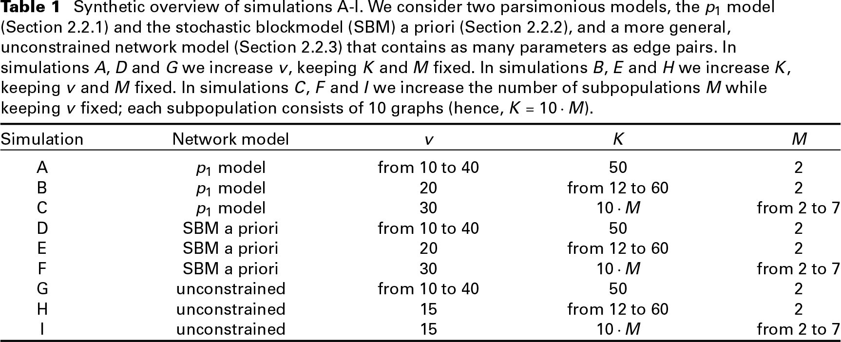
Table 1 summarizes the features of the mixtures of networks considered in each simulation. Within each simulation, we compute 50 repetitions for each combination of
Synthetic overview of simulations A-I. We consider two parsimonious models, the
model (Section 2.2.1) and the stochastic blockmodel (SBM) a priori (Section 2.2.2), and a more general, unconstrained network model (Section 2.2.3) that contains as many parameters as edge pairs. In simulations
,
and
we increase
, keeping
and
fixed. In simulations
,
and
we increase
, keeping
and
fixed. In simulations
,
and
we increase the number of subpopulations
while keeping
fixed; each subpopulation consists of 10 graphs (hence,
).
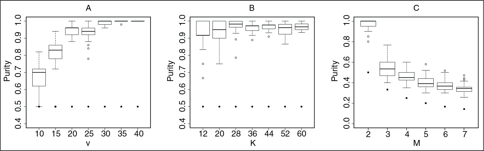
The distribution of purity across repetitions for the
Purity in simulations A, B, C. Each boxplot represents the distribution of purity over 50 repetitions, whereas the squares denote the value of purity that corresponds to a random assignment of graphs to clusters (i.e.,
).
Similar observations hold for the simulations (D, E and F) with the stochastic blockmodel a priori (Supplementary Figure 1) and for those (G, H and I) with the unconstrained network model (Supplementary Figure 2).
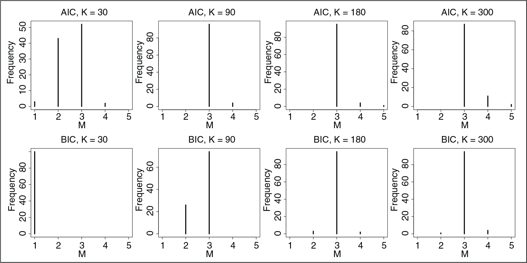
In order to assess the performance of the model selection criteria introduced in Section 3.2, in simulation J we repeatedly sample
Figure 2 shows the distribution of the optimal number of subpopulations obtained with AIC and BIC for the different values of
Distribution of the optimal number of subpopulations in simulation J according to AIC and BIC, for different values of
. The true number of populations is equal to 3.
Distribution of the optimal number of subpopulations in simulation J according to AIC and BIC, for different values of
. The true number of populations is equal to 3.
In Section 4.1, we have considered simulation scenarios with a relatively small number of graphs of moderate size. This has allowed us to show how the proposed approach can achieve a good accuracy in allocating graphs to their correct subpopulation already in problems where
In simulation K, we simulate data from a mixture of stochastic blockmodels a priori with five blocks, setting
Relationship between number of graphs and median computing time in simulation K. It can be observed that computing time is approximately linear in the number of graphs. Computations were performed using a processor with 2.3 GHz CPU.
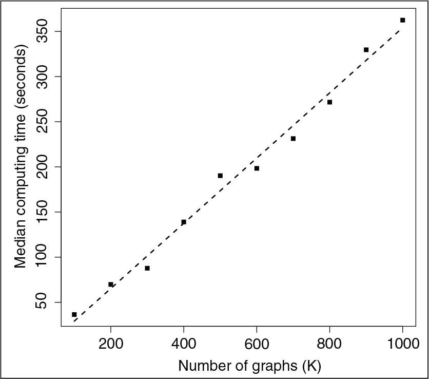
Relationship between number of graphs and median computing time in simulation K. It can be observed that computing time is approximately linear in the number of graphs. Computations were performed using a processor with 2.3 GHz CPU.
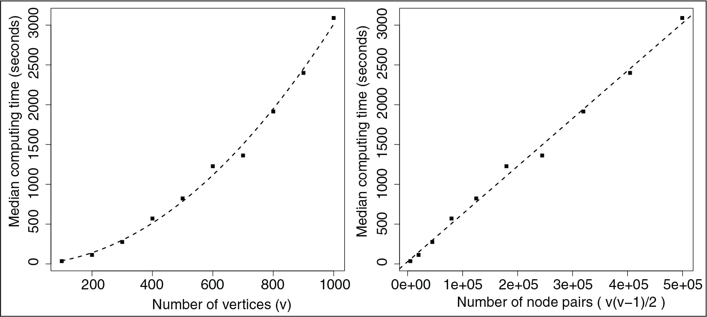
In simulation L, we simulate data from a mixture of stochastic blockmodels a priori with five blocks, setting
Relationship between graph size and median computing time in simulation L. It can be observed that computing time is approximately quadratic in the number of vertices
, and linear in the number of edge pairs
. Computations were performed using a processor with 2.3 GHz CPU.
In this section, we illustrate an application of our model-based network clustering method to a population of networks on advice relationships within a small business collected by Krackhardt (1987), whose aim was to find ways to summarize the reconstructions of an unobserved social network reported by different perceivers. In this study,
Because each employee attempted to reconstruct the actual network of advice relationships within the firm, which is unobserved, we may expect that not only different perceivers would reconstruct advice relationships in a different manner but also some perceivers may provide substantially similar reconstructions of the advice network. In other words, it seems reasonable to hypothesize the presence of different clusters of networks, corresponding to groups of employees who have similar perceptions of advice relationships within the firm.
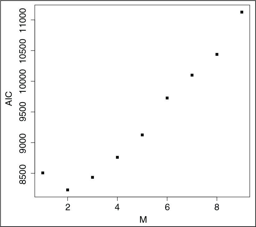
We begin our analysis in an exploratory manner by considering at first a mixture of
The first model that we consider simply assumes that
Value of the AIC for mixtures of unconstrained network models with increasing number of subpopulations
. The minimum AIC is attained when
.
Value of the AIC for mixtures of unconstrained network models with increasing number of subpopulations
. The minimum AIC is attained when
.
Predicted probabilities to observe an arrow from individual
(
-axis) to individual
(
-axis) in the two subpopulations. On both axes, nodes are ordered by department, and horizontal and vertical lines separate employees into the four departments the firm is divided into (so, e.g., employees 6, 8, 12, 17 and 21 belong to department 1; note that employee 7, the CEO, doesn't belong to any department). It is apparent that graphs within the first subpopulation are denser, and that in both subpopulations department affiliation induces a community structure wherein advice relationships are typically more frequent within the same department than between different departments.
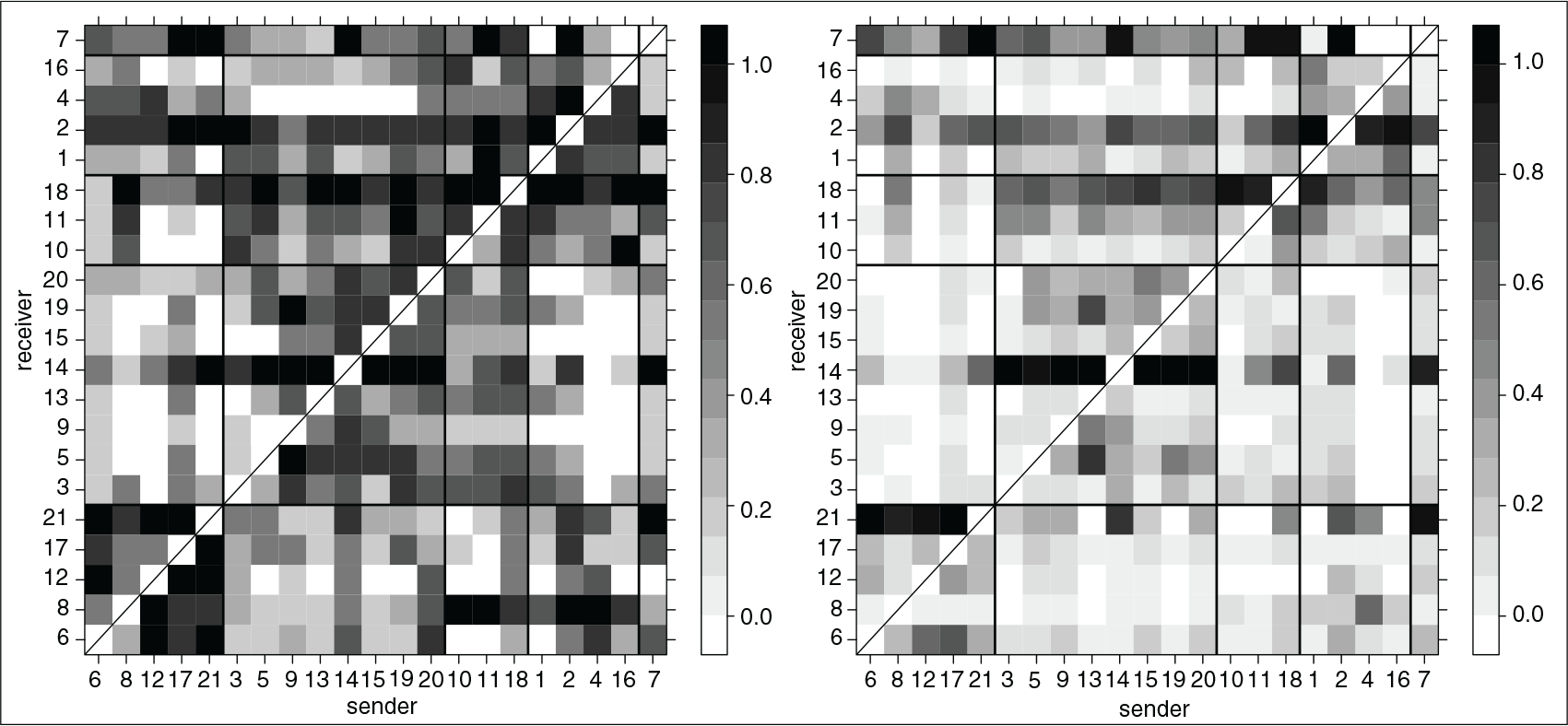
Graphical inspection of Figure 6 clearly reveals that graphs in the first subpopulation are denser than graphs in the second subpopulation; moreover, in both subpopulations we can intuitively observe that department affiliation seems to have a strong influence on the predicted probabilities of advice relationships. However, the large number of parameters (840) employed by the mixture of unconstrained models makes it difficult to draw any further conclusion on similarities and differences between the two subpopulations, and to relate those to any other known feature of the employees. Therefore, we now consider a more parsimonious model where we try to relate the presence of an arrow to such features. Krackhardt (1987) collected the following additional information about the employees:
age and length of service (tenure) of each employee; position occupied by each employee in the firm; one employee is the CEO, two are vice-presidents and the remaining 18 have supervision roles; here, we consider a binary distinction between CEO and vice-presidents on the one hand, and the other 18 employees on the other; the department that each employee belonged to; in total, the firm comprises four departments.
We incorporate these covariates into the analysis by considering a network model where we combine features of the 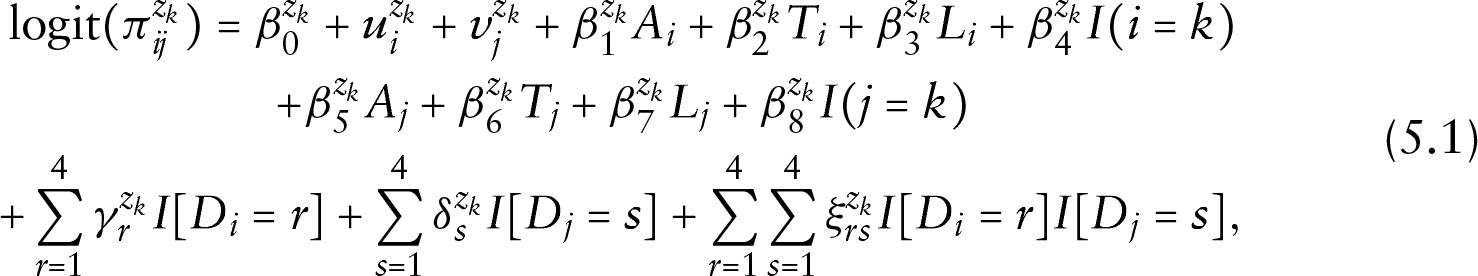
We remark that not only model (5.1) is considerably thriftier than the unconstrained mixture model previously considered (the former comprises 54 parameters, the latter 840), but it is also more interpretable as it enables us to study how the advice relationships reconstructed by the employees could have been affected by individual (age and tenure) and organizational (department and leading roles) features of the employees and firm.
MLEs and standard errors for
in model (5.1), and MLEs of
and
. Asterisks (
) denote regression coefficients that are significantly different from 0 (
) at
level. The last column contains the p-value of the test for equality of each parameter in the two subpopulations (
)
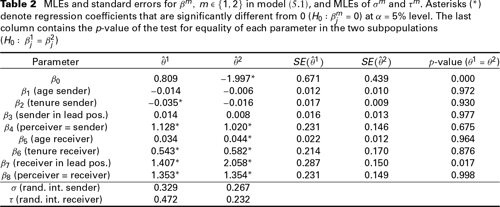
Table 2 contains the MLEs of the fixed effects
Predicted random intercepts for sender (
) and receiver (
) in subpopulations 1 (
-axis) and 2 (
-axis)
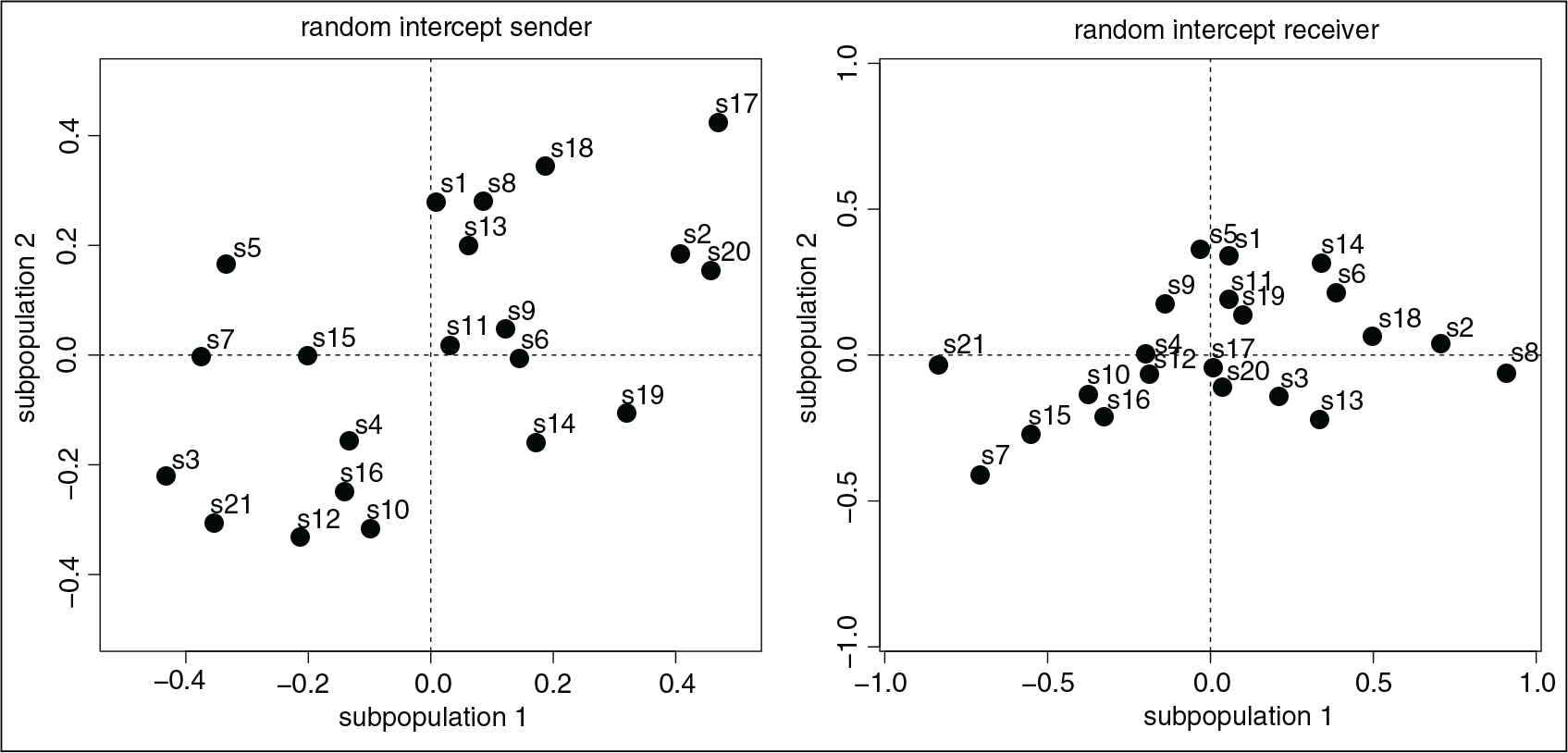
Figure 7 shows the distribution of the predicted random effects for sender and receiver in model (5.1). In the left-hand-side plot, which displays the sender effect, most points fall in the first and third quadrant; this is an indication that perceivers in the two subpopulations have similar ideas on how many colleagues a certain individual seeks advice from. For example, individual 17 has the highest in-degree correction
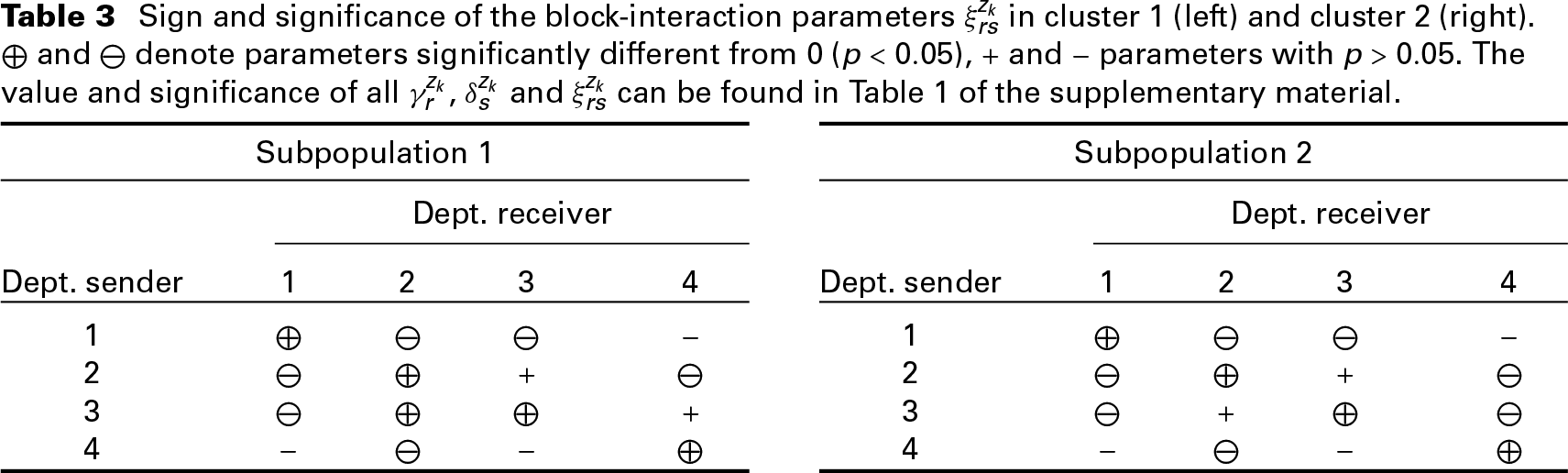
Sign and significance of the block-interaction parameters
in cluster 1 (left) and cluster 2 (right).
and denote parameters significantly different from 0 (
), + and - parameters with
. The value and significance of all
,
and
can be found in Table 1 of the supplementary material.
We have developed a model-based clustering approach for populations of networks that specifies a joint statistical model for all graphs in the population and that is capable of identifying subpopulations of graphs which share a similar generative model, but which may still look like quite different networks in edge-space. Building on the fact that GLMs and GLMMs represent a flexible and efficient tool for modelling and estimating a wide variety of generative processes, we have proposed to employ mixtures of GLMs or GLMMs to perform model-based clustering of networks. Estimation of the proposed mixtures of network models can be efficiently carried out by an EM algorithm. The identification of the number of subpopulations that form the mixture has been performed with standard model selection criteria.
Evaluation of the proposed method on simulated data shows that the accuracy of the clustering method strongly depends on the size of the graphs and on the number of clusters, and much less on the number of graphs in the population. In particular, the accuracy increases quickly with the number of vertices and it decreases, as expected, with the number of clusters. The estimation of the number of subpopulations
The approach presented in this article is able to consider mixtures of network models that make conditional independence assumptions on the probability of existence of edges. Examples of such models include the
Supplementary material
Supplementary material for this article is available online at the link:
Supplemental material for Model-based clustering for populations of networks
Supplemental Material for Model-based clustering for populations of networks by Mirko Signorelli and Ernst C. Wit in Statistical Modelling
Footnotes
Acknowledgements
We thank two anonymous reviewers, whose useful suggestions and remarks have contributed to improve this article.
Declaration of Conflicting Interests
The authors declared no potential conflicts of interest with respect to the research, authorship and/or publication of this article.
Funding
The authors gratefully acknowledge funding from the COST Action European Cooperation for Statistics of Network Data Science (CA15109).