
Abstract
Abstract:
In social and economic studies many of the collected variables are measured on a nominal scale, often with a large number of categories. The definition of categories can be ambiguous and different classification schemes using either a finer or a coarser grid are possible. Categorization has an impact when such a variable is included as covariate in a regression model: a too fine grid will result in imprecise estimates of the corresponding effects, whereas with a too coarse grid important effects will be missed, resulting in biased effect estimates and poor predictive performance.
To achieve an automatic grouping of the levels of a categorical covariate with essentially the same effect, we adopt a Bayesian approach and specify the prior on the level effects as a location mixture of spiky Normal components. Model-based clustering of the effects during MCMC sampling allows to simultaneously detect categories which have essentially the same effect size and identify variables with no effect at all. Fusion of level effects is induced by a prior on the mixture weights which encourages empty components. The properties of this approach are investigated in simulation studies. Finally, the method is applied to analyse effects of high-dimensional categorical predictors on income in Austria.
Introduction
Researchers in medicine, social and economic sciences routinely collect data measured on a nominal scale as potential predictors in regression models. The usual approach to include such categorical predictors in regression type models is to define one category as the baseline or reference category and use dummy variables for the effects of all other categories with respect to this baseline. Thus, the effect of one categorical covariate with
In order to avoid the risk of overlooking substantial differences in level effects, it would be appealing to have a method which allows to start with a large regression model including categories on a very fine classification grid and to obtain a sparser representation of this model during estimation. Sparsity can be achieved whenever the effects of a categorical predictor can be represented by less than
Usually, sparsity in regression type models is achieved by applying variable selection methods which allow to identify regressors with non-zero effects, that is, lasso (Tibshirani, 1996) or the elastic net (Zou and Hastie, 2005) in the frequentist framework and shrinkage priors (Park and Casella, 2008; Griffin and Brown, 2010) or spike and slab priors (Mitchell and Beauchamp, 1988; George and McCulloch, 1997; Ishwaran and Rao, 2005) in the Bayesian framework. However, these methods are not appropriate for categorical covariates as only single level effects are selected or excluded from the model. Approaches that address exclusion of a whole group of regression effects have been proposed by Chipman (1996), Yuan and Lin (2006), Raman et al. (2009), Kyung et al.(2010) and recently by Simon et al.(2013), but none of these approaches allows also for effect fusion.
For metric predictors, effect fusion can be performed by the fused lasso (Tibshirani et al., 2005) and the Bayesian fused lasso (Kyung et al., 2010). Both methods assume some ordering of effects and shrink only effect differences of consecutive levels to zero, and hence are not appropriate for nominal predictors where any pair of level effects should be subject to fusion. Explicit effect fusion for nominal predictors is considered in Bondell and Reich, (2009) and by Gertheiss and Tutz (Gertheiss and Tutz, 2009; Gertheiss and Tutz, 2010; Gertheiss et al., 2011; Tutz and Gertheiss, 2016), who specify lasso-type penalties on effects and effect differences. In a Bayesian approach, recently Pauger and Wagner (2017) specified a prior distribution that can be interpreted as a spike and slab prior on effects and effect differences. However, these approaches are limited to covariates with a moderately large number of categories, as for a covariate with
An appealing approach for effect fusion which avoids classification of effect differences and allows to fuse effects directly is to use model-based clustering techniques. Basford and McLachlan (1985) considered clustering of treatment effects in analysis of variance (ANOVA) by specifying a finite mixture of Normal components on the observed treatment means and fit the model via an EM algorithm. In regression models, sparse modelling of effects by mixtures is so far primarily used for continuous covariates. Yengo et al. (2014) and Yengo et al. (2016) define a Normal mixture prior for the regression effects and determine the number of components, that is, coefficient groups, using model choice criteria. In a non-parametric framework, MacLehose and Dunson (2010) use an infinite mixture of heavy-tailed double-exponential distributions on the coefficients of continuous predictors to allow groups of coefficients to be shrunk towards the same, possibly non-zero, mean. Only Dunson et al. (2008) consider categorical covariates. They propose a multi-level Dirichlet process prior on the effects of single nucleotide polymorphism (SNP) in genetic association studies. This prior takes the hierarchical structure of the predictors into account and allows clustering of SNPs both within and across genes. However, by considering 22 markers, each with three levels, only a small number of levels is investigated.
Following this line of research we propose to achieve model-based clustering of level effects by specifying a finite Normal mixture prior. Our approach is explicitly designed to address effect fusion for categorical covariates and has several advantageous features.
First, fusing the level effects directly instead of focusing on all effect differences enables us to handle categorical covariates with a large number of categories, for example, 100 or more. Second, the specified mixture prior can be interpreted as a generalization of the standard spike and slab prior (George and McCulloch, 1993) where a spike distribution at zero is combined with a rather flat slab distribution to allow selective shrinkage of effects; see Malsiner-Walli and Wagner (2011) for an overview. We replace the slab distribution by a location mixture distribution with different, non-zero means. This mixture prior allows to shrink non-zero effects to various non-zero values and introduces a natural clustering of the categories: if level effects are assigned to the same mixture component, they are assumed to be (almost) identical and can be fused.
Third, the hyperparameters of the mixture prior are chosen very carefully to achieve the modelling aims. Their specification is based on the data to yield recommendations that are applicable to a wide range of real data situations. The ‘fineness’ of the estimated level classification can be guided by the size of the specified component variance, with smaller variances inducing a larger number of estimated effect groups. The prior on the mixture weights is specified following the concept of ‘sparse finite mixture’ (Malsiner-Walli et al., 2016). Specifying a sparsity inducing prior on the weights in an overfitting mixture avoids unnecessary splitting of superfluous components and encourages concentration of the posterior distribution on a sparse cluster solution and thus allows to estimate the number of effect groups from the data.
Fourth, remaining in the framework of finite mixture of Normals and conditionally conjugate priors avoids a computationally intensive estimation as standard Markov chain Monte Carlo (MCMC) methods can be used. The MCMC scheme for posterior inference basically combines a regression and a model-based clustering step, where in both only standard Gibbs sampling steps are needed.
Finally, model selection is based on the posterior draws of the partitions. Two strategies are pursued to select the final partition of the levels, by either selecting the most frequently sampled model or determining the optimal partition of the effects based on their joint posterior fusion probabilities.
The article is organized as follows. In Section 2 the model and the prior distributions for the model parameters are introduced. Details on posterior inference and model selection are given in Section 3. The method is evaluated in a simulation study in Section 4 and applied to a regression model for income data in Austria in Section 5. Finally, Section 6 concludes.
Effect clustering prior
We consider a standard linear regression model with observations

To complete Bayesian model specification, prior distributions have to be assigned to all model parameters. We assume that regression effects are independent between covariates and use a prior of the structure

Our goal is to specify a prior for the level effects of covariate
The prior on a regression effect


An alternative to our finite mixture approach would be to specify an infinite mixture where a Dirichlet process prior
Additionally, it has to be pointed out that the clustering behaviour of finite and infinite mixtures is quite different. For infinite mixtures, the a priori expected number of groups when classifying
The specification of the prior hyperparameters is crucial to achieve our modelling aims. To obtain recommendations that are applicable to a wide range of situations, we take an empirical approach and choose the hyperparameters depending on the data.
The location parameter of the first mixture component
Level effects should be assigned to the same component only if the sizes of their effects are almost identical. Therefore, specification of the component variance
We define the component variance
Figure 1 shows the prior distributions of the level effects of one of the covariates in our application, the covariate
Finite mixture prior on level effects of covariate economic sector for two different mixture component variances,
(left panel) and
(right panel). One component is centred at zero (blue dashed line), the others at
,
under flat prior
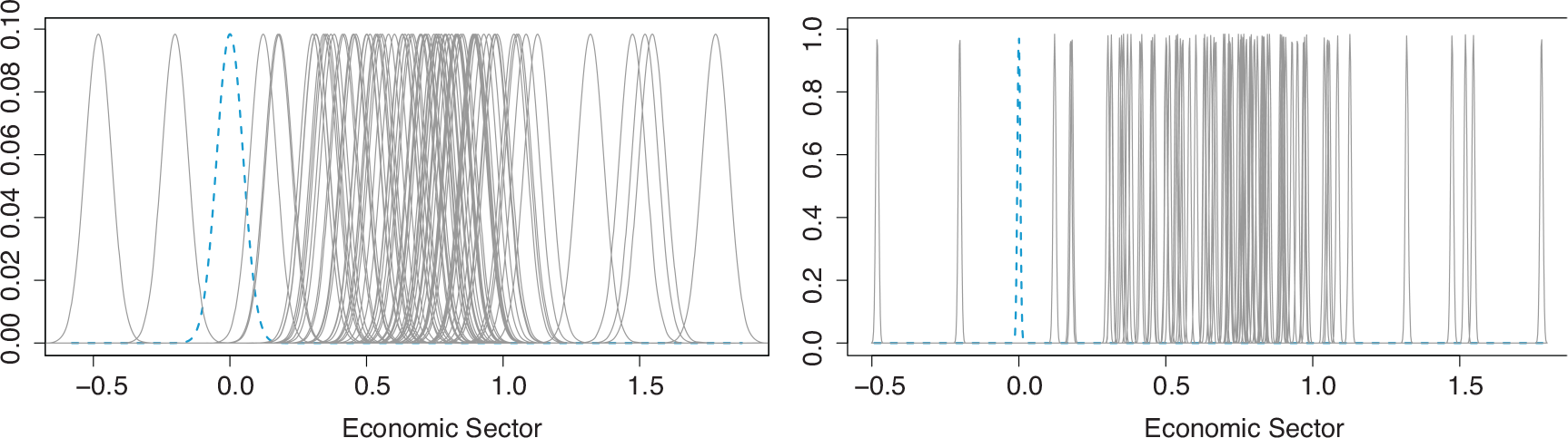
Finite mixture prior on level effects of covariate economic sector for two different mixture component variances,
(left panel) and
(right panel). One component is centred at zero (blue dashed line), the others at
,
under flat prior
Since the choice of the prior component variance
We now turn to the specification of the number of mixture components
Rousseau and Mengersen (2011) investigated the asymptotic behaviour of the posterior distribution of an overfitting mixture model and showed that the hyperparameter
Following Malsiner-Walli et al. (2016); Malsiner-Walli et al. (2017), Nasserinejad et al. (2017) and Frühwirth-Schnatter (2017), we choose
The posterior distribution, which results when combining the likelihood derived from equation (2.1) with the prior distribution of
However, though model averaged estimates of the coefficients may give good results in terms of prediction, researchers are often interested in selection of a final model and interpretation of its results. In regression models with categorical predictors, model selection is more involved than in standard variable selection, as the problem is to determine an appropriate clustering of level effects, which means that both the number of clusters as well as the members of each cluster have to be determined. We address this problem in Section 3.3, where we present two different strategies for model selection when clustering the effects of a categorical covariate.
MCMC sampling
Model estimation is performed through MCMC sampling based on data augmentation (Diebolt and Robert, 1994; Frühwirth-Schnatter, 2006). For each covariate

MCMC sampling is basically performed by iterating two steps: the regression step, where the level effects and the error variance are sampled conditional on knowing the mixture components the effects are assigned to, and the model-based clustering step, where the parameters of the mixture components and the latent allocation variables are sampled. In the starting configuration, each level effect
The MCMC sampling scheme iterates the following steps:
Regression steps
1. Sample the regression coefficients 2. Sample the error variance Model-based clustering steps
3. For 4. For 5. If a hyperprior is specified on 6. Sample the latent allocation indicators

Model-averaged estimates
MCMC draws approximate the whole posterior distribution taking into account model uncertainty: for example, for a regression effect

Model selection
Before performing model selection, generally the samples from the mixture model have to be identified. In the Bayesian framework, identification of a finite mixture model requires handling the ‘label switching’ problem (Redner and Walker, 1984) which is caused by the invariance of representation (2.3) with respect to reordering the components:

After MCMC sampling, there are several options to summarize the posterior clustering distribution and to select a final partition of the level effects of covariate
Another option to select the final partition is to average the matrix
Similar to
An advantage of this approach is that clusters of effects are correctly identified even if distances are high, that is, joint inclusion probabilities are rather small. This can happen if the number of categories is large and the strong overlapping of the mixture components induces a frequent switching of the levels between the components, so that the inclusion probability of any two level effects become small, and the most frequent model is not a good representative of the sampled models. However, a drawback of this approach is that the silhouette coefficient cannot be computed for a one-cluster solution. Therefore, with this strategy it is not possible to identify the case where all level effects are assigned to the zero component and the corresponding predictor can be excluded from the model.
Simulation study
A sparser representation of the effects of a categorical covariate is possible when (a) some or (b) all of the levels have no effect or (c) some levels have the same effect and hence can be fused. To investigate the performance of the proposed prior distribution in these situations, we perform a simulation study where categorical covariates with moderate as well as large number of levels represent the various types of sparsity. We evaluate both model selection strategies proposed in Section 3.3, that is, using either the most frequent sampled partition or the partition selected by performing PAM and the silhouette coefficient, with respect to correct model selection. Further, we determine estimation accuracy and predictive performance of the estimates based on the selected models as well as the model averaged estimates.
Set-up
We define a regression model according to (2.1) with four independent categorical predictors, the first three predictors having 10 and the forth 100 categories. All categories have uniform prior class probabilities. The level effects of the first covariate have three different values (
MCMC sampling is run for 15 000 iterations after a burn-in of 15 000. The final model is chosen by employing both model selection strategies suggested in Section 3.3. The selected models are then refitted under a flat Normal prior
In order to compare the different final models, two model choice criteria, the Deviance Information Criterion (DIC), proposed by Spiegelhalter et al. (2002), and the BICmcmc, suggested by Frühwirth-Schnatter (2011), are performed. Both measures rely on the MCMC output and can be easily computed. BICmcmc is determined from the largest log-likelihood value observed across the MCMC draws. Whereas the classical BIC is independent from the prior, BICmcmc depends also on the prior of the regression parameters.
Model selection results
The model selection results are evaluated by reporting the estimated number of level effect groups. Additionally, the clustering quality is assessed by calculating the adjusted Rand index (Hubert and Arabie, 1985), the error rate, the false negative and the false positive rate.
The adjusted Rand index (AR) allows to quantify the similarity between the true and estimated partition of the level effects (Hubert and Arabie, 1985). It is a corrected form of the Rand index (Rand, 1971), adjusted for chance agreement. A value of
The error rate (err) of the clustering result is the number of misclassified categories divided by all categories. It should be as small as possible. Since interest mainly lies in avoiding incorrect fusion of categories rather than unnecessary splitting of ‘true’ groups, additionally false negative rate (FNR) and false positive rate (FPR) are reported. They are defined as

Table 1 shows the clustering results for all four covariates using both model selection strategies, that is, the most frequent model (‘most’) and the model selected using PAM (‘pam’), for fixed component variance
Model selection results for fixed
with
. Comparison of the two model selection strategies ‘most’ and ‘pam’. The first three variables have 10 categories, the 4th variable 100 categories. FNR is not defined for variable 3
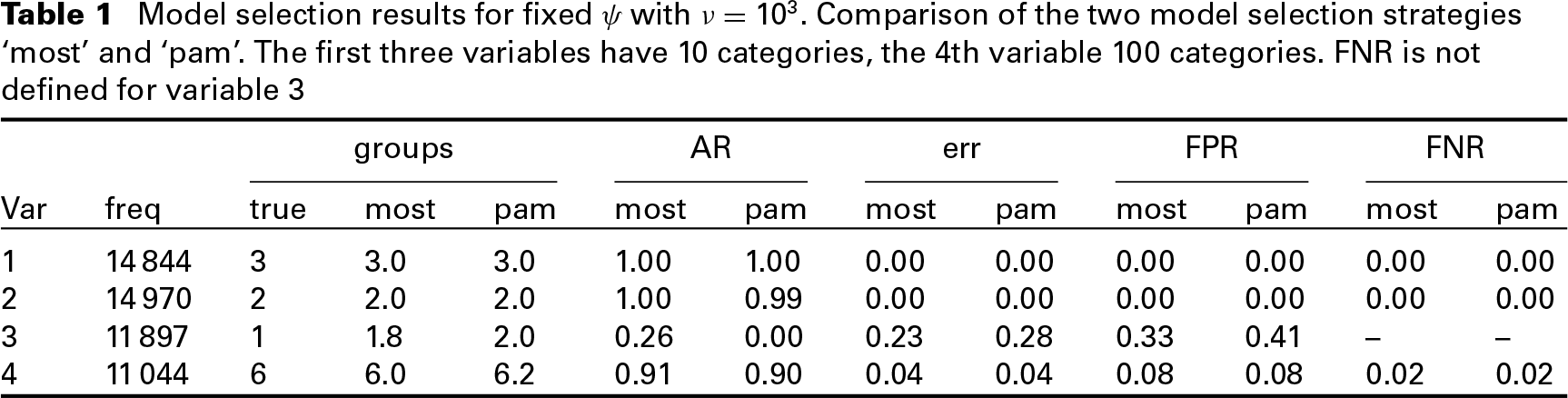
Model selection results for fixed
with
. Comparison of the two model selection strategies ‘most’ and ‘pam’. The first three variables have 10 categories, the 4th variable 100 categories. FNR is not defined for variable 3
In order to compare our clustering results to those obtained following the approach proposed by Gertheiss and Tutz (2010) and Oelker et al. (2014), we use the
Penalty approach: Model selection results
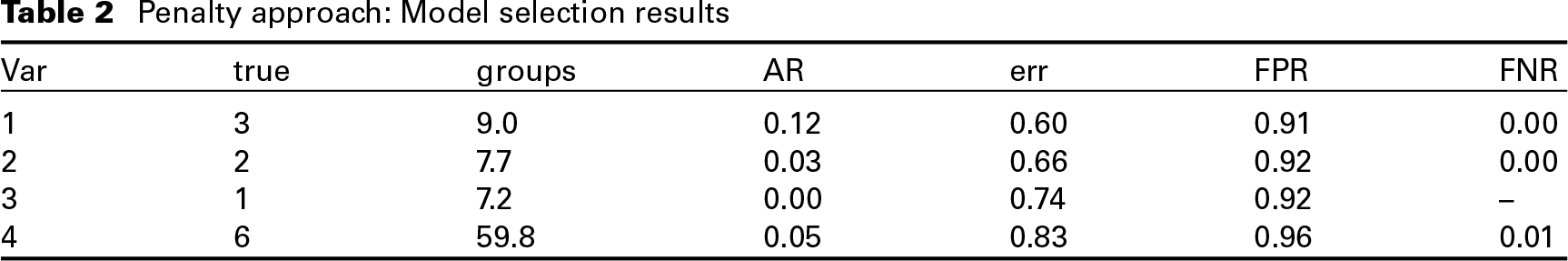
To investigate the impact of the component variances
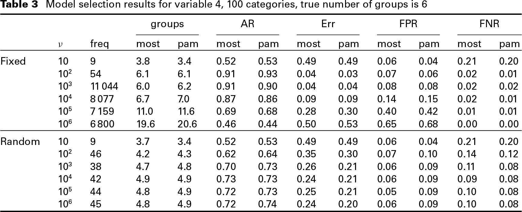
When a hyperprior on the component variances is specified as described in Section 2.1, the true number of effects is captured well for variables 1 to 3, where the true number of clusters is at most three (see Tables C.1–C.3). However, for covariate 4 with six different effects, the true number of effect groups is underestimated, regardless of the employed model selection strategy, see Table 3. Although for larger values of
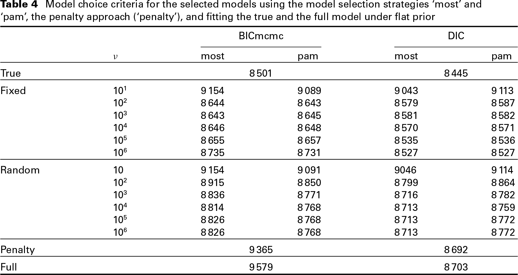
Table 4 shows that all models with fixed or random component variance outperform the full model with respect to the BICmcmc; models with a fixed component variance outperform the full model even in terms of DIC unless the component variance is large (i.e., for
Model selection results for variable 4,
categories, true number of groups is
Model choice criteria for the selected models using the model selection strategies ‘most’ and ‘pam’, the penalty approach (‘penalty’), and fitting the true and the full model under flat prior
Finally, accuracy and predictive performance of the approach is evaluated by computing the mean squared error (MSE) of the coefficient estimates and the mean squared predictive error (MSPE). The results are compared to those of the full model, the true model and using penalized ML-estimates, and are reported in Appendix C.
We illustrate the proposed approach for effect fusion in an application to data from EU-Statistics on Income and Living Conditions (SILC) survey 2010 in Austria. Relying on a questionnaire, the EU-SILC data are the main source for statistics on income distribution and social inclusion at the European level, see Statistics Austria (
As potential regressors, we consider the continuous covariate
The economic
We standardize the response
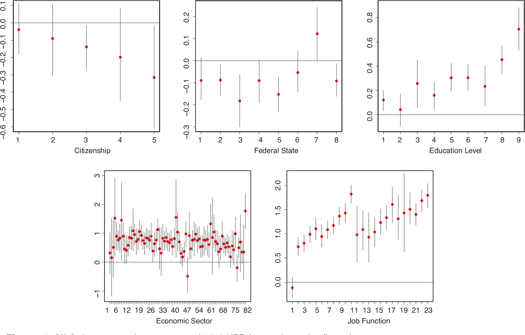
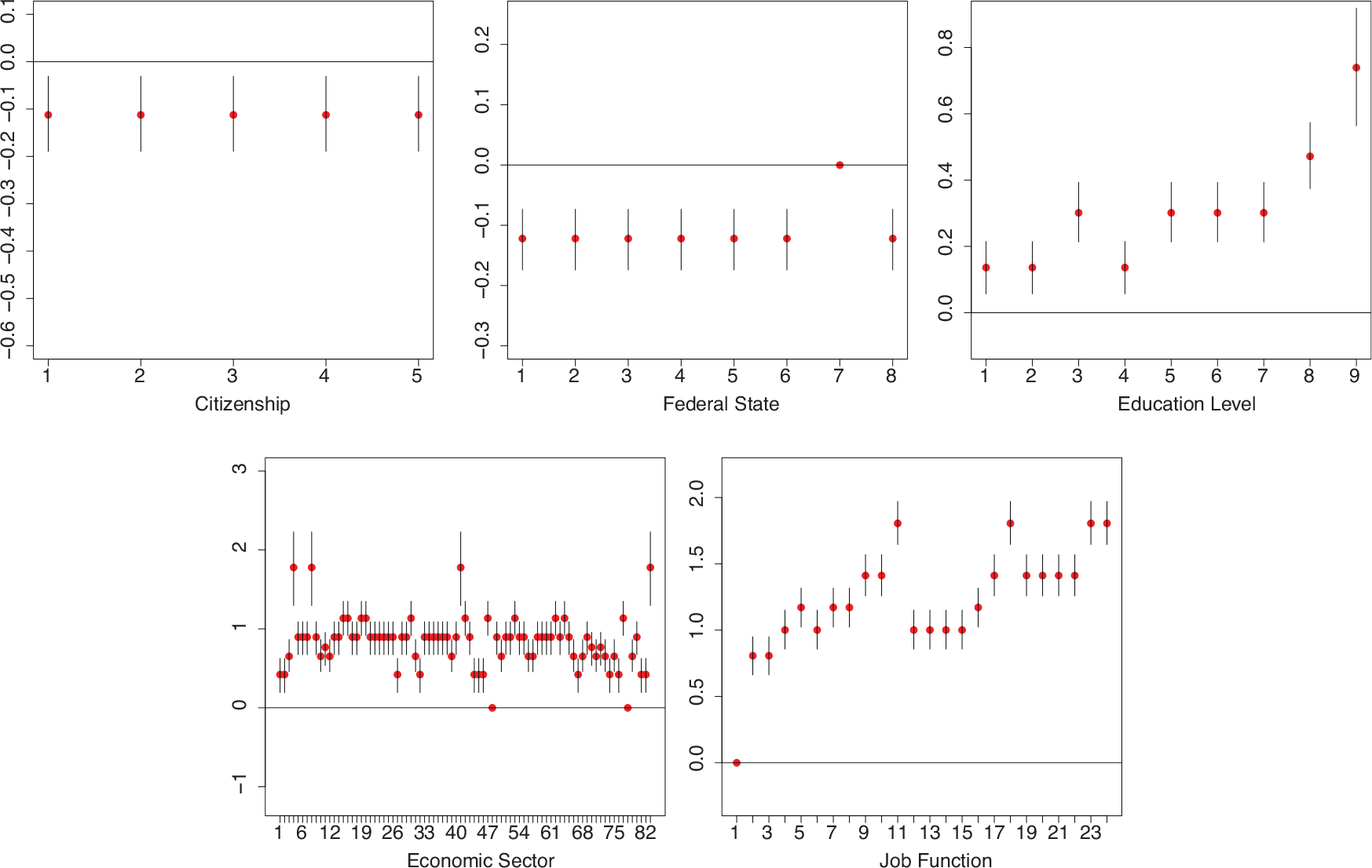
SILC data, posterior means and 95% HPD intervals under flat prior
We fit regression models with prior specifications as described in Section 2, with fixed and random component variances,
SILC data: estimated number of level groups for the categorical covariates and BICmcmc for various scaling factors
, with fixed and random component variances
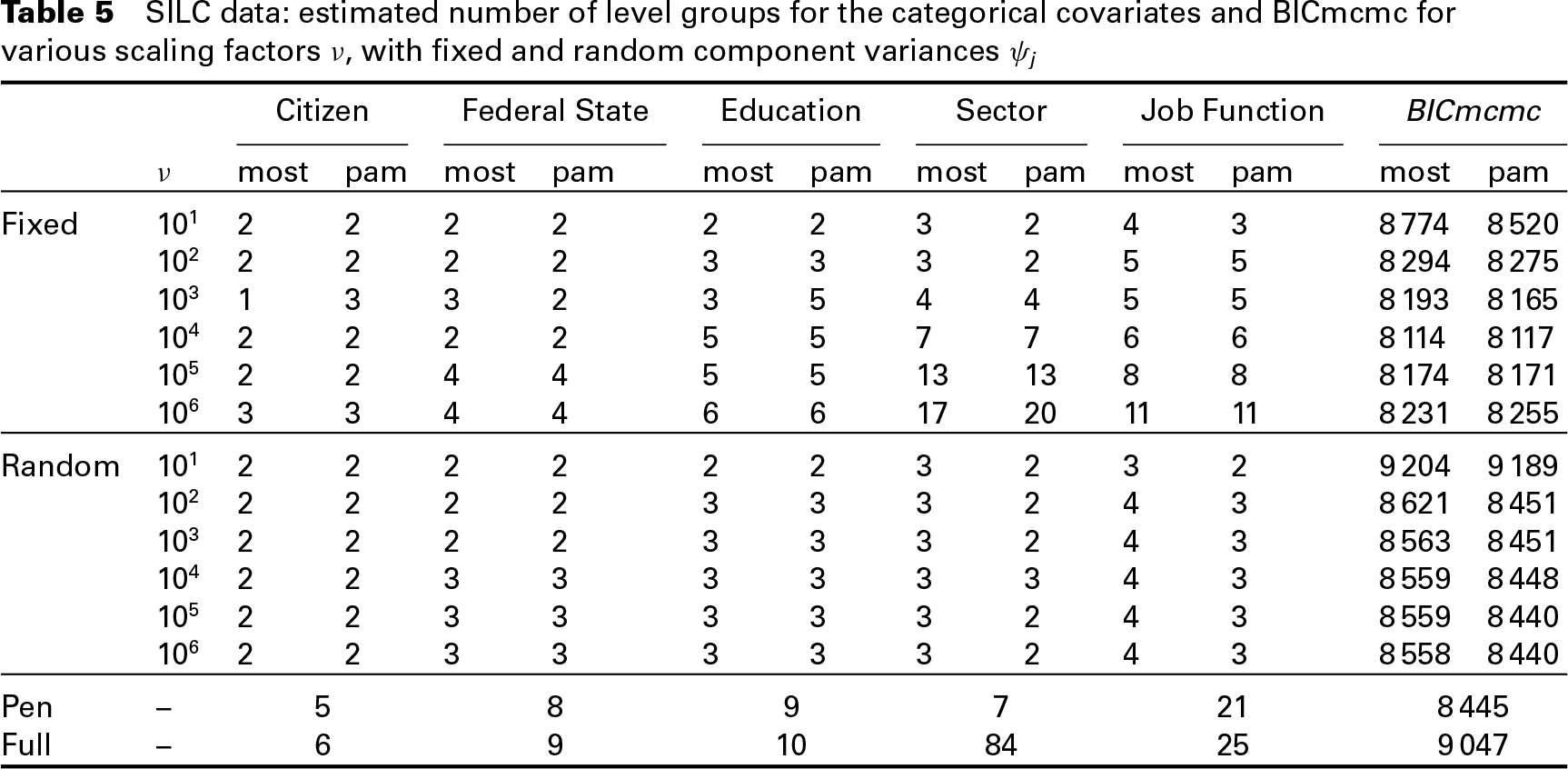
For fixed
SILC data, posterior means and 95% HPD intervals under mixture prior with
and fixed variance specification
To visualize the cluster solutions for different values of
SILC data, variable ‘job function’: Level estimates with 95% HPD intervals for various
(from top left), by selecting the most frequent model and with fixed component variance
. In the last plot on the bottom right, the dotted lines indicate the 5 categories of the first level of aggregation, see Table D. 1
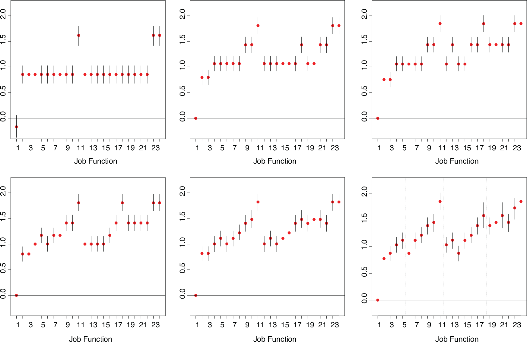
With a hyperprior on the component variance
In this article, we proposed to specify a finite Normal mixture prior on the level effects of a categorical predictor to obtain a sparse representation of these effects. The mixture specification allows to shrink non-zero effects to different non-zero locations and introduces a natural clustering of the level effects. Level effects assigned to the same mixture component are fused, that is, their effects are replaced by the same joint effect. The number of components as well as their locations are treated as unknown and estimated from the data. A sparse prior on the mixture weights helps to avoid unnecessary splitting of non-empty components and to concentrate the posterior distribution on a sparse cluster solution. The number of estimated level groups can be guided by the size of the component variances, with a smaller variance inducing a larger number of estimated effect groups.
We noted that surprisingly the specification of a hyperprior on the component variances did not work well. In contrast to the common clustering of known data points, we aim at clustering of regression effects, which are not fixed but have to be estimated themselves. Assigning an effect to a mixture component corresponds to selecting a particular prior distribution for its estimation, and hence has an impact on its value in the next parameter estimation step. Thus, additional uncertainty is introduced when clustering regression effects. This leads to the estimation of large component variances and only few effect groups, if the component variances are allowed to be random. Therefore, we recommend to fix the variances of the mixture components and investigate the resolution of level effects with different values. To select the final model, model choice criteria can be used. A strength of our approach is that the spike variance specification can vary across the variables, which allows the researcher to obtain a ‘finer’ clustering for effects of particular interest.
We investigated two different model selection strategies. We selected either the model sampled most frequently or applied the PAM clustering algorithm (Kaufman and Rousseeuw, 2005) to the matrix of posterior inclusion probabilities and selected the final model maximizing the silhouette coefficient of the obtained clusterings. Both strategies have shown to perform similar. An advantage of the first strategy is that a one-group solution can also be selected, which is not possible for the ‘PAM’ strategy, but the latter is robust against the switching of single effects between groups.
The approach works well even if the number of categories is high, for example, around 100. For Gaussian response regression models, the computational effort is low as a standard Gibbs sampling scheme can be used for MCMC estimation. The sampling scheme is implemented in the
Acknowledgements
This research was financially supported by the Austrian Science Fund FWF (P25850, V170 and P28740) and the Austrian National Bank (Jubiläumsfond 14663). We want to thank Bettina Grün from the Department of Applied Statistics, Johannes Kepler University Linz, for many fruitful discussions.