Sage Journals: Discover world-class research

Abstract

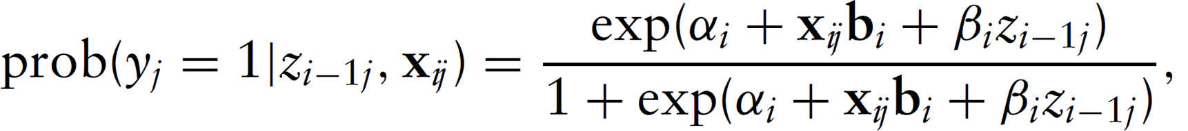
Sequential regression approaches can be used to analyze processes in which covariates are revealed in stages. Such processes occur widely, with examples including medical intervention, sports contests and political campaigns. The naïve sequential approach involves fitting regression models using the covariates revealed by the end of the current stage, but this is only practical if the number of covariates is not too large. An alternative approach is to incorporate the score (linear predictor) from the model developed at the previous stage as a covariate at the current stage. This score takes into account the history of the process prior to the stage under consideration. However, the score is a function of fitted parameter estimates and, therefore, contains measurement error. In this article, we propose a novel technique to account for error in the score. The approach is demonstrated with application to the sprint event in track cycling and is shown to reduce bias in the estimated effect of the score and avoid unrealistically extreme predictions.

Keywords

logistic regression measurement error sequential regression staged processes track cycling

1 Introduction

Consider a stochastic control process or prediction problem in which a random outcome depends on a set of non-random covariates such that (a) disjoint subsets of the covariates are revealed in stages and (b) at each stage, a model (explanatory or predictive) for the outcome is required. Such processes, which have a natural order given by the discretization of time into stages, occur in many fields: for example, medics may wish to model patient survival prior to intervention, immediately post intervention, and prior to discharge taking account of patient, disease and intervention characteristics revealed at each stage; in a sporting context, coaches and players would like to understand the effect of tactical decisions on overall outcome as the contest progresses; and politicians may wish to assess the effectiveness of tactics used during various stages of a political campaign. At each stage, a vector of covariates is revealed, and a modeller/statistician might take one of the following approaches:

At each stage $i = 1, . . ., m$ , fit a model that contains the covariates revealed up to and including stage i, repeating this process at each stage (naïve sequential regression).

At the first stage, fit a model that contains the covariates revealed at the first stage, and then at each stage $i = 2, . . ., m$ , fit a model that contains the covariates revealed at stage i plus the estimated linear predictor from the previous stage $i - 1$ . Elisheva et al., (2000) refer to models, obtained in this way as sequential models and we will follow their convention of referring to the linear predictor as the score throughout this article.

The naïve approach (1) may be practical if both the total number of covariates and the number of stages are not too large. Otherwise, we should anticipate difficulties regarding covariate selection: for example, if a covariate enters the model at stage i, should it enter the model at all stages, or should its selection at stage i not influence selection at other stages? A solution to this problem is to proceed sequentially as in approach (2), so that a covariate that enters the model at stage i continues to have an effect at all subsequent stages, albeit becoming more dilute as the sequential model fitting proceeds. Approaches (1) and (2) are considered further in Section 2.

A drawback of the sequential approach (2) is that the estimates of the covariate effects can be biased since the score is itself a random variable. This article develops a measurement error model to alleviate this problem and, to our knowledge, is the first to do so. In particular, we describe a measurement error model for sequential generalized linear models (GLMs); we do this in Section 3, with a particular focus on sequential logistic regression. We will call our approach sequential measurement error regression. The approach is demonstrated in Section 4 by application to the sprint event in track cycling; here, the object is to explain race outcome at each of a number of intermediate stages in the race. The novel technique we develop avoids biases in the estimates of the effect of the score at each stage and, hence, is essential for making appropriate inferences about the size of covariate effects. In the example we describe, such biases were up to 19%, when measured relatively to the size of the effect. We also demonstrate that the difference in the predicted probabilities of overall outcome, between the standard sequential approach (2) and the sequential measurement error approach, propagates through the stages leading to unrealistically high or low values of the predicted probability when not accounting for measurement error.

2 Review of the statistical analysis of sequential processes

A key feature of such sequential processes is that the number of influential covariates increases with each stage, since the model at stage i should consider all covariates revealed so far in the process. If there are too many influential covariates compared to the number of cases, the variability in the parameter estimates becomes large (Peduzzi et al., 1996; Vittinghoff and McCulloch, 2007). Vittinghoff and McCulloch (2007) suggest that there should be at least five events per covariate (an event being the outcome, either success or failure, whichever occurs least often). Therefore, the naïve approach (1) will not be applicable for many processes. Each stage could be considered in isolation, by fitting a model with only the covariates revealed in the current stage. However, this can lead to the effect of covariates being misinterpreted. In particular, covariates at one stage may act as surrogates for other covariates revealed in earlier stages. For example, Hill et al. (2000), when studying coronary artery bypass treatment, developed a model containing covariates relating to a bypass operation as well as a covariate to capture pre-operative factors. They found that one of the operative covariates did not significantly affect outcome, in contrast to an earlier study that did not account for pre-operative factors.

To overcome this problem, Elisheva et al. (2000), Hill et al. (2000), Van Wermeskerken et al. (2000) and Welsby et al. (2002) used the estimated score (or the implied outcome probability) from the model developed at the previous stage as a covariate in place of all covariates revealed in the prior stages, that is, approach (2) of Section 1. This estimated linear predictor or estimated score (or its equivalent) is effectively a collective covariate describing the influential covariates prior to the current stage. However, the sequential logistic regression approach of Elisheva et al. (2000) makes the assumption that the score is a non-random covariate when it is, in fact, a random variable, since it is a function of the fitted parameter estimates from the preceding model and, therefore, contains intrinsic measurement errors. Measurement error has three effects, collectively known as the ‘triple whammy’ (Carroll et al., 2006). First, it causes bias in the parameter estimates. Second, it leads to a loss of power for detecting relationships between the outcome and the covariates. Finally, it masks features of the data that would otherwise be evident in plots of outcome against covariates. While measurement error methods have been successfully adopted in many fields, for example, blood pressure monitoring (time-varying measurement) and nutrient intake (significant measurement inaccuracies), they have not been used to adjust for error when the score from a model developed in an earlier stage of a process is used as a covariate in a later stage. We develop a methodology to do just this by combining the sequential regression approach with a likelihood-based measurement error method.

3 Sequential regression models

Formally, let us suppose that we would like to predict the outcome of a process comprising m stages and that in the past we have observed n cases. Let us denote the covariates revealed by stage i as $[{\tilde{X}}_{1}, {\tilde{X}}_{2}, . . ., {\tilde{X}}_{i}]$ , $i = 1, . . ., m$ and the ultimate outcome by $Y$ . Note, ${\tilde{X}}_{k}$ is then the collection of covariates revealed at stage k and is, therefore, a matrix. Let the complete set of covariates be denoted by $X = [{\tilde{X}}_{1}, {\tilde{X}}_{2}, . . ., {\tilde{X}}_{m}]$ . Further more, denote the $j^{th}$ observation of ${\tilde{X}}_{k}$ by ${\tilde{x}}_{kj}$ and the $j^{th}$ observation of $Y$ , the ultimate outcome, by $y_{j}$ . Thus, the data (from past cases) are $({\tilde{x}}_{kj}, y_{j})$ , $k = 1, . . ., m$ , $j = 1, . . ., n$ . In the next two sub-sections, we describe the naïve sequential regression (3.1) and sequential regression (3.2). In the third sub-section, the novel technique sequential measurement error regression, which combines sequential regression with measurement error methods to account for the error in the score, will be derived.

3.1 Naïve sequential regression

The naïve sequential model can be fitted in the standard way. At each stage $i = 1, . . ., m$ , data (of past cases) $({\tilde{x}}_{kj}, y_{j})$ , $k = 1, . . ., i$ , $j = 1, . . ., n$ is used to fit the regression $Y | ({\tilde{X}}_{1}, {\tilde{X}}_{2}, . . ., {\tilde{X}}_{i})$ , so that at the first stage, we fit the regression model $Y | ({\tilde{X}}_{1})$ to data $({\tilde{x}}_{1 j}, y_{j})$ , $j = 1, . . ., n$ , and at the second stage, $Y | ({\tilde{X}}_{1}, {\tilde{X}}_{2})$ to $({\tilde{x}}_{1 j}, {\tilde{x}}_{2 j}, y_{j})$ , $j = 1, . . ., n$ and so on. The result is m separate regressions. At each stage, one would expect to carry out a variable selection procedure, only fitting the important (influential) covariates and discarding the rest as non-significant. A forward stepwise procedure might be used for this (e.g., Seber and Lee, 2012). However, the inclusion–exclusion criteria will not be properly calibrated because many regression models are being fitted. In essence, the difficulty with this procedure is that it is not clear whether, if a covariate enters the regression at stage i, it should enter the regressions at all stages or perhaps at all later stages or whether its selection at stage i should not influence selection at other stages.

3.2 Sequential regression

At the first stage, we fit the regression model $Y | ({\tilde{X}}_{1})$ using the covariates revealed at the first stage to data $({\tilde{x}}_{1 j}, y_{j})$ , and then at each subsequent stage $i = 2, . . ., m$ , we fit the regression model $Y | ({\hat{Z}}_{i - 1}, {\tilde{X}}_{i})$ that contains the covariates revealed at stage i plus the score estimated from the previous stage $i - 1$ to data $({\hat{z}}_{i - 1 j}, {\tilde{x}}_{ij}, y_{j})$ . ${\hat{Z}}_{i - 1}$ is the estimated score obtained from fitting the regression at stage $i - 1$ and $({\hat{z}}_{i - 1 j})$ , $j = 1, . . ., n$ , its observed values. The regressions can be fitted at each stage using maximum likelihood estimation.

Variable selection can proceed in a standard way at each stage, using, for example, forward stepwise, because one is now only selecting covariates from those revealed at stage i, ${\tilde{X}}_{i}$ . Denoting the covariates selected (from those revealed) at stage i by $X_{i}$ , it then follows that the observed value of the score at stage i is given by ${\hat{z}}_{ij} = {\hat{α}}_{i} + x_{ij} {\hat{b}}_{i} + {\hat{β}}_{i} z_{i - 1 j}$ , $i = 2, . . ., m$ , where $α_{i}$ is a constant term, ${\hat{b}}_{i}$ (a column vector) is the parameter estimates for the covariates revealed in the current stage and ${\hat{β}}_{i}$ is the parameter estimate for the score, with ${\hat{b}}_{i}$ particularly being used for the interpretation of the model at stage i.

3.3 Sequential measurement error regression

The sequential model described above assumes that the estimated score ${\hat{Z}}_{i - 1}$ is a non-random variate, that is, measured without error. However, it is strictly not observed but is estimated with error, since it is a function of the parameter estimates ( ${\hat{α}}_{i - 1}, {\hat{b}}_{i - 1}^{T}, {\hat{β}}_{i - 1}$ ) from the preceding regression. We denote the true unknown score by $Z_{i - 1}$ . There are different methods in the literature that can be used to account for error. We will adopt a likelihood approach, similar to Rabe-Hesketh et al. (2003). This approach is well established and has been shown in the literature to reduce the bias in covariates measured in error both analytically and practically (Thoresen and Laake, 2000). The sequential measurement error regression is derived in the next sub-section, followed by a discussion of the numerical optimization method used for fitting.

3.3.1 Derivation of the sequential measurement error regression

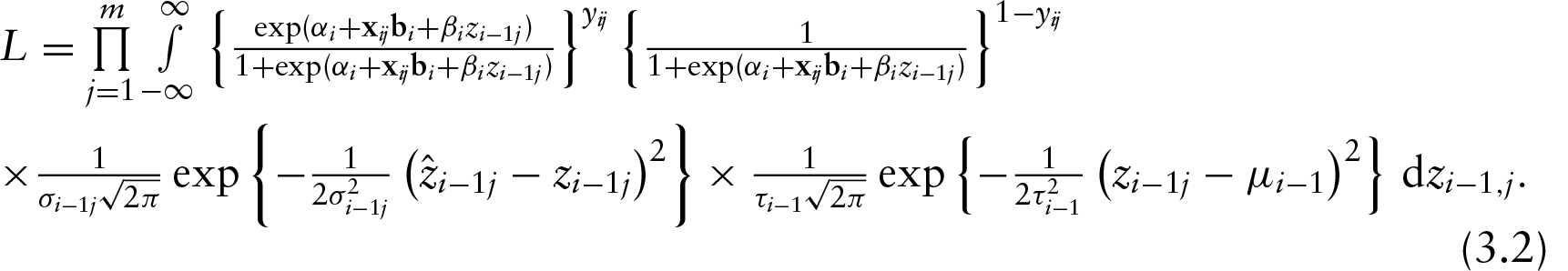
The likelihood approach maximizes the joint probability density $f (Y, \hat{Z} | X)$ . We will assume a classical non-differential measurement error, which is appropriate if the errors do not contain extra information about the outcome (Carroll et al., 2006). This is a reasonable assumption because the error is in the score, which is the linear predictor from a generalized linear regression model developed at the previous stage and is, hence, not correlated with the outcome at the current stage. The joint density at stage $i > 1$ can be written as an integral containing three components (Carroll et al., 2006):

f (Y, {\hat{Z}}_{i - 1} | X_{i}) = \int f (Y | Z_{i - 1}, X_{i}) f ({\hat{Z}}_{i - 1} | Z_{i - 1}) f (Z_{i - 1} | X_{i}) {dZ}_{i - 1} .

(3.1)

This equation contains three components, and therefore three sub-models are required to specify the full likelihood. These are:

The outcome sub-model $f (Y | Z_{i - 1}, X_{i})$ : This is just a GLM. For logistic regression (and, therefore, sequential logistic measurement error regression), we set

prob (y_{j} = 1 | z_{i - 1 j}, x_{ij}) = \frac{exp (α_{i} + x_{ij} b_{i} + β_{i} z_{i - 1 j})}{1 + exp (α_{i} + x_{ij} b_{i} + β_{i} z_{i - 1 j})},

and

prob (y_{j} = 0 | z_{i - 1 j}, x_{ij}) = 1 - prob (y_{j} = 1 | z_{i - 1 j}, x_{ij})

. For Poisson log-linear regression (and, therefore, sequential Poisson log-linear measurement error regression), we set

prob (y_{j} = y | z_{i - 1 j}, x_{ij}) = exp \{y (α_{i} + x_{ij} b_{i} + β_{i} z_{i - 1 j}) - e^{(α_{i} + x_{ij} b_{i} + β_{i} z_{i - 1 j})}\} / y!

(y = 0, 1, . . .)

. For linear regression (normal errors), we set

f (y_{j} | z_{i - 1 j}, x_{ij}) = \frac{1}{η \sqrt{2 π}} exp [- \frac{1}{2 η^{2}} {\{y_{j} - (α_{i} + x_{ij} b_{i} + β_{i} z_{i - 1 j})\}}^{2}] .

The measurement error sub-model $f ({\hat{Z}}_{i - 1} | Z_{i - 1})$ : The classical additive measurement error model, ${\hat{z}}_{i - 1 j} = z_{i - 1 j} + u_{ij}$ , is assumed (Carroll et al., 2006), where $u_{ij}$ is the additive normally distributed error so that $f ({\hat{Z}}_{i - 1} | Z_{i - 1}) = N (0, σ_{i - 1 j}^{2})$ . The assumption of normality is reasonable, since the score is a linear sum of parameters, each having an associated uncertainty.

The sub-model for the true unknown score $f (Z_{i - 1} | X_{i})$ : This sub-model can be difficult to specify in general and, therefore, can have a considerable impact on model robustness. The score $Z_{i - 1}$ , however, is the linear predictor from a GLM which is asymptotically normally distributed (McCullagh and Nelder, 1989) and, therefore, $z_{i - 1 j} \sim N (μ_{i - 1}, τ_{i - 1}^{2})$ . For the application which was used in this article, it was reasonable to assume that $Z_{i - 1}$ is independent of $X_{i}$ (see Section 4 for further details). Therefore, this sub-model becomes $f (Z_{i - 1})$ . This assumption will not be valid for all applications, but for this work, we will continue by assuming that $Z_{i - 1}$ is independent of $X_{i}$ .

For sequential logistic measurement error regression, the likelihood function is then

\begin{matrix} L = \prod_{j = 1}^{m} \int_{- \infty}^{\infty} {\{\frac{exp (α_{i} + x_{ij} b_{i} + β_{i} z_{i - 1 j})}{1 + exp (α_{i} + x_{ij} b_{i} + β_{i} z_{i - 1 j})}\}}^{y_{ij}} {\{\frac{1}{1 + exp (α_{i} + x_{ij} b_{i} + β_{i} z_{i - 1 j})}\}}^{1 - y_{ij}} \\ \times \frac{1}{σ_{i - 1 j} \sqrt{2 π}} exp \{- \frac{1}{2 σ_{i - 1 j}^{2}} {({\hat{z}}_{i - 1 j} - z_{i - 1 j})}^{2}\} \times \frac{1}{τ_{i - 1} \sqrt{2 π}} exp \{- \frac{1}{2 τ_{i - 1}^{2}} {(z_{i - 1 j} - μ_{i - 1})}^{2}\} d z_{i - 1, j} . \end{matrix}

(3.2)

The process of maximizing this likelihood function with respect to parameter vector $[α_{i}, b_{i}, β_{i}, μ_{i - 1}, τ_{i - 1}^{2}]$ requires some technical, numerical work, and this is discussed in the next sub-section. Higdon and Schafer (2001) discuss the identifiability of such measurement error models. They point out that even when the model is identifiable (e.g., when sub-model 1 is logistic regression and sub-models 2 and 3 are normal), there is no practical information contained in the parameter estimates without validation or replication data; hence, the measurement error variance $σ_{i - 1 j}^{2}$ should be known.

3.3.2 Fitting the sequential measurement error model

The steps required to fit the sequential measurement error model are as follows:

The measurement error variance is estimated using bootstrap samples.

The estimated score is calculated from the model at the previous stage.

The likelihood is evaluated numerically using Gauss—Hermite quadrature.

The log-likelihood is maximized using the Newton—Raphson method.

These steps are discussed further below:

Step 1: In the first step, the measurement error variance for the observed score at the previous stage is calculated for each observation. A number of methods have been suggested for this calculation: (a) via a validation dataset (e.g., Guo and Little, 2011), where the true score is actually observed; (b) using replicate measurements of ${\hat{z}}_{i - 1 j};$ (e.g., Rabe-Hesketh et al. 2003; and (c) via an instrument variable (e.g., Rosner et al., 1990). In the example that we describe later, neither a validation dataset nor replicate measurements nor an instrument variable were available. Therefore, we recommend to use bootstrap samples of the original data to obtain replicated values of the estimated scores, that is, to refit the model at the previous stage using the bootstrap sample and to use the bootstrap sample variance of these estimated scores (Efron and Tibshirani, 1993).

Step 2: At each stage, the estimated scores ${\hat{Z}}_{i - 1}$ must be calculated for each observation. At the first stage, this is a null step as there is no previous stage. At the second stage, we can use ${\hat{z}}_{1 j} = g {E (y_{j} | x_{1 j})} = {\hat{α}}_{1} + x_{1 j} {\hat{b}}_{1}$ , where ${\hat{α}}_{1}, {\hat{b}}_{1}$ are the estimates from the first stage and g is the link function in the GLM, since there is no measurement error component in the model fitted at the first stage. At the third stage, matters are more complicated. To quantify all predictive information from a previous stage in which there is a measurement error component, the estimated score is obtained from $g {E (y_{j} | {\hat{z}}_{i - 1 j}, x_{ij})}$ evaluated at the maximum likelihood estimate. Conceptually, this is the linearized predicted outcome from the previous stage and is calculated as follows. First, we have to calculate the probability density of $y_{j} | {\hat{z}}_{i - 1 j}, x_{ij}$ :

f (y_{j} | {\hat{z}}_{i - 1 j}, x_{ij}) = \frac{f (y_{j}, {\hat{z}}_{i - 1 j} | x_{ij})}{\int f (y, {\hat{z}}_{i - 1 j} | x_{ij}) d y},

(3.3)

then evaluate its expectation and finally transform the result using g. When the outcome variable is discrete, then the integral in the denominator of Equation (3.3) is a summation. In the case of logistic regression,

g {E (y_{j} | {\hat{z}}_{i - 1 j}, x_{ij})}

is the logit transform of the fitted success probability: the fitted success probability is

f (y_{j} = 1 | {\hat{z}}_{i - 1 j}, x_{ij}) = \frac{f (y_{j} = 1, {\hat{z}}_{i - 1 j} | x_{ij})}{f (y_{j} = 1, {\hat{z}}_{i - 1 j} | x_{ij}) + f (y_{j} = 0, {\hat{z}}_{i - 1 j} | x_{ij})},

(3.4)

so that

g {E (y_{j} | {\hat{z}}_{i - 1 j}, x_{ij})} = log {\frac{f (y_{j} = 1 | {\hat{z}}_{i - 1 j}, x_{ij})}{1 - f (y_{j} = 1 | {\hat{z}}_{i - 1 j}, x_{ij})}} .

The terms in the right-hand side of Equation (3.4) are evaluated in the same way as the likelihood function (3.1; described next) and setting parameters equal to their maximum likelihood estimates.

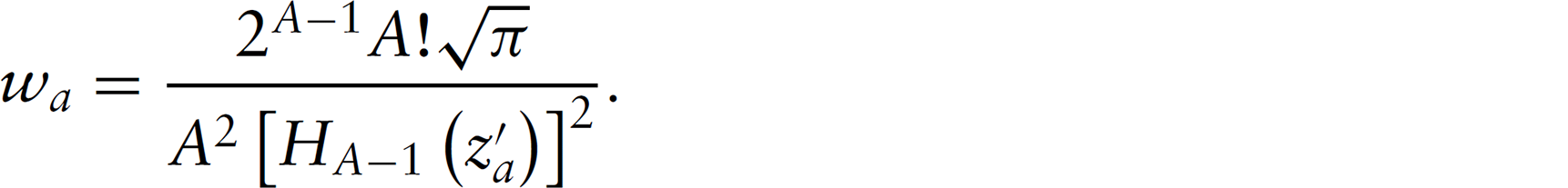
Step 3: The likelihood is evaluated numerically using, for example, Gauss—Hermite quadrature (Hildebrand, 1974), which is an ideal technique for approximating integrals involving exponentials as follows:

\int_{- \infty}^{+ \infty} e^{- z^{' 2}} f (z^{'}) {dz}^{'} ≅ \sum_{a = 1}^{A} w_{a} f (z_{a}^{'}),

where A is the number of sample points used for the approximation,

z_{a}^{'}

are the roots of the Hermite polynomial

H_{A} (z^{'})

and

w_{a}

are the associated weights given by

w_{a} = \frac{2^{A - 1} A! \sqrt{π}}{A^{2} {[H_{A - 1} (z_{a}^{'})]}^{2}} .

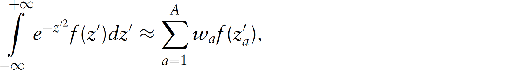
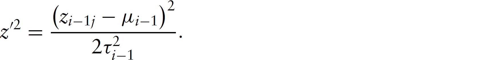
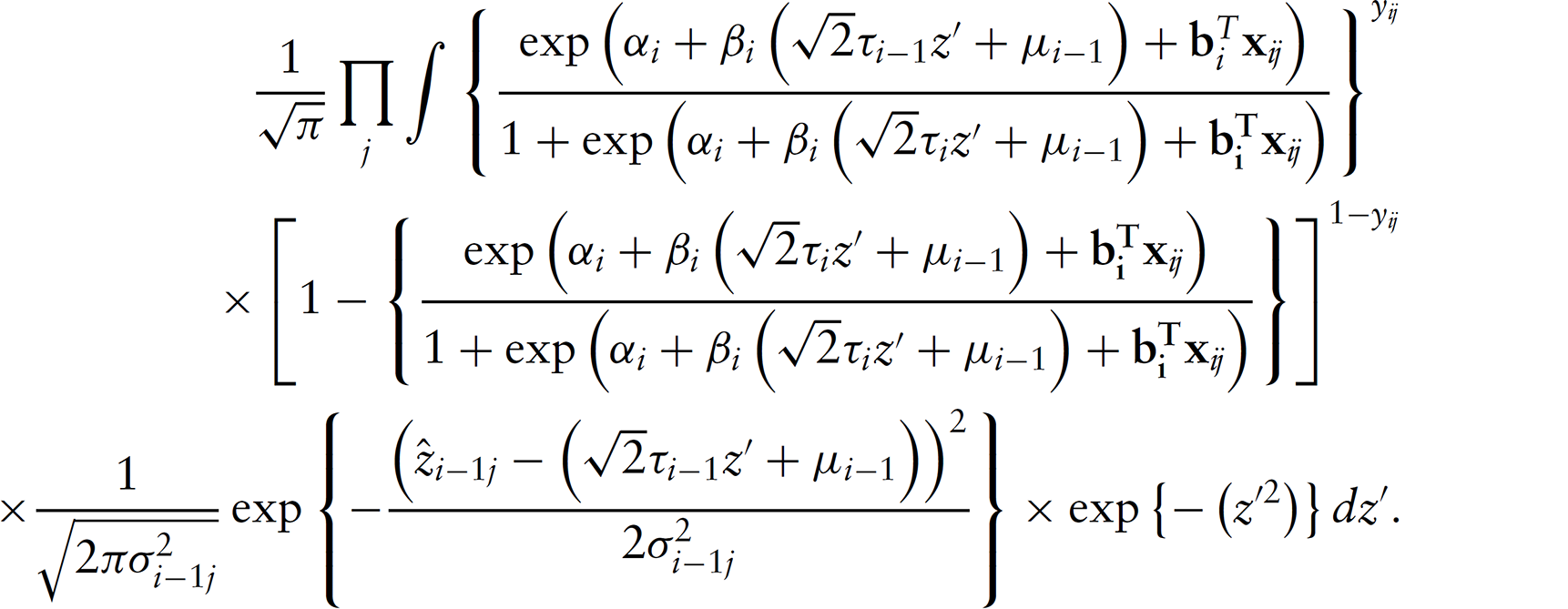
In order to apply Gauss—Hermite quadrature, the likelihood of Equation (3.2) needs to be transformed to the correct form by defining $z^{' 2}$ as follows:

z^{' 2} = \frac{{(z_{i - 1 j} - μ_{i - 1})}^{2}}{2 τ_{i - 1}^{2}} .

The likelihood (Equation 3.2) can then be written as

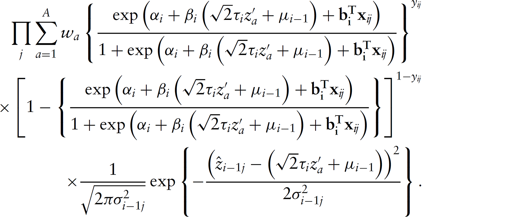
\begin{matrix} \frac{1}{\sqrt{π}} \prod_{j} \int {\{\frac{exp (α_{i} + β_{i} (\sqrt{2} τ_{i - 1} z^{'} + μ_{i - 1}) + b_{i}^{T} x_{ij})}{1 + exp (α_{i} + β_{i} (\sqrt{2} τ_{i} z^{'} + μ_{i - 1}) + b_{i}^{T} x_{ij})}\}}^{y_{ij}} \\ \times {[1 - \{\frac{exp (α_{i} + β_{i} (\sqrt{2} τ_{i} z^{'} + μ_{i - 1}) + b_{i}^{T} x_{ij})}{1 + exp (α_{i} + β_{i} (\sqrt{2} τ_{i} z^{'} + μ_{i - 1}) + b_{i}^{T} x_{ij})}\}]}^{1 - y_{ij}} \\ \times \frac{1}{\sqrt{2 π σ_{i - 1 j}^{2}}} exp \{- \frac{{({\hat{z}}_{i - 1 j} - (\sqrt{2} τ_{i - 1} z^{'} + μ_{i - 1}))}^{2}}{2 σ_{i - 1 j}^{2}}\} \times exp \{- (z^{' 2})\} {dz}^{'} . \end{matrix}

This is now in the form of Gauss—Hemite quadrature and can be approximated numerically as

\begin{matrix} \prod_{j} \sum_{a = 1}^{A} w_{a} {\{\frac{exp (α_{i} + β_{i} (\sqrt{2} τ_{i} z_{a}^{'} + μ_{i - 1}) + b_{i}^{T} x_{ij})}{1 + exp (α_{i} + β_{i} (\sqrt{2} τ_{i} z_{a}^{'} + μ_{i - 1}) + b_{i}^{T} x_{ij})}\}}^{y_{ij}} \\ \times {[1 - \{\frac{exp (α_{i} + β_{i} (\sqrt{2} τ_{i} z_{a}^{'} + μ_{i - 1}) + b_{i}^{T} x_{ij})}{1 + exp (α_{i} + β_{i} (\sqrt{2} τ_{i} z_{a}^{'} + μ_{i - 1}) + b_{i}^{T} x_{ij})}\}]}^{1 - y_{ij}} \\ \times \frac{1}{\sqrt{2 π σ_{i - 1 j}^{2}}} exp \{- \frac{{({\hat{z}}_{i - 1 j} - (\sqrt{2} τ_{i} z_{a}^{'} + μ_{i - 1}))}^{2}}{2 σ_{i - 1 j}^{2}}\} . \end{matrix}

Step 4: For computational purposes, it is easier to work with the log-likelihood. The accuracy of the quadrature depends on the number of points selected. We recommend evaluating the log-likelihood for increasing number of points starting with 10 in steps of 10 until a required accuracy is attained. The log-likelihood is then maximized to determine the unknown parameters, using, for example, Newton—Raphson method (Collett (2002)), which has been found to work well for measurement error models Rabe-Hesketh et al. (2003). We recommend using the fitted values from the sequential regression as initial values for ${\hat{α}}_{i}$ , ${\hat{b}}_{i}$ , ${\hat{β}}_{i}$ in the maximization procedure for stage $i = 2$ . For stages $i > 2$ , the sequential regression model can be refitted using the estimated score as calculated at Step 2 to yield initial values. The mean and standard deviation of ${\hat{z}}_{i - 1 j}$ over all j observations provide initial values for $μ_{i - 1}$ and $τ_{i - 1}$ . Standard errors are obtained from the variance–covariance matrix. This can be approximated by the negative inverse of the Hessian matrix (the matrix of the second derivatives of the log-likelihood with respect to the unknown parameters) which is obtained from the final stage of the Newton–Rapshon process. The p-values are then calculated in the same way as for normal logistic regression.

At each stage, one would expect to carry out a variable reduction procedure, proceeding in the same way as for the sequential regression model, Section 3.2.

4 Example: The match sprint in track cycling

We now illustrate our ideas using an example from sport: the match sprint in track cycling. This is a highly tactical race that takes place between two riders in a velodrome. In major competitions, the riders race over three laps of a 250 m track. They start together and the first across the finish line wins. In major competitions, the event is organized in knock-out rounds, each round being a best-of-three race. An initial qualifying round, in which riders race individually against the clock over a ‘flying’ 200 m, determines the qualifiers and pairings for the knock-out rounds. The time an individual sets in the flying 200 m is called the ‘flying time’ and the implied speed the ‘flying speed’: This is an important covariate that we will use later. More details of the event can be found with UCI (2016). As the outcome of a single race is win or loss, we use logistic regression. Now, we want to (a) compare the ‘novel sequential logistic measurement error regression’ (Model 3) with ‘naïve sequential logistic regression’ (Model 1) and ‘sequential logistic regression’ (Model 2) and (b) briefly describe some tactical implications for riders and coaches that our preferred model suggests.

The factors that determine the outcome of a race are described in the next sub-section. We then present our results and compare and contrast the three models.

4.1 Factors in the match sprint: Description and data collection

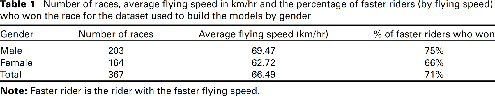
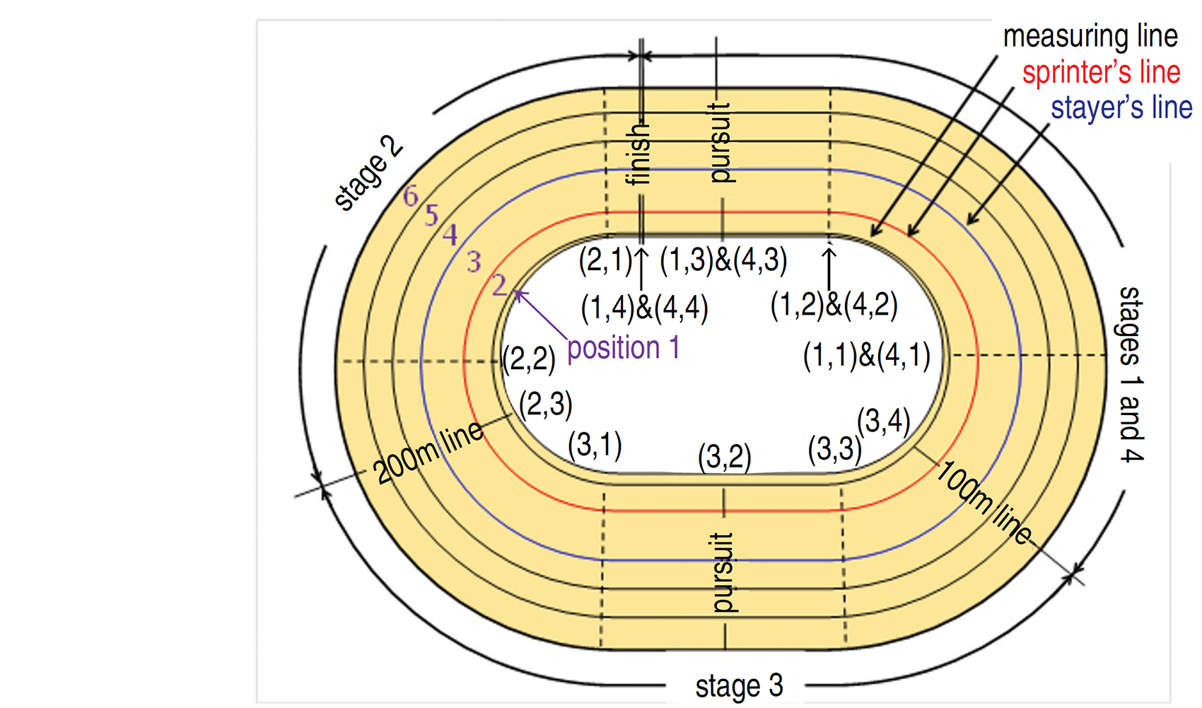
Using video footage, supplied by British Cycling, of 367 races from major competitions between 2006 and 2008 (see Table 1), the times and the position (perpendicular distance from the inside of the track) at which riders crossed each of the five visible marks (the solid longitudinal lines shown in Figure 1) for each of the races were found. Times were determined to an accuracy of 1/50th second. Positions were ordinally categorized and were also collected at each mark and each virtual mark as shown in Figure 1 (11 marks in total). The track is not flat but slopes upwards, linearly from the inside. The slope is greatest at the apex of the curves. Using the known three-dimensional geometry of the track and the information collected from video footage, riders’ average speeds over a stage were estimated; this is discussed further in Moffatt et al. (2014). The flying speeds of riders from the qualifying round were obtained from the Tissot Timing website (Tissot Timing, 2016). The average flying speeds were 63 km/hr and 69 km/hr for female and male riders, respectively (see Table 1).

Table 1 :

Number of races, average flying speed in km/hr and the percentage of faster riders (by flying speed) who won the race for the dataset used to build the models by gender

Gender	Number of races	Average flying speed (km/hr)	% of faster riders who won
Male	203	69.47	75%
Female	164	62.72	66%
Total	367	66.49	71%

Note: Faster rider is the rider with the faster flying speed.

Figure 1:

Plan view of a track, showing the track division for determining speed and position and describing covariates and tactics: The latitudinal lines divide the track into six positions. The Finish, 200 m and 100 m, lines divide the track into stages, with stage 1 occurring in lap 1 and stages 2–4 occurring in lap 2. The diagram also shows the marks on the track at which data were collected, which correspond to either actual markings on the track (– –), or to virtual marks (—) where additional information regarding riders’ positions was collected. Each mark is given a label comprising two numbers: The first number refers to the stage and the second refers to the mark within the stage.

The faster rider (rider with the faster flying speed) does not always win; in the dataset used to build the model, the faster rider won 71 $%$ of the time (see Table 1). The race is, therefore, highly tactical; broadly speaking, riders vie for track position in the first part of the race and sprint for the finish line in the second part. Riders typically cannot sustain an early sprint; flat out sprints from the start are rare and will be unsuccessful unless the trailing rider is taken by surprise or is much weaker. Therefore, throughout a race, a rider must make decisions about speed and position based upon an opponent's speed and position, distance to the finish, and pre-race tactical plans.

In each model (1–3), we assign the reference rider as the faster rider by ‘flying speed’, and the outcome is recorded from the point of view of this rider. For modelling, we divide the race into the following stages as shown in Figure 1. Stage 1 is the last 100 m of the first lap (600 m to 500 m to go). Moffatt et al. (2014) found race tactics not to be important prior to 600 m to go; therefore, this part of the race was not considered. At the end of stage 1, there are two laps (500 m) to go. Stage 2 is the next 50 m, stage 3 is the next 100 m and stage 4 is the final 100 m of the second lap (see Figure 1). Thus, four regressions are fitted at 500 m, 450 m, 350 m and 250 m to go. Tactically, the second lap is the crux of the race, and riders are committed to their actions as they enter the final lap: sprinting flat-out to hold the lead while staying inside the sprinter's line or slipstreaming and overtaking around the final bend.

4.2 Model fitting procedure

Model 1 was fitted using the standard functions available in the R programming language (R Development Core Team, 2016). The fitting of Models 2 and 3 was implemented in MATLAB $®$ (2007, Mathworks, Natick, Massachusetts), including the variable selection procedure. The final set of covariates described in Tables 2 and 3, which includes first order interactions, was developed from the primary covariates (positions and average speeds). The final set of covariates relates to the average speed of the riders over stages, track position at the marks, changes of position and changes of lead (overtaking). In this example, over 30 covariates were considered at each stage. This made it impractical to use a variable selection technique which involved fitting all possible regressions and choosing between them using, for example, Akaike information criterion or Bayesian information criterion (Dobson and Barnett, 2008). Instead, a procedure using bootstrap techniques in conjunction with forward stepwise was used (Sauerbrei and Schumacher, 1992). This involved generating bootstrap samples and fitting the regression to each bootstrap sample using forward stepwise to yield a bootstrap regression for each member of the bootstrap sample. Revealed covariates are selected for the final regression based on the number of times they appear in the bootstrap regressions. Although this procedure has been criticized for misselection (Austin (2008)), the broad view is that it selects covariates robustly.

As discussed in Section 3.3.1, for this application we assume that $Z_{i - 1}$ is independent of $X_{i}$ . This means that the true score (which is related to the probability of winning at the previous stage) is not correlated with the other covariates revealed in the current stage. This assumption was tested on our dataset by testing for correlation between the estimated score and the other covariates for the final model. Pearson product-moment correlation coefficient was calculated between the estimated score and the other covariates. No significant correlation (p-value less than 0.05) was found, indicating that this is also likely to be valid for the true score.

In order to directly compare Models 1 to 3, the same sets of covariates were used. These covariates were selected when applying the sequential model (Model 2) rather than the measurement error model (Model 3). This approach is likely to be more stringent because the sequential regression model is more optimistic about the size of effects, and this approach also had the advantage of reducing the computational burden (Moffatt, 2012).

4.3 Results

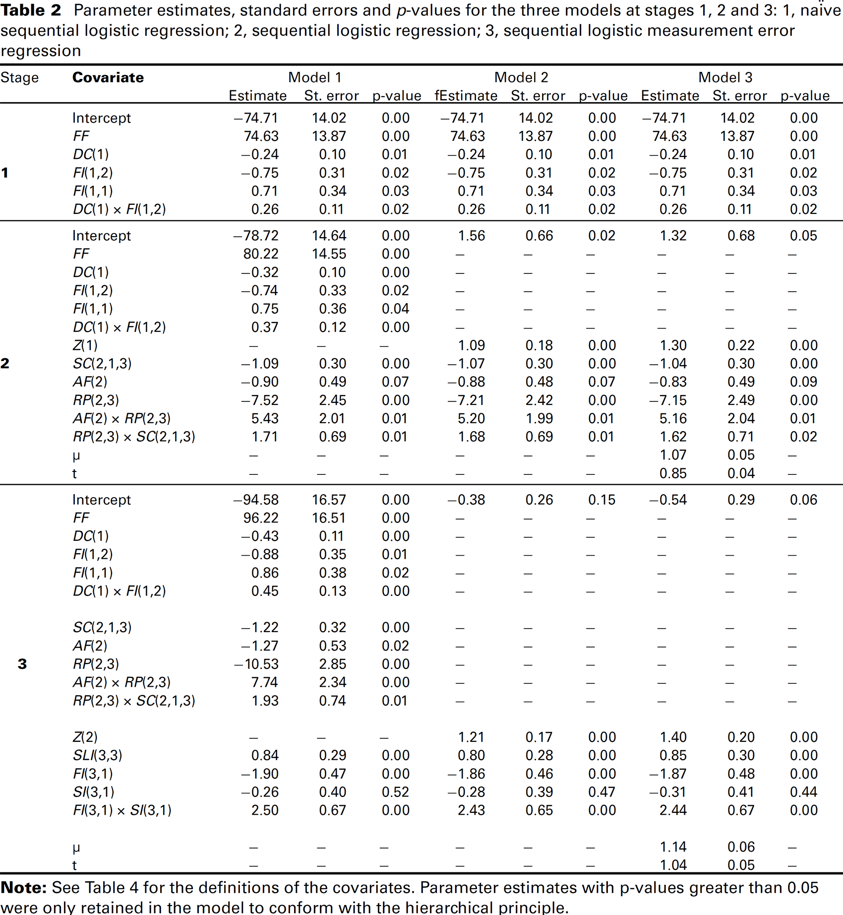
Tables 2 and 3 show how the interpretative complexity of the naïve sequential regression (Model 1) increases through the stages. The parameter estimates are generally more significant and the standard errors are generally larger for the naïve sequential model (Model 1). There are many more covariates in the naïve sequential models; therefore, there are not as many events (event being the outcome which occurred less often, i.e., win or lose in this case) per covariate term. Even at 450 m to go, there are only nine events per covariate term, reducing to five events per covariate term at 250 m to go. This suggests that the naïve sequential models in general are likely to be unstable/poorly estimated at later stages, particularly when there are many covariates in the models. Peduzzi et al. (1996) found in a simulated study that the variability in the parameter estimates becomes large and, hence, inaccurate when there are less than 10 events per covariate.

Table 2:

Parameter estimates, standard errors and p-values for the three models at stages 1, 2 and 3: 1, naïve sequential logistic regression; 2, sequential logistic regression; 3, sequential logistic measurement error regression.

Stage	Covariate	Model 1			Model 2			Model 3
		Estimate	St. error	p-value	Estimate	St. error	p-value	Estimate	St. error	p-value
	Intercept	-74.71	14.02	0.00	-74.71	14.02	0.00	-74.71	14.02	0.00
	FF	74.63	13.87	0.00	74.63	13.87	0.00	74.63	13.87	0.00
	DC(1)	-0.24	0.10	0.01	-0.24	0.10	0.01	-0.24	0.10	0.01
1	FI(1,2)	-0.75	0.31	0.02	-0.75	0.31	0.02	-0.75	0.31	0.02
	FI(1,1)	0.71	0.34	0.03	0.71	0.34	0.03	0.71	0.34	0.03
	DC(1) Õ FI(1,2)	0.26	0.11	0.02	0.26	0.11	0.02	0.26	0.11	0.02
	Intercept	-78.72	14.64	0.00	1.56	0.66	0.02	1.32	0.68	0.05
	FF	80.22	14.55	0.00	-	-	-	-	-	-
	DC(1)	-0.32	0.10	0.00	-	-	-	-	-	-
	FI(1,2)	-0.74	0.33	0.02	-	-	-	-	-	-
	FI(1,1)	0.75	0.36	0.04	-	-	-	-	-	-
	DC(1) Õ FI(1,2)	0.37	0.12	0.00	-	-	-	-	-	-
	Z(1)	-	-	-	1.09	0.18	0.00	1.30	0.22	0.00
2	SC(2,1,3)	-1.09	0.30	0.00	-1.07	0.30	0.00	-1.04	0.30	0.00
	AF(2)	-0.90	0.49	0.07	-0.88	0.48	0.07	-0.83	0.49	0.09
	RP(2,3)	-7.52	2.45	0.00	-7.21	2.42	0.00	-7.15	2.49	0.00
	AF(2) Õ RP(2,3)	5.43	2.01	0.01	5.20	1.99	0.01	5.16	2.04	0.01
	RP(2,3) Õ SC(2,1,3)	1.71	0.69	0.01	1.68	0.69	0.01	1.62	0.71	0.02
	Μ	-	-	-	-	-	-	1.07	0.05	-
	t	-	-	-	-	-	-	0.85	0.04	-
	Intercept	-94.58	16.57	0.00	-0.38	0.26	0.15	-0.54	0.29	0.06
	FF	96.22	16.51	0.00	-	-	-	-	-	-
	DC(1)	-0.43	0.11	0.00	-	-	-	-	-	-
	FI(1,2)	-0.88	0.35	0.01	-	-	-	-	-	-
	FI(1,1)	0.86	0.38	0.02	-	-	-	-	-	-
	DC(1) Õ FI(1,2)	0.45	0.13	0.00	-	-	-	-	-	-
	SC(2,1,3)	-1.22	0.32	0.00	-	-	-	-	-	-
	AF(2)	-1.27	0.53	0.02	-	-	-	-	-	-
3	RP(2,3)	-10.53	2.85	0.00	-	-	-	-	-	-
	AF(2) Õ RP(2,3)	7.74	2.34	0.00	-	-	-	-	-	-
	RP(2,3) Õ SC(2,1,3)	1.93	0.74	0.01	-	-	-	-	-	-
	Z(2)	-	-	-	1.21	0.17	0.00	1.40	0.20	0.00
	SLI(3,3)	0.84	0.29	0.00	0.80	0.28	0.00	0.85	0.30	0.00
	FI(3,1)	-1.90	0.47	0.00	-1.86	0.46	0.00	-1.87	0.48	0.00
	SI(3,1)	-0.26	0.40	0.52	-0.28	0.39	0.47	-0.31	0.41	0.44
	FI(3,1) Õ SI(3,1)	2.50	0.67	0.00	2.43	0.65	0.00	2.44	0.67	0.00
	Μ	-	-	-	-	-	-	1.14	0.06	-
	t	-	-	-	-	-	-	1.04	0.05	-

Note: See Table 4 for the definitions of the covariates. Parameter estimates with p-values greater than 0.05 were only retained in the model to conform with the hierarchical principle.

Table 3 :

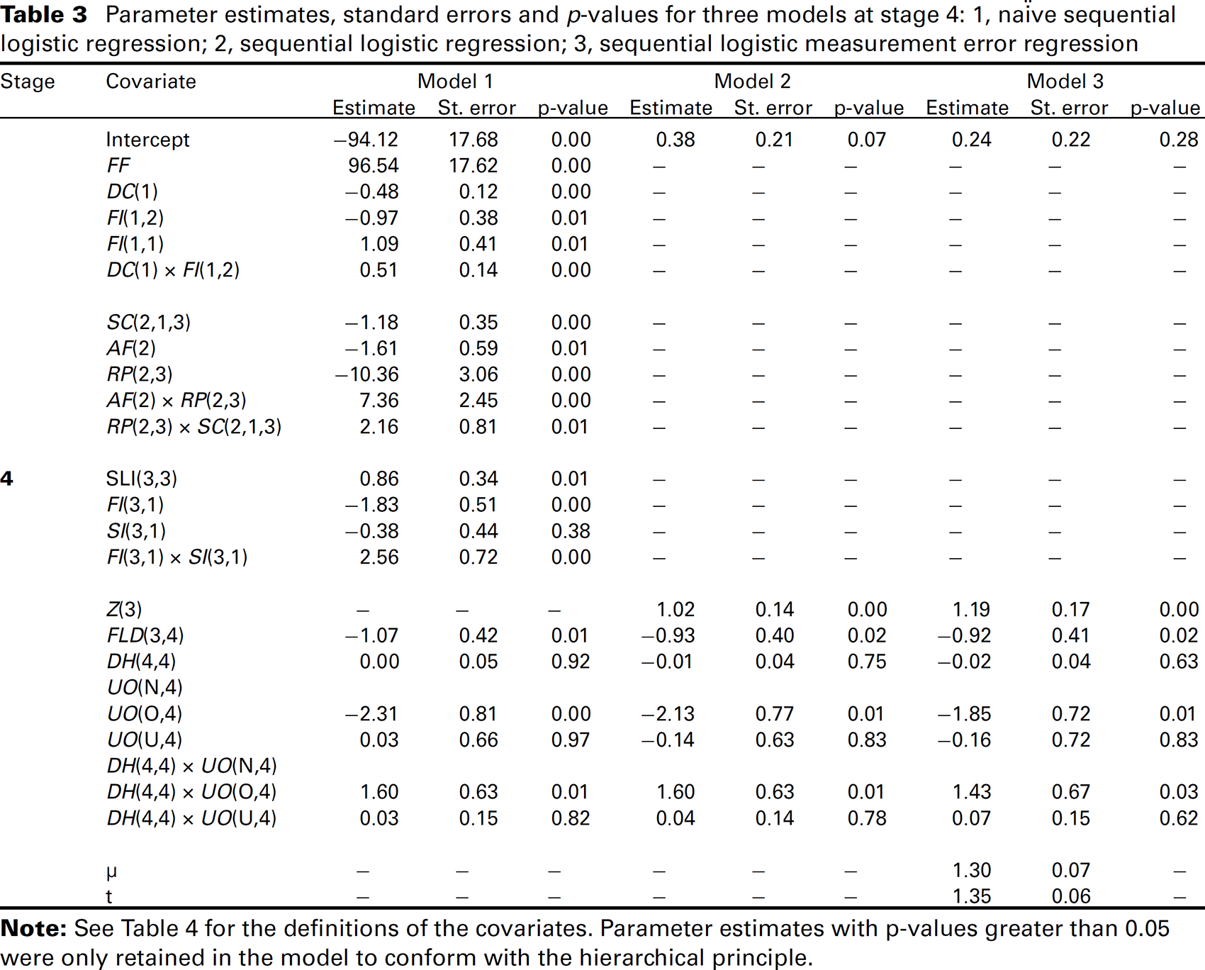
Parameter estimates, standard errors and p-values for three models at stage 4: 1, naïve sequential logistic regression; 2, sequential logistic regression; 3, sequential logistic measurement error regression.

Stage	Covariate	Model 1			Model 2			Model 3
		Estimate	St. error	p-value	Estimate	St. error	p-value	Estimate	St. error	p-value
	Intercept	-94.12	17.68	0.00	0.38	0.21	0.07	0.24	0.22	0.28
	FF	96.54	17.62	0.00	-	-	-	-	-	-
	DC(1)	-0.48	0.12	0.00	-	-	-	-	-	-
	FI(1,2)	-0.97	0.38	0.01	-	-	-	-	-	-
	FI(1,1)	1.09	0.41	0.01	-	-	-	-	-	-
	DC(1) Õ FI(1,2)	0.51	0.14	0.00	-	-	-	-	-	-
	SC(2,1,3)	-1.18	0.35	0.00	-	-	-	-	-	-
	AF(2)	-1.61	0.59	0.01	-	-	-	-	-	-
	RP(2,3)	-10.36	3.06	0.00	-	-	-	-	-	-
	AF(2) Õ RP(2,3)	7.36	2.45	0.00	-	-	-	-	-	-
	RP(2,3) Õ SC(2,1,3)	2.16	0.81	0.01	-	-	-	-	-	-
4	SLI(3,3)	0.86	0.34	0.01	-	-	-	-	-	-
	FI(3,1)	-1.83	0.51	0.00	-	-	-	-	-	-
	SI(3,1)	-0.38	0.44	0.38	-	-	-	-	-	-
	FI(3,1) Õ SI(3,1)	2.56	0.72	0.00	-	-	-	-	-	-
	Z(3)	-	-	-	1.02	0.14	0.00	1.19	0.17	0.00
	FLD(3,4)	-1.07	0.42	0.01	-0.93	0.40	0.02	-0.92	0.41	0.02
	DH(4,4)	0.00	0.05	0.92	-0.01	0.04	0.75	-0.02	0.04	0.63
	UO(N,4)
	UO(O,4)	-2.31	0.81	0.00	-2.13	0.77	0.01	-1.85	0.72	0.01
	UO(U,4)	0.03	0.66	0.97	-0.14	0.63	0.83	-0.16	0.72	0.83
	DH(4,4) Õ UO(N,4)
	DH(4,4) Õ UO(O,4)	1.60	0.63	0.01	1.60	0.63	0.01	1.43	0.67	0.03
	DH(4,4) Õ UO(U,4)	0.03	0.15	0.82	0.04	0.14	0.78	0.07	0.15	0.62

	Μ	-	-	-	-	-	-	1.30	0.07	-
	t	-	-	-	-	-	-	1.35	0.06	-

Note: See Table 4 for the definitions of the covariates. Parameter estimates with p-values greater than 0.05 were only retained in the model to conform with the hierarchical principle.

Table 4:

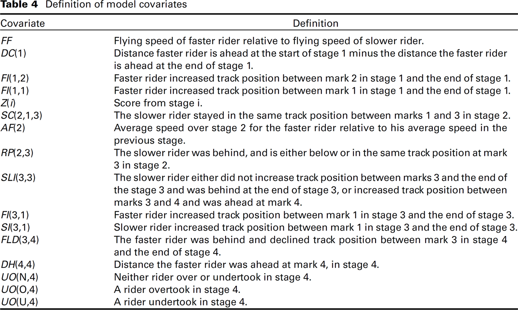
Definition of model covariates

Covariate	Definition
FF	Flying speed of faster rider relative to flying speed of slower rider.
DC(1)	Distance faster rider is ahead at the start of stage 1 minus the distance the faster rider is ahead at the end of stage 1.
FI(1,2)	Faster rider increased track position between mark 2 in stage 1 and the end of stage 1.
FI(1,1)	Faster rider increased track position between mark 1 in stage 1 and the end of stage 1.
Z(i)	Score from stage i.
SC(2,1,3)	The slower rider stayed in the same track position between marks 1 and 3 in stage 2.
AF(2)	Average speed over stage 2 for the faster rider relative to his average speed in the previous stage.
RP(2,3)	The slower rider was behind, and is either below or in the same track position at mark 3 in stage 2.
SLI(3,3)	The slower rider either did not increase track position between marks 3 and the end of the stage 3 and was behind at the end of stage 3, or increased track position between marks 3 and 4 and was ahead at mark 4.
FI(3,1)	Faster rider increased track position between mark 1 in stage 3 and the end of stage 3.
SI(3,1)	Slower rider increased track position between mark 1 in stage 3 and the end of stage 3.
FLD(3,4)	The faster rider was behind and declined track position between mark 3 in stage 4 and the end of stage 4.
DH(4,4)	Distance the faster rider was ahead at mark 4, in stage 4.
UO(N,4)	Neither rider over or undertook in stage 4.
UO(O,4)	A rider overtook in stage 4.
UO(U,4)	A rider undertook in stage 4.

The sequential regression (Model 2) reduces this complexity; however, as discussed in Section 3, the sequential model assumes that the estimated score is measured without error, which is not true. When accounting for error in the score (Model 3) with a well-established measurement error method for our dataset, the estimated effect of the score at each stage is between 16% and 19% higher than when not accounting for error in the score (Model 2). This indicates that not accounting for the error in the score can lead to the estimate of the effect of the true unknown score being biased towards zero. The parameter estimates for most of the revealed covariates are similar for the sequential and sequential measurement error models. Therefore, the effect of the actions riders apply on win probability at each stage is similar for the sequential and sequential measurement error models. The key actions and race states that appear to influence race outcome at each stage are described in the next sub-section. However, the sequential model which underestimates the effect of the true unknown score, therefore, conversely overestimates the effects of revealed covariates. In this way, the sequential model places more importance on race actions and less on the ratio of flying speeds (the covariate that dominates the score) than the sequential measurement error model.

The parameter estimates which are most dissimilar for the sequential and sequential measurement error models are UO(O,4) and DH(4,4) $\times$ UO(O,4) in the 250 m to go model. The sequential model most likely overestimates these two terms because there are few instances where riders overtake at this stage. The measurement error technique, therefore, reduces this likely overestimation. The standard errors for the parameter estimates are slightly larger for the sequential measurement error models, as would be expected because the measurement error variance implies greater uncertainty in the estimation process.

Accounting for the error in the score also led to differences in the predicted win probabilities, which generally increase with the stage. At 450 m to go, for the majority of races, these differences are within the range $-$ 0.02 and 0.02, with 308 (87%) races being within this range (see Table 5). At 350 m to go and 250 m to go, 114 (32%) and 127 (36%) races have an absolute difference greater than 0.02, respectively (see Table 5). This illustrates that in a sequential approach, the effects of measurement errors propagate through stages.

Table 5:

Number of races by the absolute difference in win probabilities for the faster rider at 450 m, 350 m and 250 m to go as predicted by the sequential and measurement error models.

Model	Difference in probability
	< = 0.01	0.01 – 0.02	0.02 – 0.03	0.03 – 0.04	0.04 – 0.05	0.05 – 0.1	>0.1
450 m to go	221	87	24	6	5	5	7
350 m to go	147	94	43	21	12	20	18
250 m to go	134	90	46	27	20	25	9

Note: At 450 m and 350 m to go 12 races and at 250 m to go 16 were excluded due to missing values.

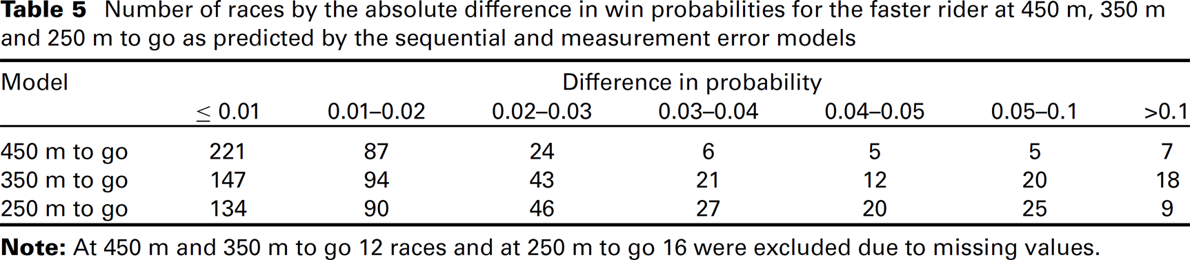
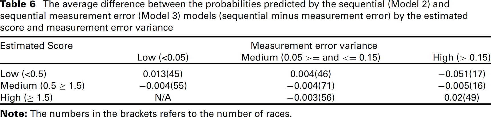
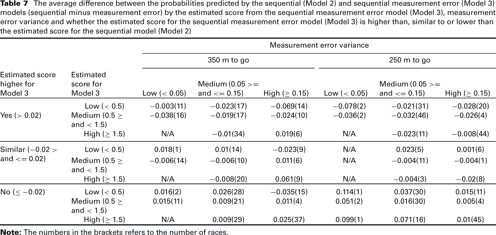
The differences in the probabilities predicted by the sequential and sequential measurement error models were investigated further. It was found that the model which predicted the higher probability of winning depends on the size of the measurement error variance as shown in Tables 6 and 7. When the measurement error variance is high and the estimated score is extreme (i.e., away from the median value), the sequential measurement error model predicts a less extreme win probability, as there is more uncertainty in the estimated score. An exception to this is when the estimated score for Model 3 is much more extreme than that for Model 2. Then, the sequential measurement error model predicts the more extreme probability (see Table 7 where the estimated score for Model 3 is more extreme and, at least, 0.02 lower). Overall, however, the measurement error model produces less extreme probabilities. A race which has an extremely high or low score at this stage of the race suggests that the outcome of the race has been decided. This seems very unlikely to be the case before 250 m to go and suggests that the extreme probabilities (less than 0.05 or greater than 0.95) predicted by the sequential model are questionable. For example, at 450 m to go, the riders are typically riding relatively slowly (around half of their maximum speed) and only around half of leading riders at this stage go on to win. Figure 2 shows an example of the effect a high measurement variance has on the difference in the predicted probabilities for a set of influential actions at 450 m to go for one particular race.

Table 6:

The average difference between the probabilities predicted by the sequential (Model 2) and sequential measurement error (Model 3) models (sequential minus measurement error) by the estimated score and measurement error variance

Estimated Score	Measurement error variance
	Low (<0.05)	Medium (0.5>= and <=0.15)	High (> = 0.15)
Low (<0.5)	0.013(45)	0.004(46)	$-$ 0.051(17)
Medium ( $0.5 \geq$ $1.5$ )	$-$ 0.004(55)	$-$ 0.004(71)	$-$ 0.005(16)
High ( $\geq 1.5$ )	N/A	$-$ 0.003(56)	0.02(49)

Note: The numbers in the brackets refers to the number of races.

Figure 2:

Win probability for the faster rider at 450 m to go (end of stage 2) as a function of AF(2), when SC(2,1,3) = 1 and RP(2,3) = 0 (see Table 4 for covariate definitions) for three cases with a low score Z(1), (–x–) = $-$ 0.12, (– –) = $-$ 0.38 and (– $•$ –)= $-$ 1.16, and with a low (0.05), medium (0.14) and high measurement error variance (0.67), respectively. Win probabilities are shown for the sequential model ( $\cdot$ $\cdot$ $\cdot$ ) and the (—) sequential measurement error model.

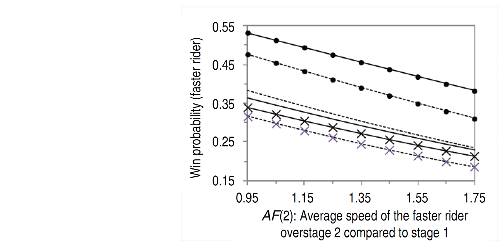
When the measurement error variance is low and the estimated score is extreme, the sequential measurement error model predicts a more extreme probability of winning for the faster rider, as there is more certainty in the estimated score. Tables 6 and 7 show the average difference predicted by the two models and Figure 2 shows an example of the effect a low measurement variance has on the predicted win probabilities for one race. The exception is when the estimated score for Model 3 is less extreme in comparison to the estimated score for Model 2. Then, the opposite becomes true in that the measurement error model predicts the less extreme probability. When the estimated score or measurement error variance is close to the median value (over all races), the win probabilities are similar at 450 m to go. At both 350 m and 250 m to go, when the estimated score for Model 3 is close to the median value, the difference in the win probabilities mostly depends on the difference between the estimated scores for Models 2 and 3.

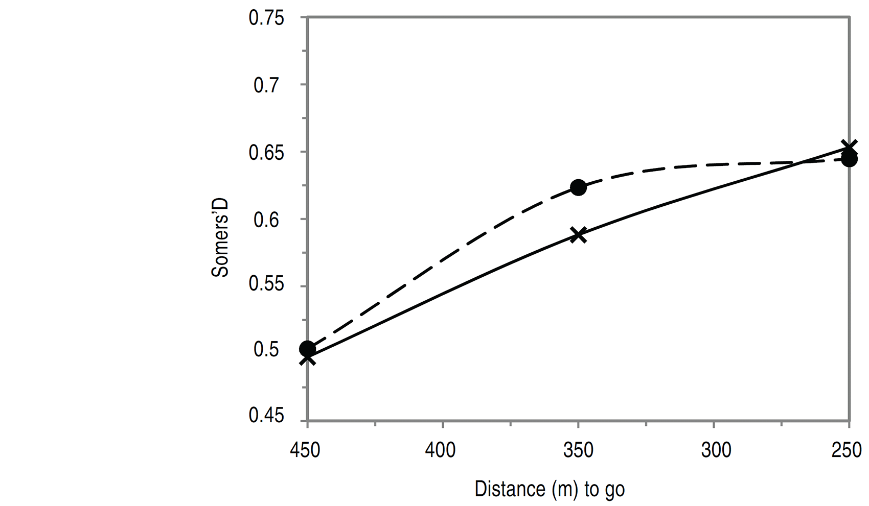
The fit of both Models 2 and 3 were compared by calculating the Somers’ D value, which is a measure of association between the observed and predicted responses. No extra data was available to test how well the models fit on a different dataset. Instead,

Table 7 :

The average difference between the probabilities predicted by the sequential (Model 2) and sequential measurement error (Model 3) models (sequential minus measurement error) by the estimated score from the sequential measurement error model (Model 3), measurement error variance and whether the estimated score for the sequential measurement error model (Model 3) is higher than, similar to or lower than the estimated score for the sequential model (Model 2).

	Measurement error variance
		350 m to go			250 m to go
Estimated score higher for Model 3	Estimated score for Model 3	Low (< 0.05)	Medium (0.5>= and <=0.15)	High ( $\geq$ 0.15)	Low (< 0.05)	Medium (0.5>= and <=0.15)	High ( $\geq$ 0.15)
	Low (< 0.5)	$-$ 0.003(11)	$-$ 0.023(17)	$-$ 0.069(14)	$-$ 0.078(2)	$-$ 0.021(31)	$-$ 0.028(20)
Yes (> 0.02)	Medium (0.5 $\geq$ and < 1.5)	$-$ 0.038(16)	$-$ 0.019(17)	$-$ 0.024(10)	$-$ 0.036(2)	$-$ 0.032(46)	$-$ 0.026(4)
	High ( $\geq$ 1.5)	N/A	$-$ 0.01(34)	0.019(6)	N/A	$-$ 0.023(11)	$-$ 0.008(44)
Similar (-0.02> and >=0.02)	Low (<0.5)	0.018(1)	0.01(14)	$-$ 0.023(9)	N/A	0.023(5)	0.001(6)
	Medium (0.5 $\geq$ and < 1.5)	$-$ 0.006(14)	$-$ 0.006(10)	0.011(6)	N/A	$-$ 0.004(11)	$-$ 0.004(1)
	High ( $\geq$ 1.5)	N/A	$-$ 0.008(20)	0.061(9)	N/A	$-$ 0.004(3)	$-$ 0.02(8)
No (< = 0.02)	Low (< 0.5)	0.016(2)	0.026(28)	$-$ 0.035(15)	0.114(1)	0.037(30)	0.015(11)
	Medium (0.5 $\geq$ and < 1.5)	0.015(11)	0.009(21)	0.011(4)	0.051(2)	0.016(30)	0.005(4)
	High ( $\geq$ 1.5)	N/A	0.009(29)	0.025(37)	0.099(1)	0.071(16)	0.01(45)

Note: The numbers in the brackets refers to the number of races.

the Somers’ D value was calculated on the same dataset used to the build model, but this value was adjusted using Efron's 0.682 estimator (Efron, 1983), which is used to adjust for the over-optimism in a Somers’ D value which is calculated based on the dataset used to fit the model. The Somers’ D value was similar for both the sequential and sequential measurement error models at all stages, with some evidence of the sequential model performing better at 350 m to go (see Figure 3). However, because large differences in the probabilities predicted between Models 2 and 3 were found for only a few races, the differences between the Somers’ D values will also be small.

Figure 3:

The association between observed and predicted responses at each stage for the sequential model (– $•$ –) and the measurement error model (–x–) as measured by Somers’ D (adjusted using Efron's 0.682 estimator).

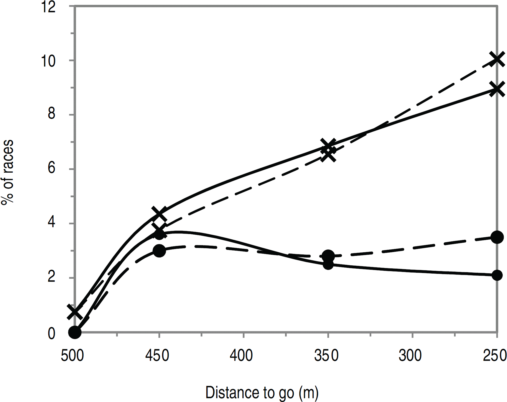
4.4 Summary of tactical implications

The key actions and race states that appear to influence race outcome, at each stage, are discussed here. The relative flying speed (FF) is the most important covariate. However, all models indicate that the faster rider will not always win and that tactics (quantified through the revealed covariates) have important effects. The importance of race tactics is demonstrated and compared for both the sequential and measurement error models in Figure 4 which shows the percentage of race outcomes correctly predicted over and above that predicted by assuming the faster rider wins (71%). This gives the proportion of races for which race states and actions applied before the end of each stage are influential. This is similar for both models, only 1% at 500 m to go rising to 9% at 250 m to go for the sequential model and slightly lower (8%) at 250 m to go for the measurement error model. Figure 4 also shows the proportion of races which can be accounted for by the actions and states applied during each stage (the percentage of race outcomes correctly predicted over and above that predicted by assuming that the faster rider wins at the current stage minus that at the previous stage), which remains approximately constant between 450 m and 250 m to go at around 3% for both models. Overall, the similar performance is not surprising considering that for the majority of races, the predicted win probabilities are similar for the two approaches.

Figure 4:

Percentage of races accounted for by race states and actions: (–x–) applied up to and including the end of the current race stage, (– $•$ –) during the current stage for the sequential (–––) and sequential measurement error models (– –).

As discussed in the previous section, the parameter estimates for both models are similar and so are the key actions and race states that appear to influence race outcome. From the parameters estimates which are displayed in Tables 2 and 3, the key actions and race states that appear to influence race outcome are identified for each stage.

In stage 1, a key finding is that the faster rider should increase track position between mark 1 and mark 2 and then either stay in the same track position or move to a lower one by the end of stage 1. He/she should also reduce the distance ahead over the stage if leading to better judge any sudden overtaking attempts or save energy for later in the race. A faster rider who is following should reduce the distance behind if following.

In stage 2, the slower rider can take advantage, if the opponent is not accelerating, by being behind and either in the same track position or lower than the faster rider by the end of the stage. The slower rider should also change track position between marks 1 and 2 in stage 2. Changing track position may allow the rider to save energy where the track gradient is high.

In stage 3, the faster rider has a very low chance of winning if he/she increases track position between mark 2 and the end of stage 3 when the opponent does not increase track position. This implies the faster rider has wasted energy by increasing track position and, hence, loses an advantage at later stages in the race.

In stage 4, both riders should overtake if behind; the faster rider should also be far ahead (2 m). It is better to overtake than undertake or already be leading the race at the beginning of this stage. A faster rider who is behind and does not over take or under take considerably reduces his/her chances of winning by decreasing track position during this stage (see Table 2; FLD(4) = 1), as the rider may have been unsuccessful in overtaking during this stage, and so overtaking during the remainder of the race will be more difficult to achieve.

5 Discussion and conclusion

A new approach is presented for analyzing the relationship between the outcome of a process with several stages and covariates that are revealed at each stage when the number of influential covariates is large. The approach extends the sequential model of Elisheva et al. (2000) by accounting for the measurement error in the estimated score. The approach is applied to the sprint event in track cycling with the aim of explaining race outcome and the following is found:

The score allows stable models to be created while capturing information from previous stages. Fewer terms in a sequential approach (in comparison to the naïve approach) also mean that the models are easier to interpret.

However, the score is measured with an error. A new approach is developed to incorporate for this error and we show for our application that not accounting for measurement error in the score leads to the estimated effect of the score being biased. For other terms, the bias is small, except for terms where the corresponding states or actions occurred infrequently in the dataset. The sequential model places more importance on race actions and less on the ratio of flying speeds (the covariate that dominates the score) than the sequential measurement error model.

In application to the sprint cycle race, the difference in predicted win probabilities between the sequential and measurement error models is also found, and it generally increases with each stage. The sequential model would predict on an average the more extreme probability, which when used in the subsequent stage via conversion to a score leads to an even more extreme probability. For some races, the probabilities predicted by the sequential model are unrealistically high or low, which are compounded at later stages. The sequential model predicts high chances of outcomes at 450 and 350 m to go for some races, but for this event it is highly unlikely that the outcome of the race has been decided at this stage. This illustrates that the measurement errors propagate through the stages in a sequential approach.

The measurement error technique adjusts the win probabilities (compared to the sequential approach) depending on the magnitude of the measurement error. The measurement error model predicts more extreme win probabilities when the measurement error variance is low and less extreme win probabilities when the measurement error variance is high. At stages 3 and 4, this effect also depends on the difference between the sequential and estimated scores, with the measurement error model predicting more extreme probabilities if the estimated score is more extreme and vice versa.

It is assumed that the true score is not correlated with the other observed covariates revealed in the current stage. This assumption is tested and shown to be valid for the application we described in Section 4. However, this may not be the case for a different application. Future work could involve adjusting the model to allow for such correlations. The approach could also be readily extended to incorporate variable selection techniques when little prior information is available about which covariates are influential on outcome.

Overall, we would suggest that it is essential to use measurement error techniques in a sequential approach to avoid bias in the estimation of the parameter for the score and, hence, to avoid misleading conclusions being drawn when determining the effects of covariates on outcome, especially when considering the relative importance of previous and current actions and states. These conclusions are applicable to the statistical analysis of sequential processes more generally outside of the sports example presented in this article, including, for example, medical intervention where extreme predicted probabilities could lead to the wrong decision being made about the most appropriate treatment. The real benefit of this approach will vary with application and may be assessed by preforming simulations.

Footnotes

Acknowledgments

This work has been supported by the Engineering and Physical Sciences Research Council of the UK under grant number EP/F005792/1. Data underlying the findings are fully available without restriction from [DOI: 10.17866/rd.salford.3839703]. We are grateful for the cooperation of the English Institute for Sport for use of the data and the help of Paul Barrett, Mike Hughes, and Duncan Locke and Jan Van Eijden of British Cycling.

References

Austin

(2008) Bootstrap model selection had similar performance for selecting authentic and noise variables compared to backward variable elimination: A simulation study Journal of Clinical Epidemiology , 61, 1009–1017.

Carroll

Ruppert

Stefanski

Crainiceanu

(2006) Measurement Error in Nonlinear Models: A Modern Perspective, 2nd edition . Boca Raton, FL: CRC Press.

Collett

(2002) Modelling Binary Data, 2nd edition . Boca Raton, FL: CRC Press.

Dobson

Barnett

(2008) An Introduction to Generalized Linear Models, 3rd edition . Boca Raton, FL: CRC Press.

Efron

(1983) Estimating the error rate of a prediction rule: Improvement on cross-validation. Journal of the American Statistical Association , 78, 316–331.

Efron

Tibshirani

(1993) An Introduction to the Bootstrap . New York and London: CRC Press.

Elisheva

Noya

Yana

Z-G

Dalit

Benjamin

(2000) Sequential logistic models for 30 days mortality after CABG: Pre-operative, intra-operative and post-operative experience—The Israeli CABG study (ISCAB). European Journal of Epidemiology , 16, 543–555.

Guo

Little

(2011) Regression analysis with covariates that have heteroscedastic measurement error. Statistics in Medicine , 30, 2278–2294.

Higdon

Schafer

(2001) Maximum likelihood computations for regression with measurement error. Computational Statistics & Data Analysis , 35, 283–299.

10.

Hildebrand

(1974) Introduction to Numerical Analysis, 2nd edition. New York and London: McGraw-Hill.

11.

Hill

van Wermeskerken

Lardenoye

J-WH

Phillips-Bute

Smith

Reves

Newman

(2000) Intraoperative physiologic variables and outcome in cardiac surgery: Part i. In-hospital mortality. The Annals of Thoracic Surgery , 69, 1070–1075.

12.

MATLAB (2007). The MathWorks Inc., Natick, Massachusetts.

13.

McCullagh

Nelder

(1989) Generalized Linear Models, 2nd edition. Boca Raton, FL: CRC Press.

14.

Moffatt

(2012) Sequential regression techniques with application to the individual sprint in track cycling. PhD thesis, Salford Business School, University of Salford, Salford, UK.

15.

Moffatt

Scarf

McHale

Passfield

Kui

(2014) To lead or not to lead: Analysis of the sprint in track cycling. Journal of Quantitative Analysis in Sports , 10, 161–172.

16.

Peduzzi

Concato

Kemper

Holford

Feinstein

(1996) A simulation study of the number of events per variable in logistic regression analysis. Journal of Clinical Epidemiology , 49, 1373–1379.

17.

R Development Core Team (2016) R: A Language and Environment for Statistical Computing . Vienna, Austria: R Foundation for Statistical Computing. URL http://www.R-project.org. (Accessed on 21 June 2016).

18.

Rabe-Hesketh

Pickles

Skrondal

(2003) Correcting for covariate measurement error in logistic regression using nonparametric maximum likelihood estimation. Statistical Modelling , 3, 215–232.

19.

Rosner

Spiegelman

Willett

(1990) Correction of logistic regression relative risk estimates and confidence intervals for measurement error: The case of multiple covariates measured with error. American Journal of Epidemiology , 132, 734–745.

20.

Sauerbrei

Schumacher

(1992) A bootstrap resampling procedure for model building: Application to the cox regression model. Statistics in Medicine , 11, 2093–2109.

21.

Seber

Lee

(2012) Linear Regression Analysis . New Jersey: John Wiley & Sons.

22.

Thoresen

Laake

(2000) A simulation study of measurement error correction methods in logistic regression. Biometrics , 56, 868–872.

23.

Tissot Timing (2016) Track cycling results. URL http://www.tissottiming.com/

24.

UCI (2016) Track cycling information. URL http://www.uci.ch/

25.

Van Wermeskerken

Lardenoye

J-WH

Hill

Grocott

Phillips-Bute

Smith

Reves

Newman

(2000) Intraoperative physiologic variables and outcome in cardiac surgery: Part ii. Neurologic outcome. The Annals of Thoracic Surgery, 69, 1077–1083.

26.

Vittinghoff

McCulloch

(2007) Relaxing the rule of ten events per variable in logistic and cox regression. American Journal of Epidemiology , 165, 710–718.

27.

Welsby

Bennett-Guerrero

Atwell

White

Newman

Smith

Mythen

(2002) The association of complication type with mortality and prolonged stay after cardiac surgery with cardiopulmonary bypass. Anesthesia & Analgesia , 94, 1072–1078.

Sequential regression measurement error models with application

Abstract

Keywords

1 Introduction

2 Review of the statistical analysis of sequential processes

3 Sequential regression models

3.1 Naïve sequential regression

3.2 Sequential regression

3.3 Sequential measurement error regression

3.3.1 Derivation of the sequential measurement error regression

4.1 Factors in the match sprint: Description and data collection

Table 1 :

Number of races, average flying speed in km/hr and the percentage of faster riders (by flying speed) who won the race for the dataset used to build the models by gender

4.3 Results

Table 2:

Parameter estimates, standard errors and p-values for the three models at stages 1, 2 and 3: 1, naïve sequential logistic regression; 2, sequential logistic regression; 3, sequential logistic measurement error regression.

Parameter estimates, standard errors and p-values for three models at stage 4: 1, naïve sequential logistic regression; 2, sequential logistic regression; 3, sequential logistic measurement error regression.

Definition of model covariates

Number of races by the absolute difference in win probabilities for the faster rider at 450 m, 350 m and 250 m to go as predicted by the sequential and measurement error models.

The average difference between the probabilities predicted by the sequential (Model 2) and sequential measurement error (Model 3) models (sequential minus measurement error) by the estimated score and measurement error variance

The association between observed and predicted responses at each stage for the sequential model (– • –) and the measurement error model (–x–) as measured by Somers’ D (adjusted using Efron's 0.682 estimator).

Figure 4:

Percentage of races accounted for by race states and actions: (–x–) applied up to and including the end of the current race stage, (– • –) during the current stage for the sequential (–––) and sequential measurement error models (– –).

Footnotes

Acknowledgments

References

The association between observed and predicted responses at each stage for the sequential model (– $•$ –) and the measurement error model (–x–) as measured by Somers’ D (adjusted using Efron's 0.682 estimator).

Percentage of races accounted for by race states and actions: (–x–) applied up to and including the end of the current race stage, (– $•$ –) during the current stage for the sequential (–––) and sequential measurement error models (– –).