Dipole and quadrupole resonance excitation in linear quadrupoles

Abstract

In the development of commercial quadrupole mass spectrometers, there is an interest in improving the performance characteristics such as transmission, resolution, and mass range. In particular, parametric and dipolar resonance excitation of trapping ions are used for linear quadrupole mass filters. Theoretical methods and numerical simulation of ion trajectories were applied for study of ion-optical properties. The review is devoted to description of different excitation methods to improve QMF performance and consists of three parts. The first part presents the results of a linear ion trap simulation for various operating conditions and excitation methods. The second part considers the effects of dipole excitation (DE) on the performance of the quadrupole mass filter. The last part analyzes the formation of stability islands by different methods of quadrupole excitation. To date conditions of mass separation in quadrupole mass filters with sin wave supply were described for stability islands of the first and third stability regions formed by quadrupole and DE. By complicating the electronics such methods allow to overcome the destructive influence of electric field distortions and obtain a resolving power and ion transmission efficiency comparable with commercial devices. At quadrupole resonance excitation by a two-frequency signal, it is possible to reduce the length of electrodes three times without losses in resolution and transmission, which reduces the cost of rod set production with micrometer accuracy. Dipole resonance excitation allows controlling the shape of the mass peak by changing amplitude and phase of the auxiliary AC signal. The main factors affecting the resolving power of a linear ion trap are described theoretically. The numerical modeling results are confirmed by experiment.

Introduction

Scientists have long sought alternatives to magnetic isotope separation. W. Paul in 1953 proposed to use quadrupole quasi-static electromagnetic fields for this purpose. ¹ The theoretical basis of ion separation is the properties of the Mathieu equation that describes the ion motion in quadrupole RF fields with a sinusoidal power supply. ² Operation quadrupole mass spectrometer requires a high precision of machining and assembling of rods with high accuracy, and a development of very stable and controllable power supplies. ³

Various quadrupole mass filters are used as quadrupole analyzers, linear ion traps and ion guides because of their analytical capabilities, compact sizes and relatively low price. A modern presentation of quadrupole mass spectrometry basics can be found in books.^4,5

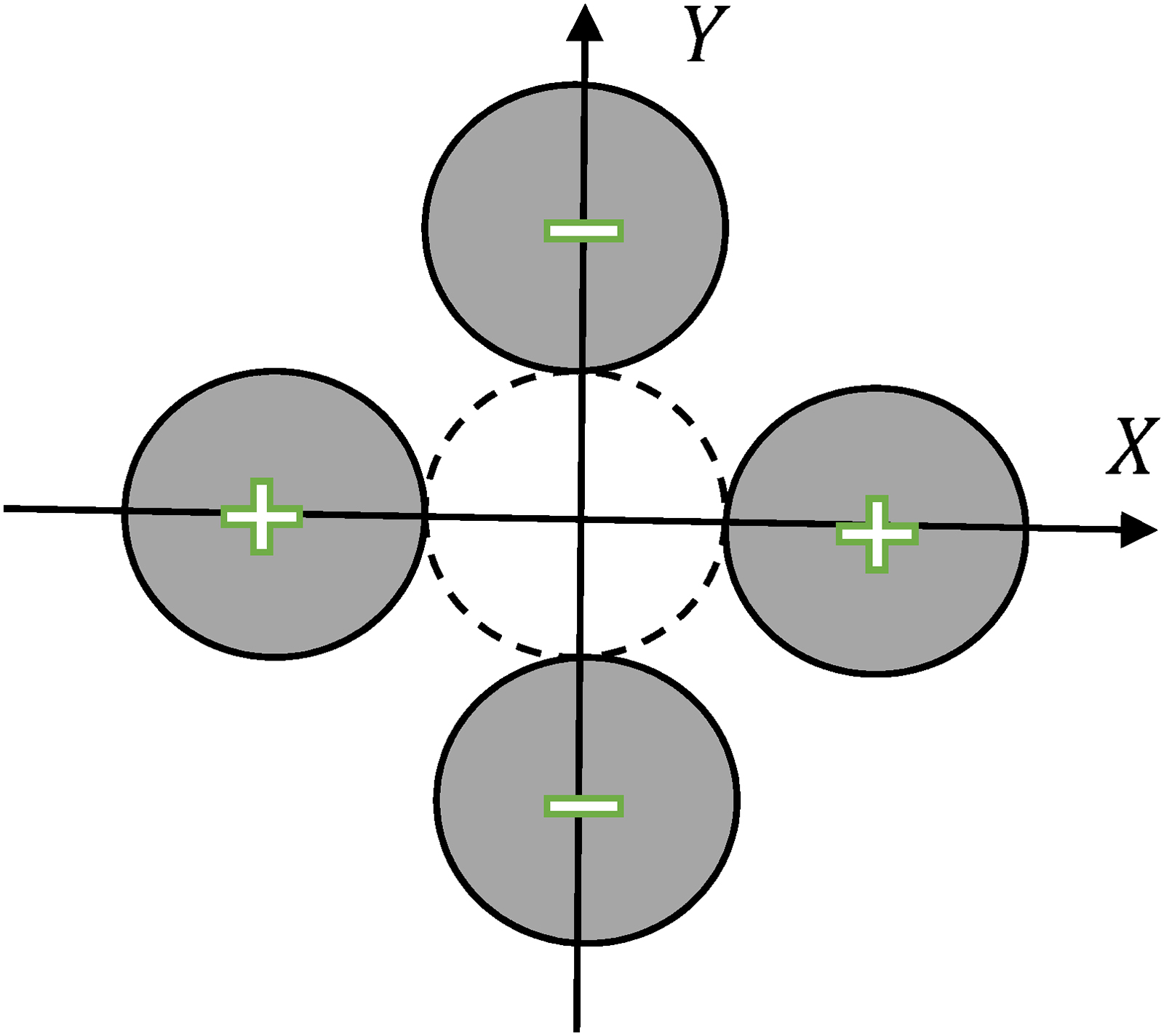
The ion oscillations in RF ideal quadrupole electric fields have a discrete spectrum, which is defined by the point $(a,q)$ on the mass filter stability diagram. The oscillations of ions are independent of the transverse x and y coordinates of the analyzer. The frequencies of this spectrum are characterized by the stability parameters (characteristic exponents) ${\beta }_x$ and ${\beta }_y$ . Dipole excitation (DE) is created by the difference of potentials applied to pairs of X or Y electrodes. X rods have positive potential $+U$ and Y rods have negative potential $\text{–}U$ for filtration of positive ions (Figure 1). Figure 1 shows the structure of the QMF electrodes, which are supplied with a voltage of $\pm (U+Vcos\mathrm{\Omega }t)$ .

Figure 1.

X and Y directions and sign polarity of rods for the DC potential.

When the AC frequency of the dipole potential and one of the frequencies of the ion's natural oscillations are equal, a resonance occurs when the ion unlimitedly increases the oscillation amplitude. When an additional quadrupole AC of small amplitude is applied, a parametric resonance occurs, leading to the formation of stability islands on the $(a,q)$ diagram. In this paper, resonance excitation effects are discussed to improve the performance of linear quadrupoles with sin wave supply and harmonic auxiliary excitation. The physical side of the processes of parametric and DE of ion oscillations by different methods such as frequency and amplitude modulation is emphasized. The aim of the paper is to describe the above processes on the basis of analytical description and numerical modeling of ion motion in linear and nonlinear quadrupole fields.

P. Reilly group from Washington State University obtained important results for ion trap, ion guides, and QMF with driving rectangular waveforms.^6–8 The concept of a digitally driven mass filter has been moved from a theoretical concept to reality. ⁷ The mass spectrum of lysozyme (m/z ∼ 2000) with low impulse amplitude about 300 Volts was obtained. The use of two rectangular frequency-asymmetric and amplitude-asymmetric waveforms of potentials leads to splitting of the first region A into stability islands. ⁸ The ratio of the amplitudes of the two applied rectangular potentials controls the width of the instability bands.

A leading group of scientists from Purdue University presented an excellent review on linear and nonlinear resonances in quadrupole ion traps. ⁹ The effect of higher order fields on ion excitation and mass analysis is described. The ion trap resonance methods such as isolation, activation, ejection and mass-selective detection, charge detection are presented. A formula for the resolution of LIT as a function of pressure and ion motion relaxation time caused by collisions with the bath gas molecules is given.

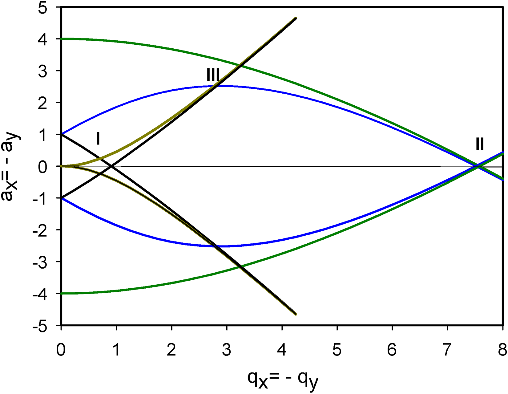
We discuss the separation modes with resonant excitation in the first (I), second (II), and third (III) stability regions of the Mathieu equation following the notations of the review paper. ¹⁰ The mass filter stability diagram for the three stability regions is shown in Figure 2.

Figure 2.

Stability diagram for the Mathieu equation with specified regions I, II and III.

We do not take into account the input fringing fields because they practically do not affect the dipole and quadrupole excitation processes for a linear ion trap since the regions with fringing fields (which have dimensions of about $1.5r_0$ ) are small compared to the rods’ length. The resolution of the mass filter under resonant excitation is also affected by the quality of the quadrupole field, determined by micron errors in electrode fabrication and assembly. A comparison of the transmission and resolution of a QMF with an ideal field and the field produced by circular rods is given. For this purpose, the field of circular electrodes is described by a complex potential. ¹¹ The problem of input fringing fields is solved by means of a Brubaker prefilter (delayed DC ramp), ¹² by using electrodynamic ion funnels ¹³ or by gas damping in quadrupole or hexapole RF fields. ¹⁴

Modeling linear ion traps

Fisher first described the process of dipole resonance excitation of ion oscillations in a 3D ion trap in 1959. ¹⁵ Dipole resonance excitation of ion oscillations has found application for mass-selective excitation and ion ejection of 3D Paul traps,^16,17 for axial^18,19 and radial ²⁰ ion ejection in linear quadrupole linear traps. Here we will discuss modeling of the ion linear ion trap operation with dipole and quadrupole excitation. Theoretical and experimental aspects of this topic are considered in references.^21–31

Ion motion equations

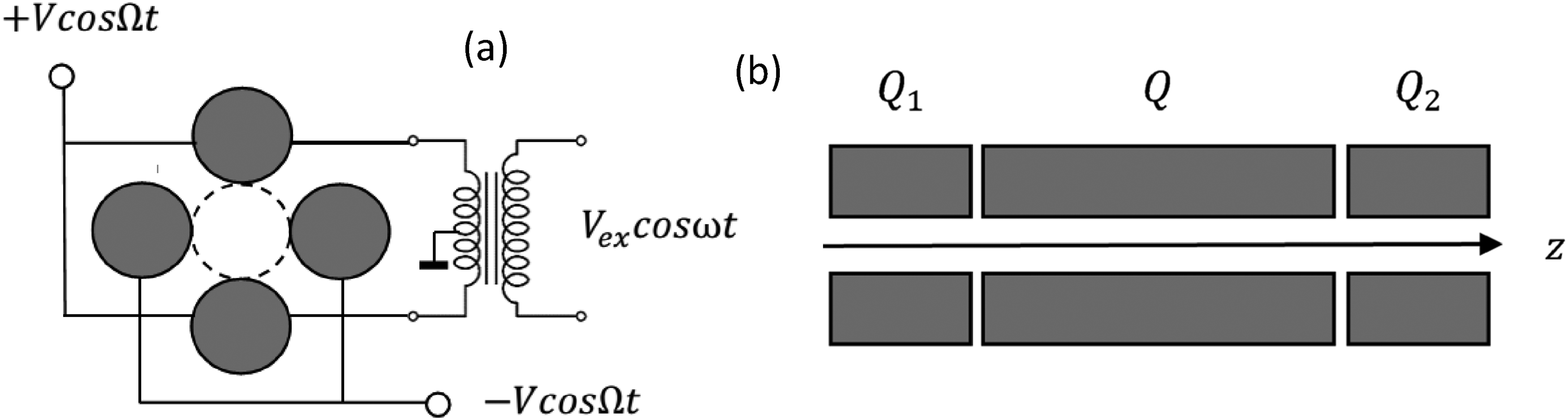
We denote one pair of opposite quadrupole rods as X rods and the other pair as Y rods. The term DE is used because an additional alternating voltage $V_{ex}cos(\omega t+\alpha )$ is applied to a pair of opposite electrodes through a toroidal transformer^30,31 (Figure 3). These electrodes act as a flat capacitor, when the field strength is equal to $E=A_1{V}_{ex}/r_0$ , where $A_1$ is an amplitude of dipole component of the field expansion in series on spatial harmonics^11,32 for DC potential $(-1,1)$ on X rods and $(0,0)$ on Y rods.

Figure 3.

(a) Power scheme for the linear ion trap. The $\pm V\cos \mathrm{\Omega }t$ voltage is used to create the quadrupole field and the $V_{ex}$ cosωt voltage is used to create the resonant excitation of the ion oscillations. (b) Linear ion trap. Resonant dipole mass-selective detection is performed through a slot in the electrode in the central section.

External quadrupoles Q1 and Q2 are placed at the ends of the trap (Figure 3(b)). The analyzed ion beam is introduced through the Q1 quadrupole into the Q trap along the z-axis. In the x,y plane, the ions are trapped by the RF quadrupole electric field, which is created by the RF voltage applied to the four electrodes. The external quadrupoles Q1 and Q2 are also supplied with RF potential. In order to hold the ions along the z-axis after the trap Q is filled with ions, positive + U potentials of the order of 100 V are applied to the external quadrupoles in the analysis of positive ions. This locks the ions in the Q trap. Mass-selective ion ejection is carried out through the slot of one of the electrodes of the trap Q.

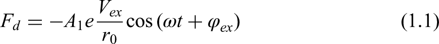
The force $F_d$ acting on the ion from the dipole field is^33,34

$$F_d=-A_{1}e{\displaystyle \frac{V_{ex}}{r_0}\cos (\omega t+{\phi }_{ex})}$$

(1.1)

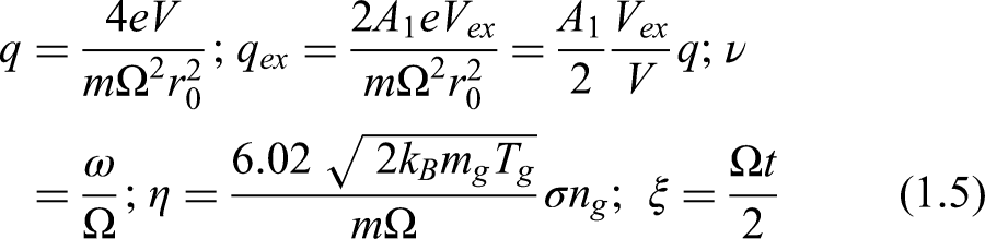
Where e is the ion charge, $r_0$ is the field radius, $\omega$ is the angle resonant frequency, and ${\phi }_{ex}$ is the phase shift.

The drag force $F_f$ on an ion from buffer gas^33,35 is

$$F_f=-{\displaystyle \frac{3.01\sqrt{2k_B{m}_g{T}_g}}{2}\sigma n_{g}v}$$

(1.2)

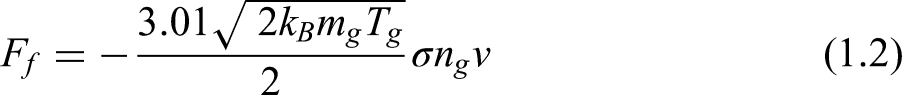
Where $k_B$ is Boltzmann's constant, $m_g$ is the collision gas mass, $\sigma$ is the collision cross-section of the ion, $n_g$ is the gas numberdensity, $T_g$ is the gas temperature, and v is the ion velocity.

Four parallel symmetrically arranged round rods produce an electric potential

$$\mathrm{\Phi }(x,y,t)=Re[\phi (z)]Vcos\mathrm{\Omega }t$$

(1.3)

Here $\phi (z)=A_2{z}^2+A_6{z}^6+A_{10}{z}^{10}+\dots$ is a complex potential, $z=x+iy$ is complex coordinate. The weighting factors $A_k$ of the field decomposition into sum of multipoles can be calculated by the methods outlined in papers.^11,32

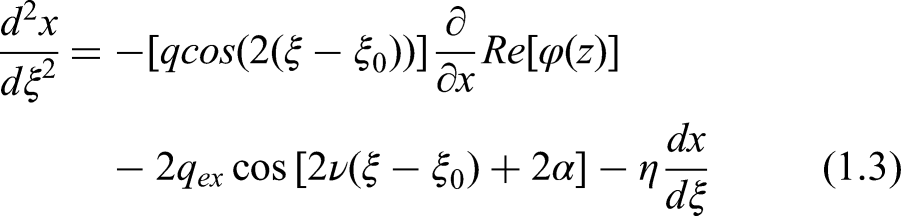
Taking into account these forces acting on the ion and using Newton's second law, we obtain the equations of ion motion in the round rods field:

$${\displaystyle \frac{d^{2}x}{d{\xi }^2}=-[qcos(2(\xi -{\xi }_0))]{\displaystyle \frac{\mathrm{\partial }}{\mathrm{\partial }x}Re[\phi (z)]-2q_{ex}\cos [2\nu (\xi -{\xi }_0)+2\alpha ]-\eta {\displaystyle \frac{dx}{d\xi }}}}$$

(1.3)

$${\displaystyle \frac{d^{2}y}{d{\xi }^2}=-[qcos(2(\xi -{\xi }_0))]{\displaystyle \frac{\mathrm{\partial }}{\mathrm{\partial }y}Re[\phi (z)]-\eta {\displaystyle \frac{dy}{d\xi }}}}$$

(1.4)

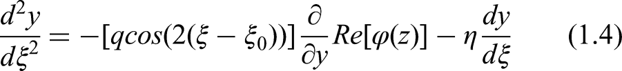
Equations (1.3) and (1.4) are presented in dimensionless variables, where the x and y coordinates are normalized to $r_0$ ,

$$q={\displaystyle \frac{4eV}{m{\mathrm{\Omega }}^2{r}_0^2};q_{ex}={\displaystyle \frac{2A_{1}e{V}_{ex}}{m{\mathrm{\Omega }}^2{r}_0^2}={\displaystyle \frac{A_1}{2}{\displaystyle \frac{V_{ex}}{V}q;\nu ={\displaystyle \frac{\omega }{\mathrm{\Omega }};\eta ={\displaystyle \frac{6.02\sqrt{2k_B{m}_g{T}_g}}{m\mathrm{\Omega }}\sigma n_g;\xi ={\displaystyle \frac{\mathrm{\Omega }t}{2}}}}}}}}$$

(1.5)

Resonant frequencies

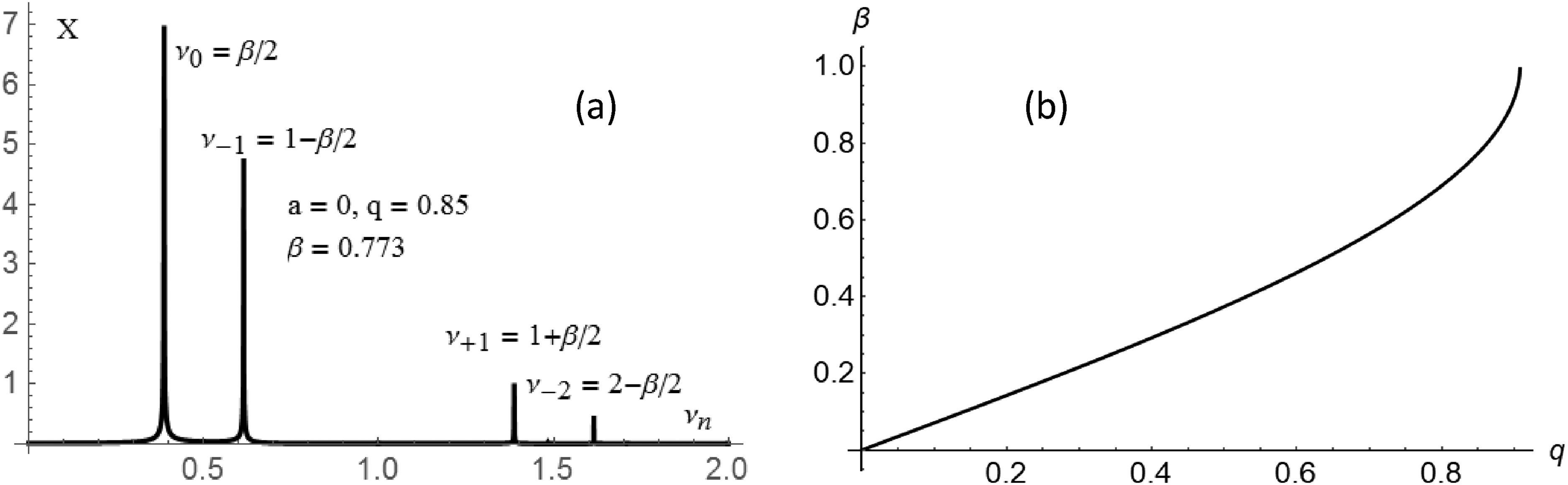
The discrete spectrum of ion oscillations is represented by a set of infinite number of temporal harmonics with frequencies ${\omega }_k=\frac{|2k+\beta |\mathrm{\Omega }}{2},k=0,\pm 1,\pm 2,\dots$ . ³⁶ Figure 4(a) shows the frequency spectrum for $q=0.85(\beta =0.77295)$ . The spectrum consists mainly of four temporal harmonics. The dependence of the parameter $\beta$ on the injection parameter q is shown in Figure 4. The dependence of $\beta$ on the injection parameter q is shown in Figure 4(b). The linearity region $\beta (q)$ approximately lies between $q\cong 0$ and 0.4. The value of $\beta =1$ is attained at $q=0.9080$ .

Figure 4.

(a) Frequency spectrum ${\nu }_k=\left|k+\frac{\beta }{2}\right|$ of ion oscillation at point $a=0,q=\mathrm{0.85.}$ (b) The dependence of the characteristic index $\beta$ on the parameter q of the Mathieu equation $\stackrel{\ddot{+}}{x}(2q\cos 2\xi )x=0$ in the first stability region.

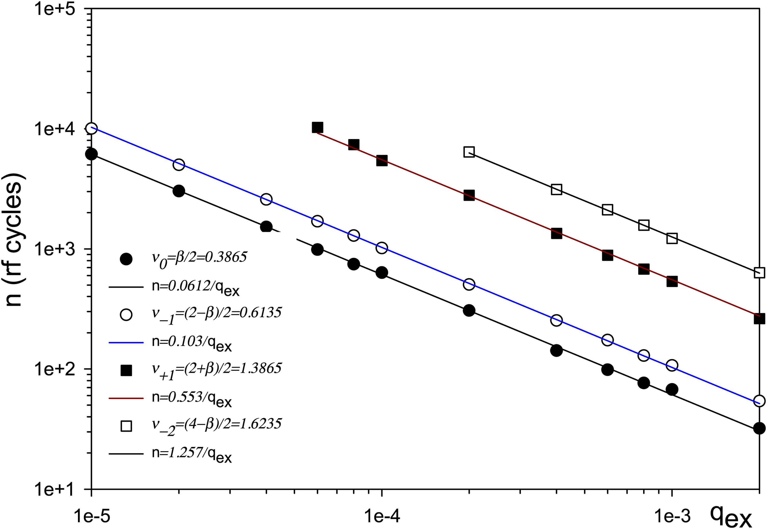
The amplitude X of the ion oscillations decreases rapidly with growth of the frequency ${\nu }_k$ . At a given value of the injection parameter $q=0.85$ four resonance frequencies ${\omega }_k=0.3685\mathrm{\Omega },0.6315\mathrm{\Omega },1.3685\mathrm{\Omega },1.6315\mathrm{\Omega }$ are possible. It is illustrated in Figure 5, where the dependence of the number of periods n of the RF field on the amplitude $q_{ex}$ of the dipole voltage for four values of the resonant frequencies ${\nu }_k=0,k=0,-1,k=1,k=-2$ . All values $n(q_{ex})$ are inversely proportional to $q_{ex}$ ; the smaller the harmonic amplitude (Figure 5), the higher the required values of n and $q_{ex}$ . Here n is the number of RF field periods for which the amplitude of the ion oscillations will be equal to $r_0$ .

Figure 5.

Dependence of the required excitation time n vs the excitation amplitude $q_{ex}.$ Initial conditions: $x_0=y_0=0.01r_0$ , $v_{x0}=v_{y0}=0.016\pi r_{0}f$ , ${\xi }_0=\alpha =0$ . ³³

The variation of the excitation time n, with $q_{ex}$ , at $q=0.85$ ( $\beta =0.77295$ ), is shown in Figure 5 for the four main harmonics with frequencies ${\nu }_0$ , ${\nu }_{-1}$ , ${\nu }_1$ , and ${\nu }_{-2}$ . The initial conditions are $x_0=y_0=0.01r_0$ , $v_{x0}=v_{y0}=0.016\pi r_{0}f$ . On a log–log scale, the dependence $n(q_{ex})$ give straight lines with a slope of $-1$ . Thus, the function $n(q_{ex})$ has a universal form $n=c/q_{ex}$ , where c is a constant which depends on the ejection parameter q ( $q_{ejec}$ ), the excitation frequency ${\nu }_k$ , and the initial conditions: the initial positions $x_0,y_0$ , velocities $v_{x0}=v_{y0}$ , initial rf phases ${\xi }_0$ , and the phase shift $\alpha$ between the rf voltage and the dipolar excitation.

Resolution of LIT

The resolving power of the mass-selective resonance excitation is controlled by two main factors: (i) the excitation time and the width of the excitation frequency spectrum of the ion ensemble and (ii) the standard deviation between the mass band and the width of the excitation spectrum. ³³ The width of the spectrum $\mathrm{\Delta }\omega$ of the ion ensemble is related to the finite excitation time $\theta$ as ³⁷

$$\mathrm{\Delta }\omega =2\pi /\theta$$

(1.6)

This means that the longer the wave train, the narrower the frequency spectrum of the excitation resonance signal. Here we express the excitation time $\theta$ in the number of RF field periods.

Consider the second important factor: the resolving power of resonant excitation is determined by the deviation between the excitation frequency band $\mathrm{\Delta }\nu$ and the ion mass band $\mathrm{\Delta }m$ :

$$\mathrm{\Delta }\nu /\mathrm{\Delta }m=q/2m\cdot d\beta /dq$$

(1.7)

The formula for the linear ion trap resolution power ³³

$$R={\displaystyle \frac{m}{\mathrm{\Delta }m}={\displaystyle \frac{1}{2}{\displaystyle \frac{d\beta }{dq}qn={\displaystyle \frac{1}{2}{\displaystyle \frac{d\beta }{dq}{\displaystyle \frac{qF}{V_m}}}}}}}$$

(1.8)

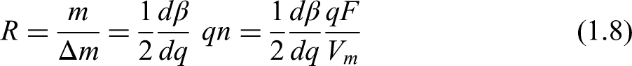
follows from equations (1.6) and (1.7), here $\frac{d\beta }{dq}$ is a derivative of the function $\beta (q)$ which is shown on Figure 4(b), $q=q_{ejec}$ is the ejection parameter, n is excitation time (in RF cycles), $F=2\pi /\mathrm{\Omega }$ is cycle frequency, and $V_m=\frac{1Th}{n}F$ is scan speed. Thus, the mass selectivity of resonant DE is directly proportional to the derivative $d\beta /dq,$ the injection parameter $q_{ejec}$ , and the RF field frequency F and inversely proportional to the scanning speed $V_m=F/n$ . These patterns are confirmed by experimental results. ¹⁹ There are other approaches to estimating LIT resolution.^16,17,23,24

Excitation contour

The mass selectivity of the dipolar excitation depends on the excitation time n. Ions with similar mass-to-charge ratios, excited for a finite time $\theta$ , have approximately the same oscillation spectra and will be detected at the same time. Due to this circumstance, it is feasible to introduce the excitation contour as a general characteristic of the mass selectivity excitation of trapped ions. ²¹ The share $S(q)$ of excited ions depends on the variation of the parameter $q$ (Eq. 1.5) at constant ion mass and amplitude $V$ of the scan: $S(q)=N_{ex}/N$ , where $N_{ex}$ is the number of ions trapped with parameter q for which $x(t)\ge r_0$ , $t\le n2\pi /\mathrm{\Omega }$ .

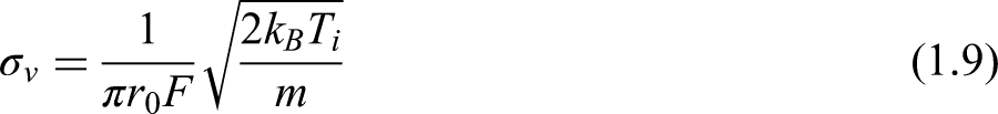
A numerical method of trajectories simulation is used to calculate the excitation contour. In the computation, the ion ensemble is characterized by a random distribution of initial coordinates and velocities. ³⁴ It is assumed that, as a result of precooling of the ions in the quadrupole with a buffer gas, the ions at the entrance to the trap obey the Gaussian distribution. Therefore, we assume that the initial coordinates and velocities have a Gaussian distribution with standard deviation ${\sigma }_x={\sigma }_y$ in the $x$ and y directions and standard deviation ${\sigma }_v$ of the transverse velocities. ³⁴ The standard deviation ${\sigma }_v$ is given by

$${\sigma }_v={\displaystyle \frac{1}{\pi r_{0}F}\sqrt{{\displaystyle \frac{2k_B{T}_i}{m}}}}$$

(1.9)

where $T_i$ is the ion temperature. Integration of equations (1.3) and (1.4) was carried out numerically. Initial data are random initial conditions, integration interval $[0,n\pi ]$ , excitation parameter $q_x$ , number of trajectories N and number $N_p$ of trajectories per point in the contour $S(q_i)$ , and initial and final values $q_a$ and $q_b$ . Each point on the curve $S(q)$ is obtained by computing N trajectories. The excitation frequency ν was fixed and $S(q)$ was calculated for values of q close to the corresponding excitation frequency. The program calculates the number of ion trajectories $N_{ex}$ , whose coordinates correspond to the condition $x\ge 1$ in the at a given point $q_i$ . The fraction of ions that reach the electrodes is $S(q_i)=N_{ex}/N_p$ . Usually 500 trajectories of ions at a point $q_i$ is enough for an adequate counting statistics. ³³

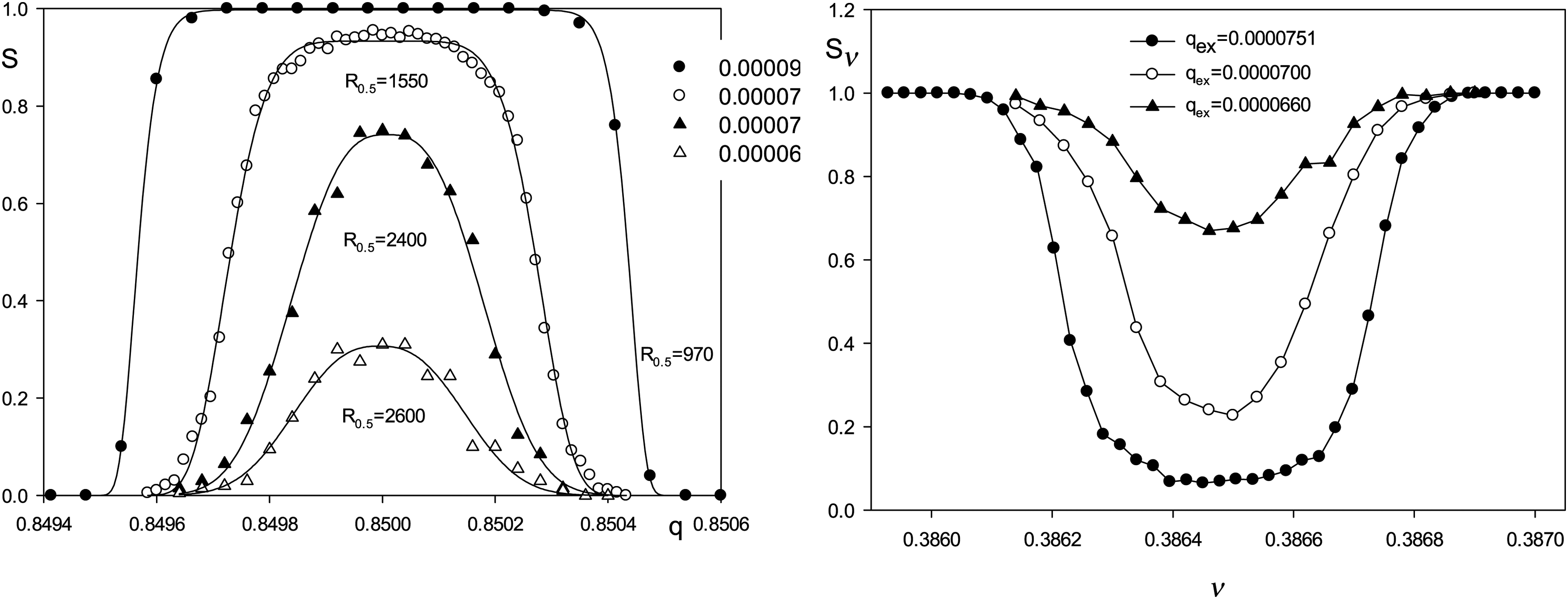
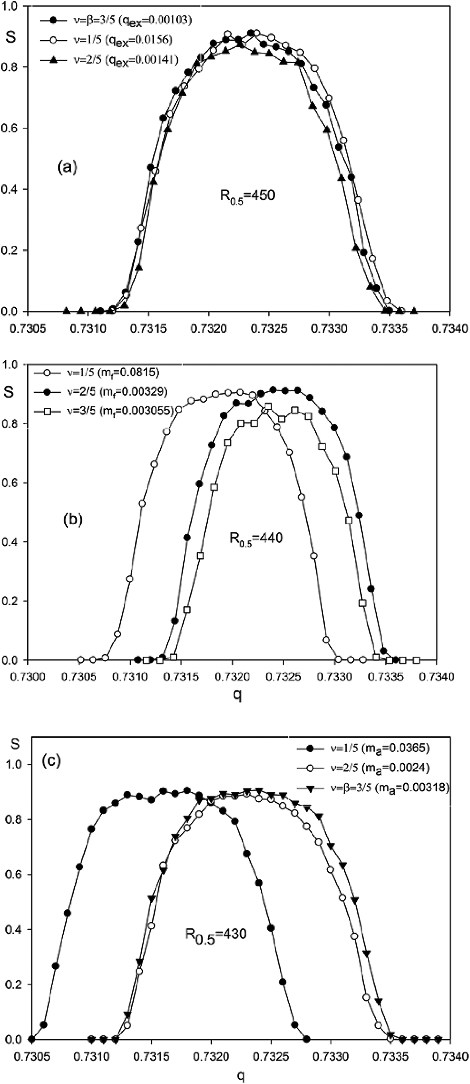
Figure 6(a) shows the excitation contours at different DE amplitudes $q_{ex}$ or $V_{ex}$ in Volts, respectively. As the amplitude $q_{ex}$ increases, the resolution decreases and the intensity S corresponding to the maximum peak increases. The contour with 100% excitation ( $S=1$ ) and maximum resolving power should be noted. Further, with the increase of $q_{ex}$ value, the contour width increases while the resolving power decreases. We can say that in this case there is an over excitation.

Figure 6.

(a) Contours $S(q)$ , with values of $q_{ex}$ of ●, $0.000092$ ;○, $0.000076$ ; ▴, $0.000070$ and Δ, $0.000066$ , corresponding to $V_{ex}=0.250,0.207,0.190$ and $0.179V$ , respectively. (b) Frequency response curves $\mathrm{\Sigma }(\nu )$ for $q_{ejec}=0.85$ with $q_{ex}=0.0000751$ , $0.0000700$ and $0.0000660;$ here $n=1000$ . ³³

Frequency response curves ${\mathrm{\Sigma }}_{\nu }$ obtained by changing the frequency $\nu$ at a constant value of $q=0.85$ are shown in Figure 6(b) for values of $q_x$ =0.0000751, 0.0000700, and 0.0000660 ( $n$  = 1000). The excitation conditions are the same as in Figure 6(a). The frequency resolution $R_{0.5}=\nu /\mathrm{\Delta }\nu$ at one half the peak depth decreases with increasing $q_{ex}$ . Note that ${\mathrm{\Sigma }}_{\nu }\ne 1-S(q)$ because the functions ${\mathrm{\Sigma }}_{\nu }$ and $S(q)$ have different arguments, $\nu$ and q. This excitation pattern is observed experimentally. ¹⁹

Effects of gas damping

The motion of ions in a rarefied buffer gas, when the mass of the gas molecule is much smaller than the mass of the ion, was simulated with the drag force (1.2), which is proportional to the ion velocity. ³³

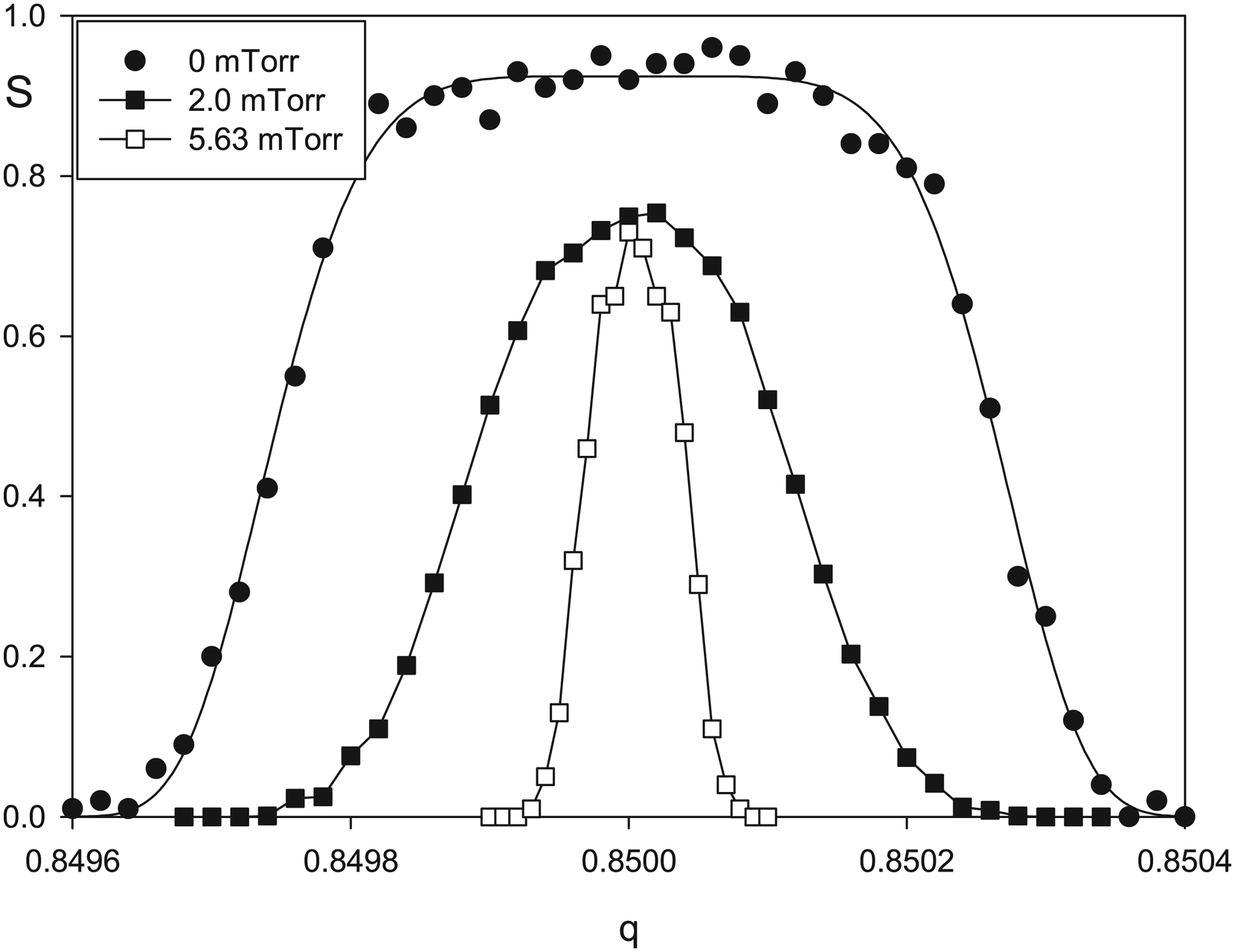
Protonated reserpine ions ( $m=609$ , with collision cross-section of $280{\text{Å}}^2$ ³⁸ ) and a $N_2$ buffer gas with pressures $1\text{–}3$ mTorr were modeled. Adding a buffer gas to the traps is necessary for cooling and concentrating the ions in the near-axis region of the linear trap. As a result, the presence of buffer gas leads to an increase in mass-selective ejection and resolution power. This gas damping effect is illustrated in Figure 7.

Figure 7.

Excitation contours $S(q)$ at a buffer gas pressure of $2.815$ mTorr for excitation times of 1000 and 2000 rf cycles. Resonant frequency ${\nu }_{-1}=(2-\beta )/2.$ Dipolar amplitudes $q_{ex}=0.00049971$ and $q_{ex}=0.0005069$ , $m=609$ Th, $q_{ejec}=0.85$ . ³³

Figure 7 shows two peaks $S(q)$ with high resolution $R_{0.5}=10500$ and $31480$ . At the RF field frequency $F=1$ MHz, the scan rates are $1000$ Th/s and $2000$ Th/s, respectively. Doubling the excitation time n approximately triples the resolution $R_{0.5}$ . Achieving $30,000$ resolution requires high stability and reproducibility of the dipole potential with an error of about $0.02\text{\%}$ . A change of q only $0.00002$ leads to $S=1$ or $S=0$ .

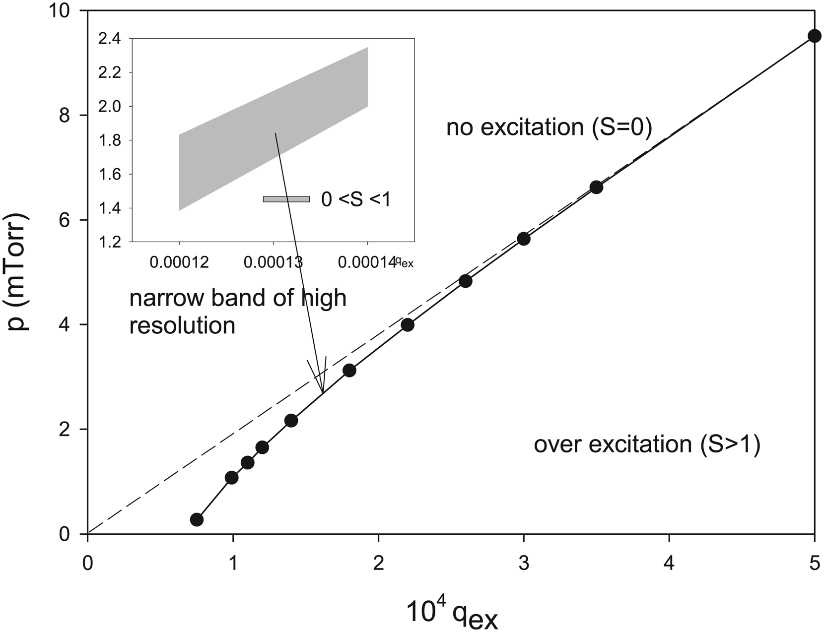
Figure 8 shows the dependence of the excitation band position on the parameter plane: the dipole potential amplitude $q_{ex}$ and the buffer gas pressure p. The value of $q_{ex}$ in the graph is determined from the condition $S(q_{ex})=1/2$ , i.e. at which the excitation efficiency is $50\text{\%}$ . The value $S=1$ corresponds to the peak height (Figure 6(a)). The part of this band where $0<S<1$ is shown in detail in the upper figure. The band of the $q_{ex}$ and p parameters narrows as the pressure p increases and asymptotically degenerates into a straight line p [mTorr] =  $9510$ $q_{ex}$ . This straight line divides the $q_{ex},p$ plane into two regions, $S=0$ (no excitation) and $S=1$ (over excitation). Over excitation means that at a fixed pressure p, increasing the amplitude $q_{ex}$ of the dipole AC potential leads to a broadening of the peak at $100\text{\%}$ excitation.

Figure 8.

The relation between the buffer gas ( $N_2$ ) pressure and $q_{ex}$ determined with $S(q_{ex})$ $\approx$ $1/2$ . The dashed line is the asymptotic line p [mTorr] =  $9510\times q_{ex}$ . ${\sigma }_x=0.01r_0$ , $T_g$  =  $1000$ K, $q_{ejec}=0.85$ , $\nu =\frac{\beta }{2},n=1000$ . ³³

The concept of modeling dipole mass-selective ion ejection in terms of the excitation contour reflects the basic patterns of the resonant excitation process of ion oscillations. The two excitation frequencies ${\nu }_0$ and ${\nu }_{-1}$ give approximately the same resolution because oscillation spectra amplitudes are approximately equal (Figure 4(a)). Excitation time n and amplitude $q_{ex}$ are strongly coupled as $q_{ex}\sim 1/n$ or $V_{ex}\sim F/V_m$ . With gas damping the resolution is up by factor of 6 (e.g. from $1,625$ to $10,000$ in Figure 7).

The presented results are in qualitative agreement with experimental observations for both radial and axial ejection from linear traps. So at low scan speeds the dipolar voltage should be small and the resolution is highest,^16–18 the resolution is greater with excitation at $q=0.85$ than at lower $q$ ^4,5,16,20 and a low pressure buffer gas can increase the mass resolution.^10,23

Resonance excitation profiles with a mass resolution of >21 500 with a low trap pressure (3.8 ${10}^{-5}$ Torr), low excitation amplitude (3 mV), long excitation period (100 ms), and a high Mathieu $q=0.8$ value was obtained. ³⁹ One must note that for a precise description of the mass peak shape, it is necessary to take into account the three-dimensional field near the slit of the electrode through which ions are ejected to the detector. Besides there is the three-dimensional fields near the detector. The ion filling of the trap is also determined by the LIT acceptance, which is influenced by the input three-dimensional fringing field, as well as distortions of the analyzer's field. Nevertheless, resonance excitation profiles of ³⁹ qualitatively confirm the results of trajectory modeling: high resolution is achieved at low excitation amplitude ( $q_{ex}$ ), long excitation time ( $n$ ) and high value of the Mathieu parameter $q$ in the presence of buffer gas.

LIT with impulse power supply

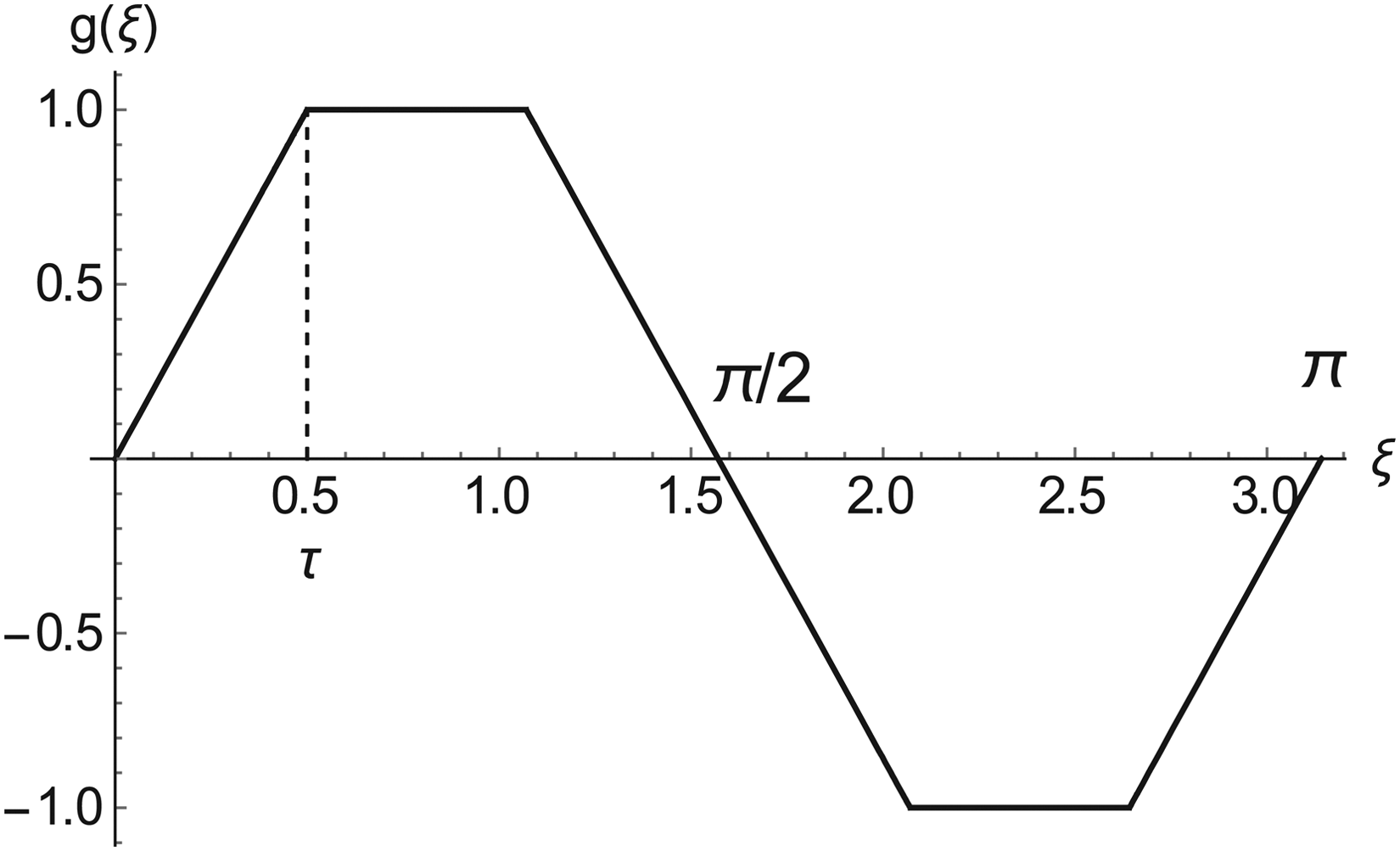
A simulation of the LIT with impulse power supply and sinusoidal DE is presented in detail in. ⁴⁰ Consider the trapezoidal shape of the quadrupole RF voltage for the linear ion trap shown in Figure 9. The impulse shape is described by a single parameter $\tau$ . For $\tau =0$ , the impulse shape is rectangular. The ion motion equation in an ideal quadrupole field with impulse power supply is

$$x{}^{\mathrm{″}}(\xi )+2qg(\xi )x(\xi )=0$$

(1.10)

where x is the normalized coordinate to $r_0$ , $\xi =\mathrm{\Omega }t/2$ is dimensionless time, and g(ξ) is a periodic function of time (Figure 9),

$$q={\displaystyle \frac{4eV}{m{\mathrm{\Omega }}^2{r}_0^2},\mathrm{\Omega }={\displaystyle \frac{2\pi }{T}}}$$

(1.11)

Figure 9.

Trapezoidal pulse signal with period $\pi$ and $\tau =\pi /8$ .

$V$ is pulse amplitude, m and e are ion mass and charge, T is pulse signal period.

Let us establish the relationship between the parameters $q$ and $\beta$ . First we will determine the transformation matrix M of initial coordinates $x_0$ and velocities ${\dot{x}}_0$ trough period $\pi$ . ³⁸ For finding matrix M is required to solve the equation with initial conditions $x_0(0)=1,\dot{x}(0)=1$ and $x_0(0)=0,\dot{x}(0)=1$ . To solve this problem, one can use, for example, the matrix method. ⁴¹ For the rectangular form of pulses, the matrix M has an explicit form

$$M=\left[\begin{array}{cc}\cos Q\cosh Q-\sin Q\sinh Q& \sqrt{2q}(\cos QsinhQ-\cosh QQ\sin Q\\ (\cosh Q\sin Q+\cos QQ\sinh Q)/\sqrt{2q}& \cosh Q\cosh Q+\sin Q\sinh Q\end{array}\right]$$

(1.12)

where $Q=\pi \sqrt{q/2}$ . This follows from the fact that at the positive top of the pulse, equation (1.10) is expressed via the Cos function and the negative bottom via Cosh. The trace of the matrix M determining the parameter $\beta$ is

$$\beta =\mathrm{co}{\mathrm{s}}^{-1}(\cos Q\cosh Q)/\pi$$

(1.13)

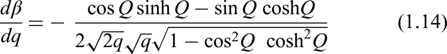
The derivative $d\beta /dq$ , which determines the standard deviation between the ion mass and the excitation frequency $\omega =\beta \mathrm{\Omega }/2$ , is

$${\displaystyle \frac{d\beta }{dq}=-{\displaystyle \frac{\cos Q\sinh Q-\sin Q\cosh Q}{2\sqrt{2q}\sqrt{q}\sqrt{1-\mathrm{co}{\mathrm{s}}^{2}Q\cos {\mathrm{h}}^{2}Q}}}}$$

(1.14)

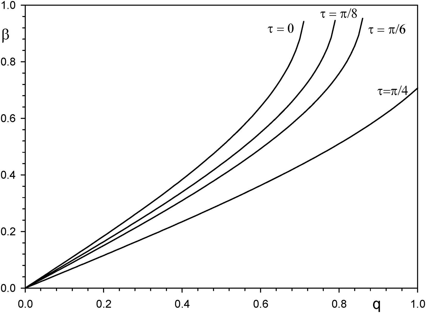
Note that $\beta (q=0.5)=0.5$ and at the stability boundary $q(\beta =1)=0.712493$ … for the first region. The curves $\beta (q)$ are shown in Figure 1.8 for the shape of pulses with the parameters $\tau =0,\pi /8,\pi /6$ , and $\pi /4$ . When changing the impulse shape from rectangular ( $\tau =0$ ) to triangular ( $\tau =\pi /4$ ), the value of $\beta$ decreases at a given value of q. At the same time, the stability boundary q (for $\beta =1$ ) along the q -axis increases.

Ion motion in RF quadrupole fields is determined by the same equations (1.3, 1.4) as for sinusoidal RF voltage changing $\cos 2(\xi -{\xi }_0)$ on general function $g(\xi -{\xi }_0)$ :

$${\displaystyle \frac{d^{2}x}{d{\xi }^2}+2q\cdot g(\xi -{\xi }_0){\displaystyle \frac{\mathrm{\partial }}{\mathrm{\partial }x}Re[\phi (z)]+2q_{ex}\cos (\beta \xi +\alpha )=0}}$$

(1.15)

$${\displaystyle \frac{d^{2}y}{d{\xi }^2}+2q\cdot g(\xi -{\xi }_0){\displaystyle \frac{\mathrm{\partial }}{\mathrm{\partial }y}Re[\phi (z)]=0}}$$

(1.16)

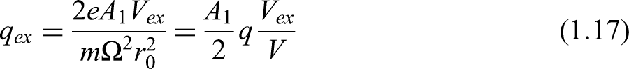
The excitation parameter $q_{ex}$ is proportional to dipolar voltage amplitude $V_x$ (from zero to peak) and equals to

$$q_{ex}={\displaystyle \frac{2e{A}_1{V}_{ex}}{m{\mathrm{\Omega }}^2{r}_0^2}={\displaystyle \frac{A_1}{2}q{\displaystyle \frac{V_{ex}}{V}}}}$$

(1.17)

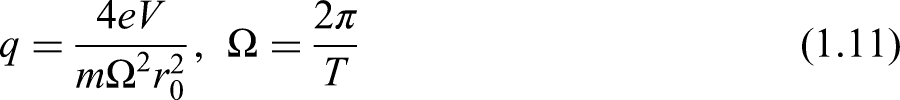
where $A_1\cong 0.8$ is amplitude of the dipolar harmonic, generated by the round rod set in wide region $r/r_0$ $=1.11-1.15$ , r is the rod radius. Knowing the value $q_{ejec}$ , which determines the mass range, we find the value $\beta$ according to the dependence $\beta (q)$ (Figure 10). The parameter $\beta$ determines the resonance frequency $\omega =\beta \mathrm{\Omega }/2$ , where the frequency $\mathrm{\Omega }$ is defined by expression (1.11).

Figure 10.

Dependences of the stability parameter $\beta$ on the parameter q for different wave form shapes: $\tau =0$ (rectangular), $\pi /32$ , $\pi /8$ and $\pi /4$ (triangular).

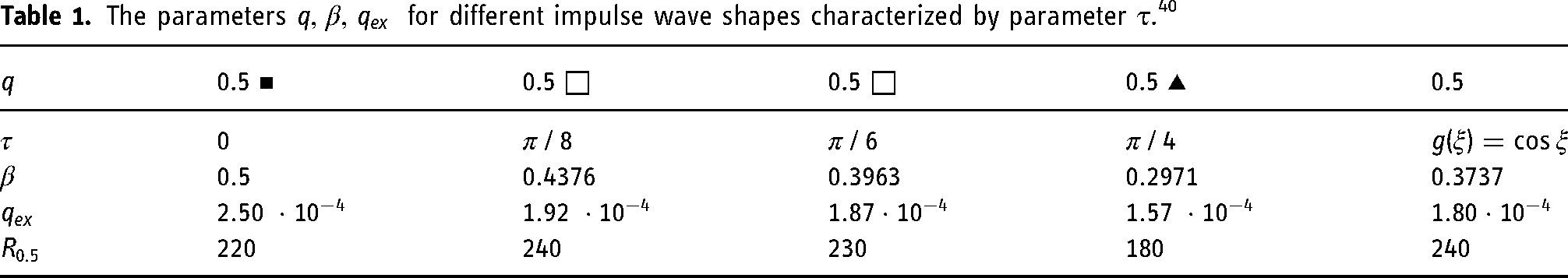
Here we discuss the calculated excitation contours for the conditions, which are presented in Table 1. These data may be useful for the creation the drive RF voltage and the dipolar voltage power supplies and for fundamental search of the process of the resonance ion injection. The trajectory method was used for an ion ensemble with a random distribution of initial positions and velocities with standard deviation ${\sigma }_x=0.01r_0$ and initial velocities with standard deviation ${\sigma }_v=6.3\cdot {10}^{-3}{r}_0\mathrm{\Omega }$ to calculate excitation contours.

Table 1.

The parameters $q,\beta ,q_{ex}$ for different impulse wave shapes characterized by parameter $\tau$ . ⁴⁰

$q$	0.5 ▪	0.5 □	0.5 □	0.5 ▴	0.5
$\tau$	$0$	$\pi /8$	$\pi /6$	$\pi /4$	$g(\xi )=\cos \xi$
$\beta$	$0.5$	$0.4376$	$0.3963$	$0.2971$	$0.3737$
$q_{ex}$	$2.50\cdot {10}^{-4}$	$1.92\cdot {10}^{-4}$	$1.87\cdot {10}^{-4}$	$1.57\cdot {10}^{-4}$	$1.80\cdot {10}^{-4}$
$R_{0.5}$	$220$	$240$	$230$	$180$	$240$

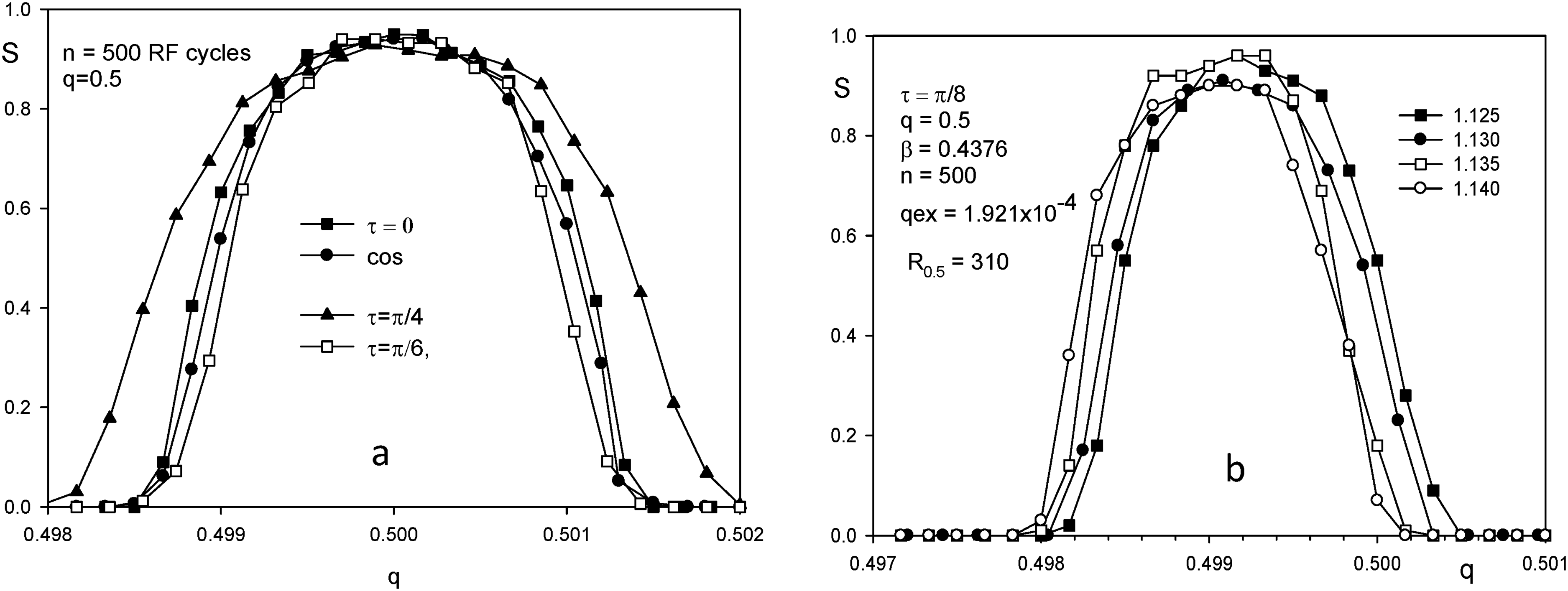
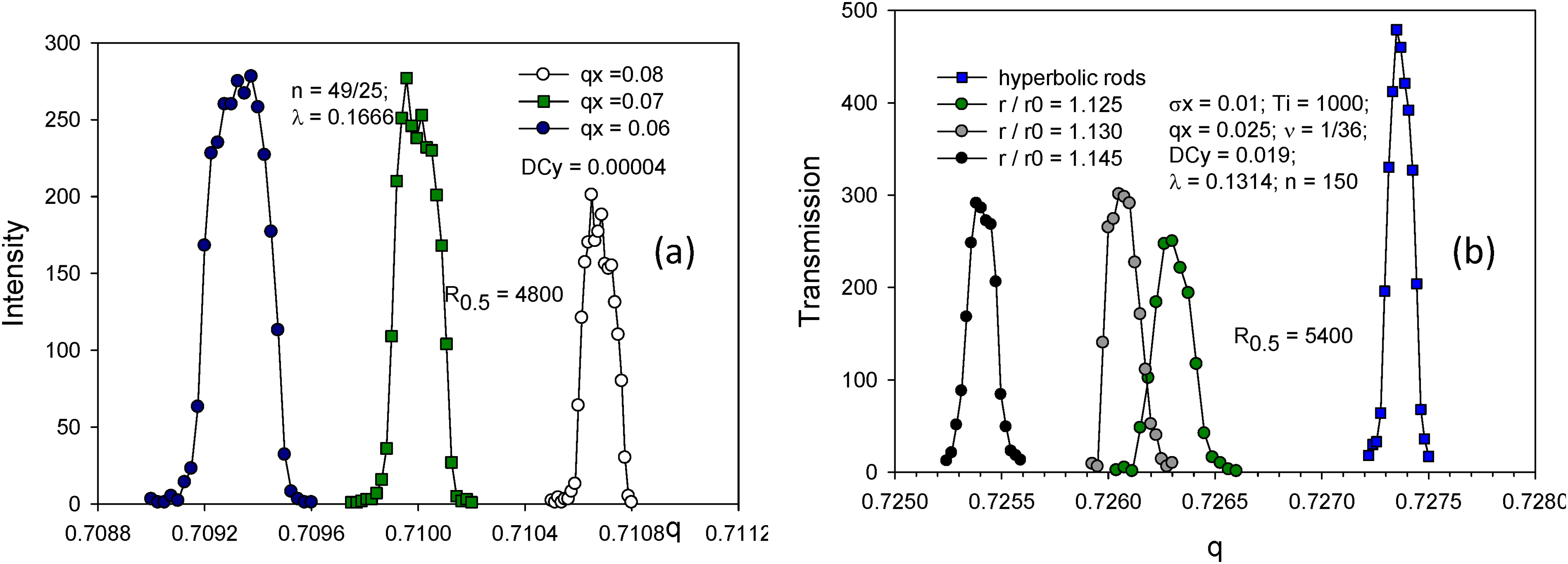
Figure 11 shows contours for two cases: (a) a perfect quadrupole field and (b) rod sets with design parameters $\frac{r}{r_0}=1.125,1.130,1.135$ and $1.140$ . Comparison of the contours for different impulse shapes rectangle wave ( $\beta =0.5$ ), sinusoidal wave ( $\beta =0.3737$ ), trapezoidal wave ( $\beta =0.3963$ ), and triangle wave ( $\beta =0.2971$ ) shows that the triangle wave contour has the lowest resolution. The mass selectivity for the other pulse waves is approximately the same (Figure 11(a)). Excitation time $n=500$ consequents to scan speed $2000$ Th/s for working frequency $1$ MHz. The required amplitudes $q_{ex}$ and the resolution $R_{0.5}$ determined for $50\text{\%}$ peak height are shown on the Table 1. In case of round rods (Figure 11(b)) for all indicated values of $r/r_0$ the resolution is approximately the same, $R_{0.5}\cong 310$ . Use of round rods gives approximately $310/20=1.5$ times gain in resolution compared to hyperbolic electrodes (Figure 11(a)).

Figure 11.

(a) The excitation contours at shown wave shapes at working point $q=0.5$ and excitation time $n=500$ RF cycles, $A_2=1$ . (b) The excitation contours for different rod set ratio $r/r_0$  = 1.125, 1.130, 1.135 and 1.140 for given condition $\tau =\pi /8$ , $q=0.5,\beta =0.4376$ . ⁴⁰

The theoretical resolution $R_{0.5}$ depends on dispersion of q, derivative $d\beta /dq$ , and $\beta$ and is proportional to an excitation time n according to equation (4):

$$R_{0.5}=C{\displaystyle \frac{d\beta }{dq}qn=-Cn{\displaystyle \frac{\cos Q\sinh Q-\sin Q\cosh Q}{\sqrt{8}\sqrt{1-\mathrm{co}{\mathrm{s}}^{2}Q\cos {\mathrm{h}}^{2}Q}}\sqrt{q}}}$$

(1.18)

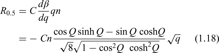
where the constant C is an adjustment parameter depending on the peak level. The dependencies $B(q)q$ (the constant $C=1.0$ for case when peak level is about 96–98%) and $R_{0.5}/n$ which are determined from numerical experiment (simulation) are presented on Figure 12. One can see a good agreement between formula (1.18) and the result of the simulation of the excitation contours with rectangular wave impulse.

Figure 12.

(a) The solid line is theoretical curve $qd\beta /dq$ (equation 1.18) and circle points are results from numerical simulation of the excitation contours. (b) A comparison between theoretical (line) mass resolution and experimental resolution (filled circles) at different values of q for Sin wave. ⁴⁰

At the same time, there is a discrepancy between the theory and experiment at higher ejection q values, which is illustrated in Figure 12(b). In the experiment, the scanning speed was $V_S=2000$ Th/s for all resonance frequencies. The ion excitation time $n=f/V_S=7.68\times 105/2.0\times 103=384$ RF cycles. Such a difference can be explained by the fact that the trapping efficiency decreases with higher values of $q$ ^16,17,19 because the QMF acceptance will decrease with q up to $q=0.908$ .

LIT with round rods

Here we describe the results of a study of the rod's radius optimum ratio r to field radius $r_0$ for excitation and ejection of ions. The design of the linear quadrupole with circular rods is defined by the parameter $\eta =r/r_0$ . The electric field generated by the parallel electrodes allows an analytical description by the complex potential $\phi (z)=A_2{z}^2+A_6{z}^6+A_{10}{z}^{10}+A_{14}{z}^{14}\dots$ . The amplitudes of $A_k$ for a number of values of $\eta$ are given in. ⁴² To calculate the excitation contour, the trajectory method based on the numerical solution of the equations of motion of ions (1.3) and (1.4) is used.

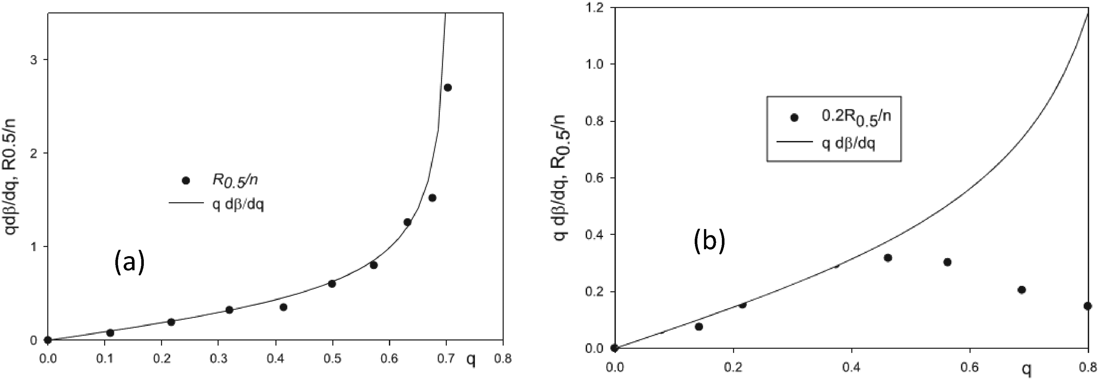
The transmission contours, as the parameter $\eta$ increases (marked with $\eta$ values), are shifted along the q -axis toward lower values (Figure 13(a)). The excitation contours at the resonant frequency $\nu =1-\beta /2$ of the second harmonic are shown in Figure 13(b). The mass peak resolution as $\eta =r/r_0$ changes is presented in more detail in Figure 14 for two values of frequencies $\nu =\beta /2$ and $\nu =1-\beta /2$ .

Figure 13.

Peak shapes for round rod sets with different ratios $r/r_0$ . Dipolar excitation: $q=0.85$ , $n=1000$ rf cycles. Initial conditions: ${\sigma }_x=0.01r_0$ , $T=1000$ K, $500$ trajectories/point. The peak labeled “ q ” corresponds to a pure quadrupole field. (a) $\nu =\beta /2$ and (b) $\nu =1-\beta /2$ . ⁴¹

Figure 14.

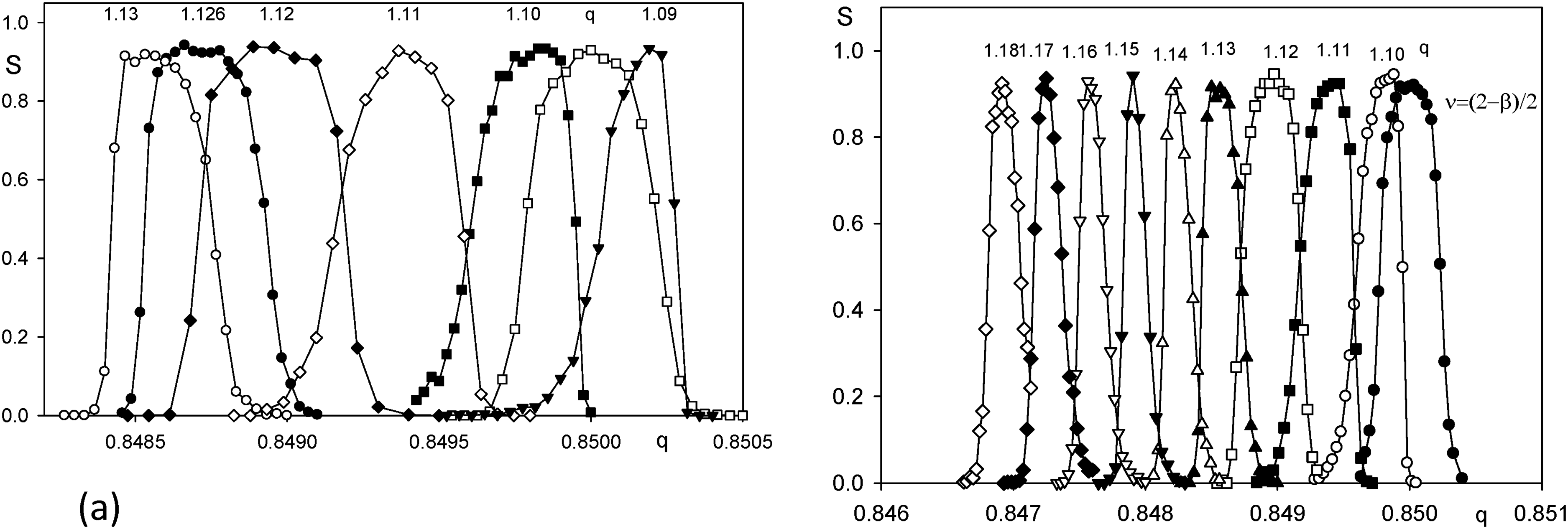
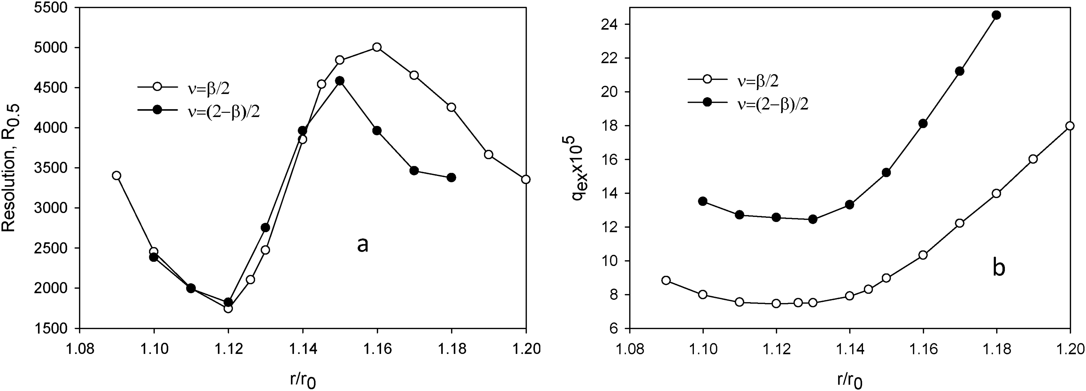
(a) Dependences of the mass resolution $R_{0.5}$ and (b) the required amplitude $q_{ex}$ versus $r/r_0$ for two resonance frequencies $\nu =\beta /2$ and $\nu =1-\beta /2$ . The excitation time is $n=1000$ RF cycles, $q_{ex}=0.85$ . ⁴²

From Figure 14(a) follows that mass resolution reaches its maximum at $\eta =1.16$ . For the mass filter the optimal values of $r/r_0$ are $1.10-1.13$ . ⁴⁴ With excitation for ejection, it can be seen that the ratio $\frac{r}{r_0}=1.1451$ gives higher resolution than the ratio $\eta =1.126$ . Thus, the optimum ratio for ion ejection with DE differs from the optimum ratio for a mass filter. The round rod set with $r/r_0=1.16$ gives an increase in resolution over a pure quadrupole field of $5250/1940=2.7$ times.

Increasing the radius r of the electrodes leads to an increase in the required amplitude $q_x$ of the dipole potential, since the amplitude $A_2$ of the spatial harmonic also increases. Further, since the amplitude of the time harmonic with frequency $\nu =\beta /2$ is greater than for the harmonic with frequency $\nu =1-\beta /2$ (Figure 14(b)), the required value of $q_x$ is also greater. The minimum resolving power for the two frequencies is reached at $\eta =1.120$ , which is caused by a complex change in the spectral composition of ion oscillations.

LIT with quadrupole excitation

Linear ion trap excitation contour with round rods have been studied by numerical methods, in particular, the contour dependence on the geometrical parameter $\eta =r/r_0$ . ⁴³ The ion motion equations for quadrupole excitation by auxiliary AC potential in the field created by circular electrodes have the form

$${\displaystyle \frac{d^{2}x}{d{\xi }^2}=-[q\cos (2(\xi -{\xi }_0))+q_{ex}\cos [2\nu (\xi -{\xi }_0)+2\alpha ]]{\displaystyle \frac{\mathrm{\partial }}{\mathrm{\partial }x}Re[\phi (z)]}}$$

(1.19)

$${\displaystyle \frac{d^{2}y}{d{\xi }^2}=-[q\cos (2(\xi -{\xi }_0))+q_{ex}\cos [2\nu (\xi -{\xi }_0)+2\alpha ]]{\displaystyle \frac{\mathrm{\partial }}{\mathrm{\partial }y}Re[\phi (z)]}}$$

(1.20)

Here the dimensionless variables $q,\xi$ are the same as in equations (1.5), $q_{ex}$ is the dimensionless amplitude of the auxiliary quadrupole AC potential, and $\nu =\omega /\mathrm{\Omega }$ is the dimensionless frequency. Three methods of quadrupole excitation are considered. This excitation can be achieved by auxiliary AC quadrupole potential, amplitude, and frequency modulation of the RF drive voltage.

For comparison, the mass peaks for quadrupole amplitude excitation (AM) and DE are shown in Figure 15. The ejection parameter $q_{ejec}=0.862883$ , resonance frequency $\nu =\omega /\mathrm{\Omega }=\beta =4/5$ , excitation time $n=500$ . The comparison shows that DE is more effective $(R_{0.5}=960)$ than quadrupole excitation $(R_{0.5}=450)$ . Perhaps this difference is due to the fact that with quadrupole excitation the forcing resonance force is proportional to the ion displacement ( $F_{ex}\sim x$ ), while with DE, the forcing force is independent of the ion position. The LIT with round rods shows an even greater gain in resolving power, up to twofold ( $R_{0.5}=1900$ ).

Figure 15.

Excitation contours for two methods of resonance effect on ions: quadrupole with amplitude modulation (AM) and dipole excitation (DE) and for a trap with hyperbolic and cylindrical electrode: ● AM ( $R_{0.5}=450)$ ; ○ DE, ( $R_{0.5}=960$ ); □ $\mathrm{DE},\eta =1.15(R_{0.5}=1900);$ AM, $r/r_0=1.15$ ( $R_{0.5}=960$ ). ⁴³

Figure 16 illustrates the effect of the octupole component $A_4$ on the mass selectivity of LIT with a quadrupole additive potential. Increasing $A_4$ gives a shift of the mass peak along the q -axis. The resolution reaches a maximum of $R_{0.5}=1190$ at amplitude $A_4=0.05$ of the spatial field harmonic. An addition of a small octupole component with $A_4=0.005-0.01$ allows to increase the resolution power $R_{0.5}$ approximately twofold compared with ideal quadrupole field.

Figure 16.

Effect of the amplitude $A_4$ of the octupole field component on the shape of the mass peak $S(q)$ . ○ $A_4=0$ (pure field), $R_{0.5}=420$ ; ● $A_4=0.0025,R_{0.5}=270;◻-A_4=0.004,R_{0.5}=800;$ ▪ $A_4=0.005,R_{0.5}=1190;$ ● (a) $A_4=0.01$ , $R_{0.5}=1160$ . $\nu =\beta =4/5$ , n = 500. ⁴³

Quadrupole excitation can be applied with amplitude or frequency modulation of the main RF voltage, or with an auxiliary excitation AC potential. A continuous separation mode based on the above quadrupole excitation methods was considered in reference. ⁴⁵ For this mode of operation, the excitation time is the flight time of ions through the filter and this must be sufficient to resolve ions with the desired resolution. The quadrupolar resonance excitation takes place on the frequencies $\nu =1/5,2/5$ and $3/5$ .

Excitation by an auxiliary quadrupole signal of frequency $\nu$ does not influence the form and position of a mass peak (Figure 17 (a)) in contrast to the dipole effect. Frequency excitation (Figure 17(b)) creates symmetrical contours; their positions are determined by frequency $\nu =1/5$ and $\nu =2/5,3/5$ . Here $m_a$ and $m_f$ are indexes of amplitude and frequency modulation (see equations 3.14, 3.17). The same pattern is observed for the amplitude modulation, which is shown in Figure 17(c). The resolutions $R_{0.5}$ for each excitation method are approximately the same for this excitation time. The difference between using auxiliary excitation and the modulation methods may be related to the different excitation frequency spectra: with an auxiliary signal, the RF voltage contains two harmonics; with amplitude modulation, three harmonics; and with frequency modulation, more than three harmonics.

Figure 17.

Excitation contours with excitation frequencies $\nu =1/5,2/5$ and $3/5$ . Ejection parameter $q_{ejec}=0.73243(\beta =4/5)$ . (a) Auxiliary excitation, (b) frequency modulation and (c) amplitude modulation. Excitation time $n=1000$ cycles. ⁴⁵

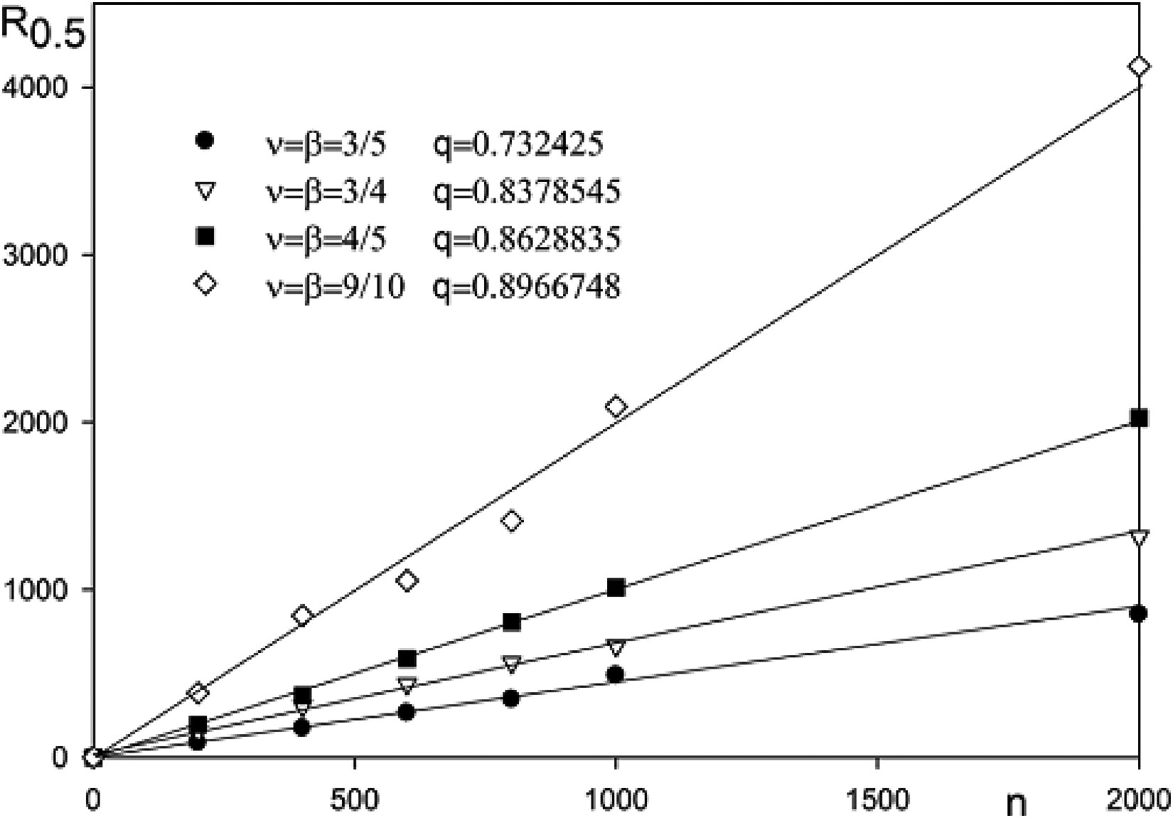
Figure 18 illustrates linear dependence of the mass resolution R, defined at half-peak height, on the excitation time n. As the ejection parameter q increases, the mass selectivity of resonant excitation increases. The dependence $R_{0.5}(n)$ has the same character for all excitation methods.

Figure 18.

Amplitude modulation. ²⁹ Resolution $R_{0.5}$ vs. excitation time n for different ejection values q and different resonant excitation frequencies $\nu$ . ⁴⁵

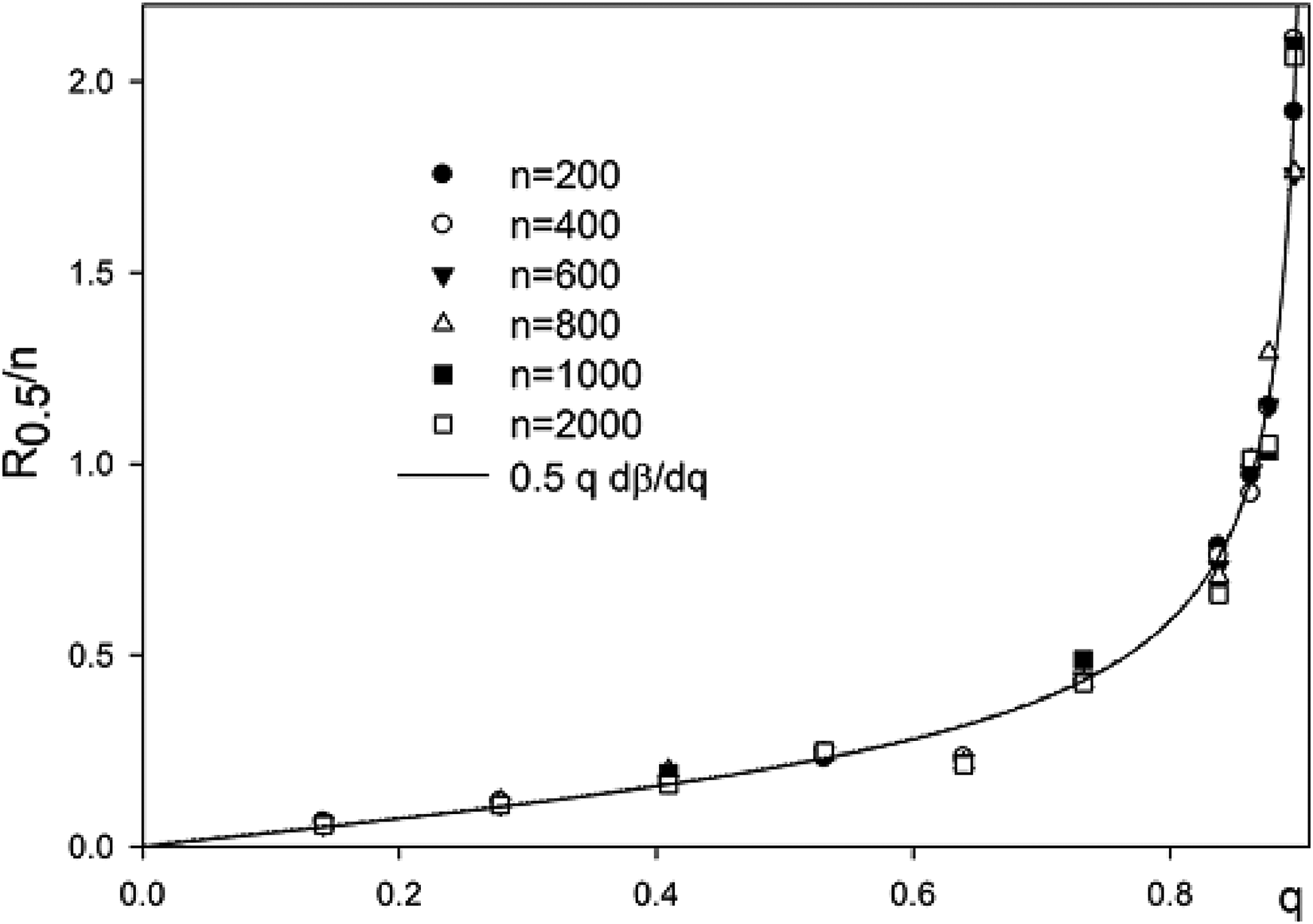
The calculation of the excitation contours allows us to find the dependence of the ratio of $R_{0.5}$ to the excitation time n, $R_{0.5}/n$ on the parameter q at the excitation frequency $\nu =\beta$ . Figure 19 shows the dependences of the ratio $R_{0.5}/n$ on the operating parameter q for excitation time n. For quadrupole excitation at given values of q and $\beta$ excitation frequencies are $\nu =1/P,2/P,$ …, $L/P$ , $L/P<1$ , L and P are integers. Therefore, several points on the curve $R_{0.5}/n(q)$ are indicated for some values of q. With DE, the resolution in a simple approximation is given by formula (1.4). For comparison, the theoretical dependence $0.5q(d\beta /dq)$ is also shown in Figure 19. One can see an excellent agreement between theory and simulation results for quadrupole and DE (Figure 12(a), Figure 19). In practice, at larger values of the ejection parameter q, the resolution decreases (Figure 12(b)). The reason for this discrepancy is due to the fact that at the boundary values of q, when the derivative $d\beta /dq$ gets larger, the acceptance of the RF quadrupole decreases. The simulation assumes that all ions should be concentrated on the quadrupole axis with ${\sigma }_x=0.01r_0$ , which is achieved by precooling in a buffer gas. At high axial ion concentration, the resolution drops due to the manifestation of a spatial charge. The large size of the ion cloud results in a noise pedestal of the mass peak. At a given scanning speed, the resolution is directly proportional to the RF field frequency. Therefore, when working at boundary values of q, it is necessary to use higher frequencies, which leads to a reduction in the range of analyzed ion masses.

Figure 19.

Comparison of the theoretical curve $0.5qd\beta /dq$ and the numerical simulation curve $R_{0.5}/n$ vs. the excitation parameter q. Excitation frequency $\nu =\beta$ . ⁴⁵

Operation in the second stability region

In principle, it is possible to realize mass-selective excitation of ion oscillations at any point $(a,q)$ of the second stability region (Figure 20). In the presence of the quadrupole DC potential, the working points lie on the scanning line $=2\lambda q$ inside the stability region. The LIT operates usually RF only mode when $a=0$ and the working points are located along the q -axis. This is a major advantage of the LIT mode of operation compared to the quadrupole mass filter.

Figure 20.

The second stability region on $a,q$ plane. The dashed lines are iso- $\beta$ lines. The working points are shown: $a=0,q=7.752(\beta ={\beta }_x={\beta }_y=1.2);a=0,q=7.547(\beta ={\beta }_x={\beta }_y=1.5);a=0,q=7.5735(\beta ={\beta }_x={\beta }_y=1.8);a=0.011,q=0.7547,({\beta }_x=1.6,{\beta }_y=1.3575)$ . Strait line $a=2\cdot 7.324{10}^{-4}q$ is the scan line. ⁴⁶

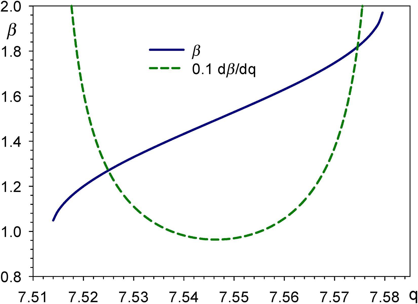
The resolution of DE is controlled by the function ${\beta }^{\mathrm{\prime }}(q)$ , which is important for the mass selectivity of DE. Figure 21 shows the dependence of $\beta (q)$ and its derivative ${\beta }^{\mathrm{\prime }}(q)$ . As q approaches the boundaries of the second stability region, ${\beta }^{\mathrm{\prime }}(q)$ increases sharply, but the linear trap acceptance decreases to zero.

Figure 21.

Function $\beta (q)$ and its derivative ${\beta }^{\mathrm{\prime }}(q)$ in the second stability region. ⁴⁶

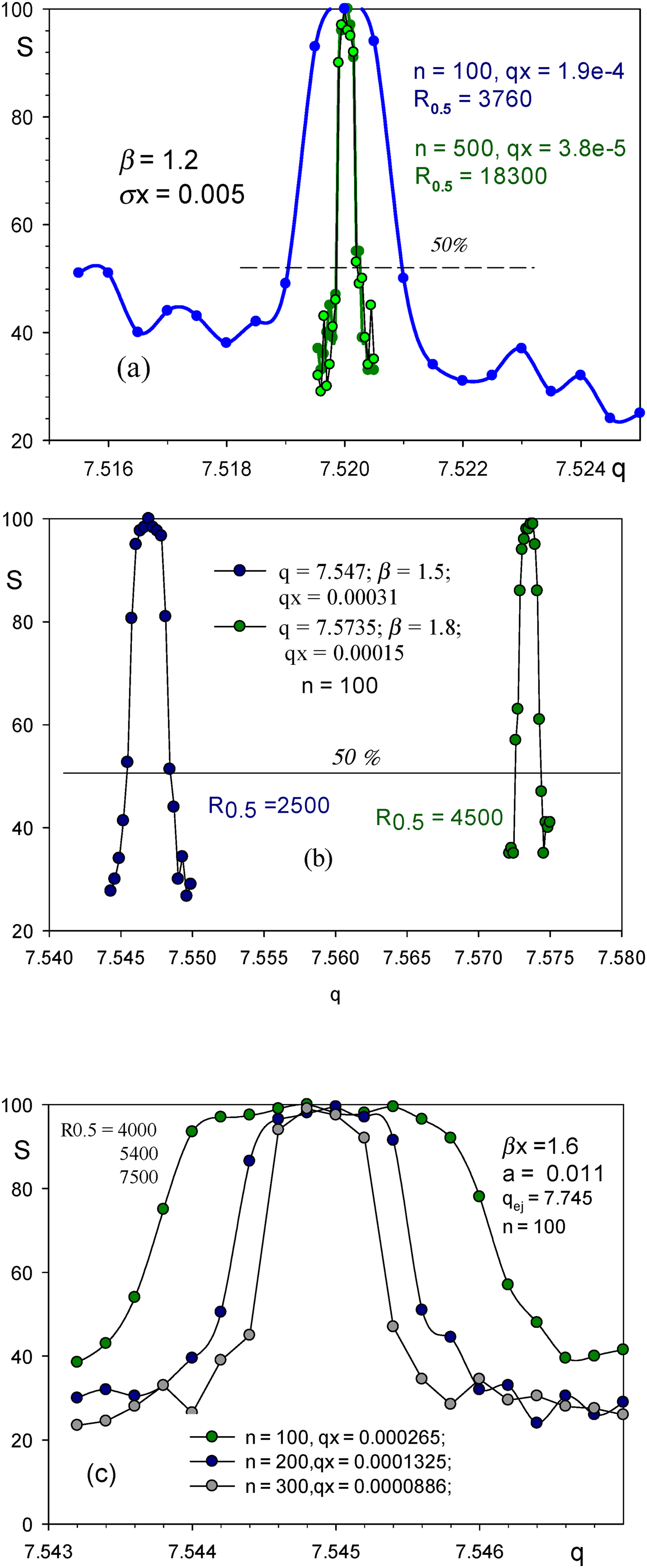
Figure 22 shows the excitation contours at the operating points marked in Figure 20. For each contour, the values of excitation time n, excitation amplitude $q_x$ , and resolution $R_{0.5}$ are given. Let us compare the resolution for contours (a) $R_{0.5}=3760$ , (b) $R_{0.5}=2500$ , and (c) $R_{0.5}=4000$ for $n=100$ . The resolution increases then the operating point q approaches the boundaries of the second stability region, as the derivative $d\beta /dx$ (Figure 21) and the resolution $R\sim q\frac{d\beta }{dx}n$ increase also. Near the left boundary, the contour has an asymmetric pedestal (Figure 22(a)).

Figure 22.

Excitation contours at operating points (a) $q=7.52$ ( ${\beta }_x=1.2);(b)q=7.5735$ ( ${\beta }_x=1.8);$ (c) $q=7.545,a=0.011$ ( ${\beta }_x=1.6$ ). ${\sigma }_x=0.005$ . ⁴⁶

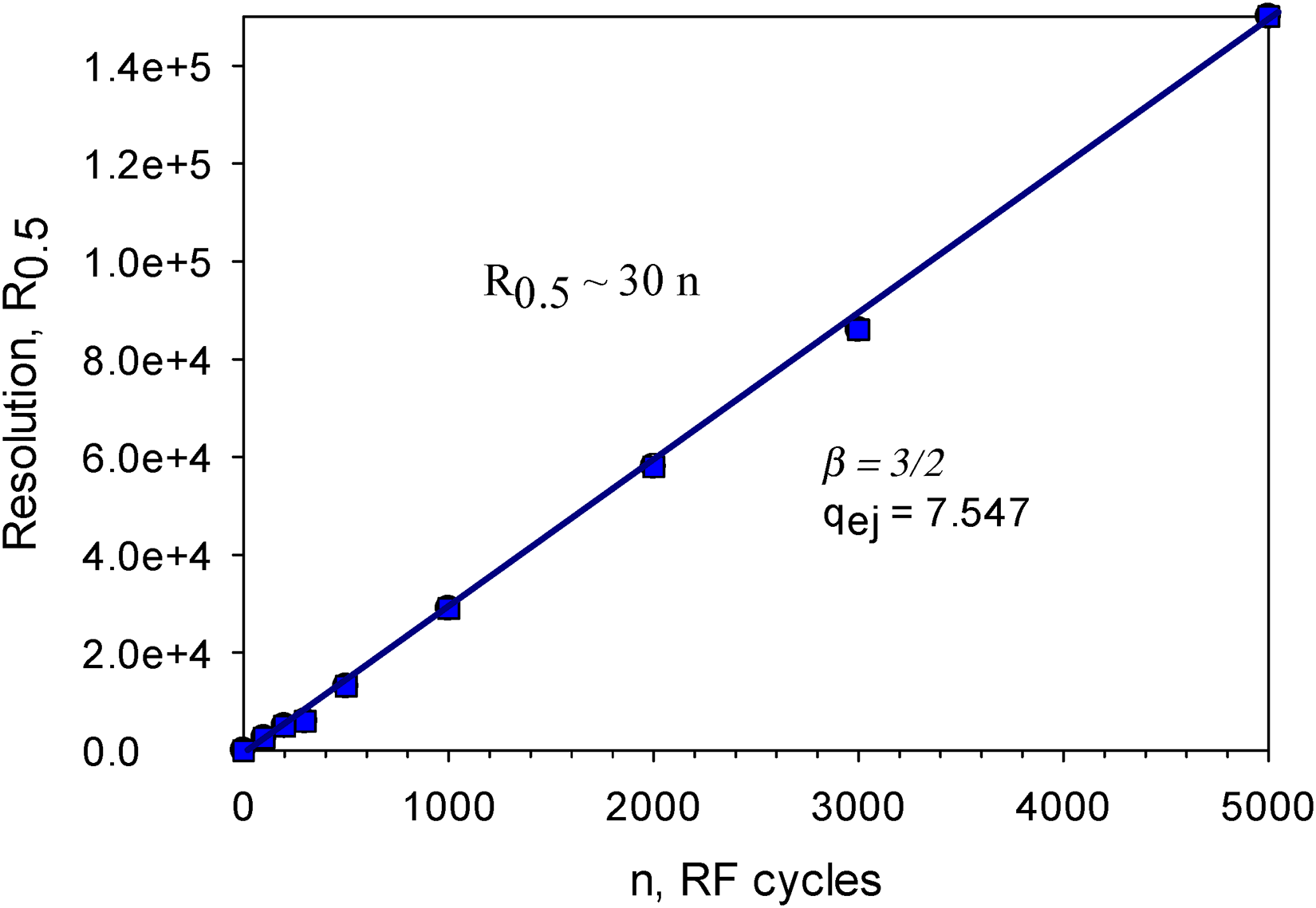
The linear dependence of the resolution masses $R_{0.5}$ on the excitation time n is shown in Figure 23 at the operating point $q=7.547$ , in which the derivative is equal to $d\beta /dx=0.965$ . For the constant C, the resolution is $R_{0.5}=0.965Cqn=7.28Cn$ . From the graph of Figure 23, we find the straight line equation $R_{0.5}\cong 30n$ and $C=4.1$ . For the first stability region $q_{ejec}=0.85$ and the resolution $R_{0.5}\cong 1.63n$ . ³³ The resolution for the second stability region is 30/1.63 $\cong$ 18 times higher compared with the first stability region.

Figure 23.

Linear dependence of the resolution $R_{0.5}$ on the excitation time n for $=3/2,$ $q_{ej}=7.5469$ . ${\sigma }_x=0.005r_0$ . ⁴⁶

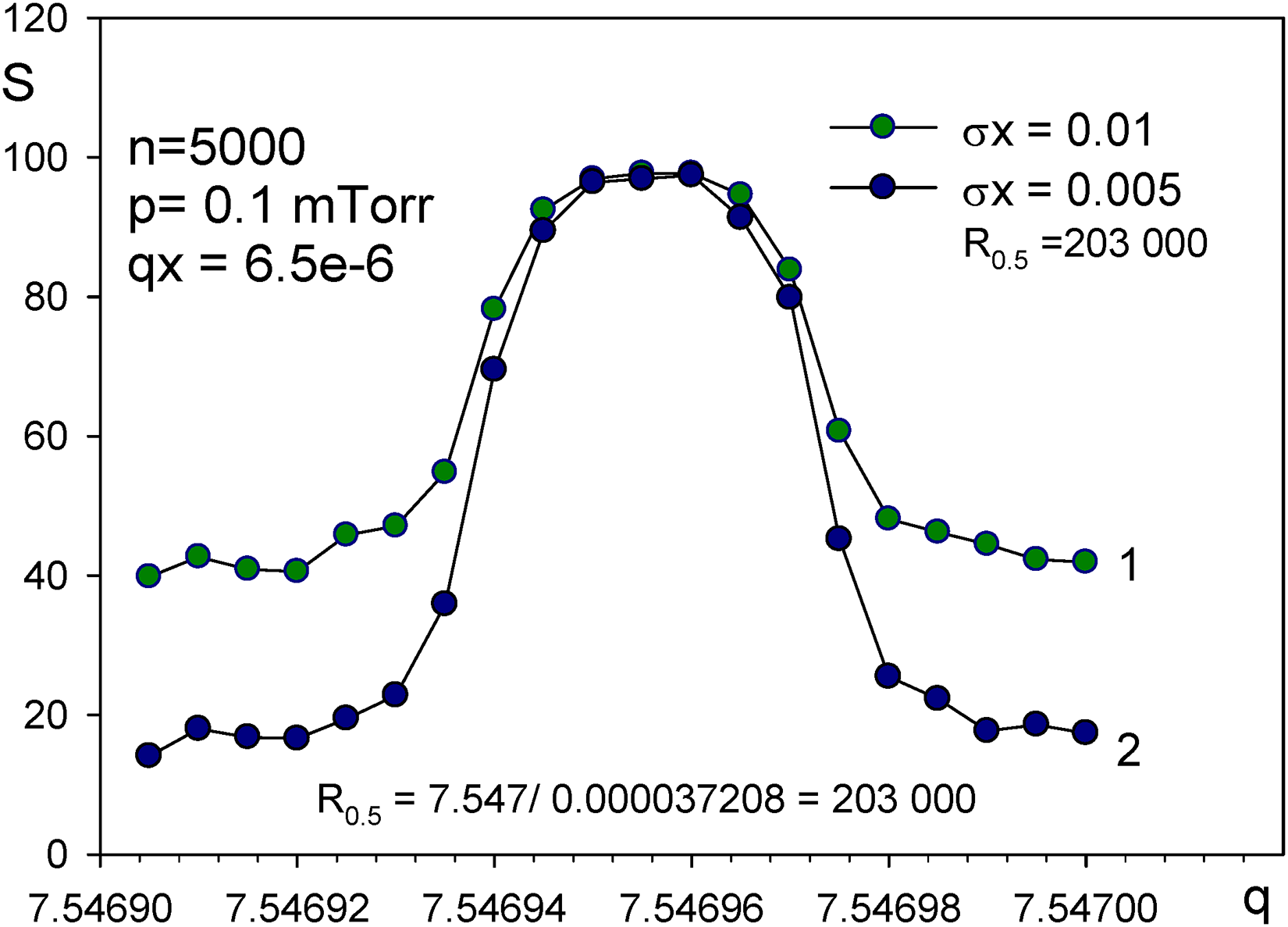
An excitation contour with high resolution $R_{0.5}\cong 200,000$ and 100% ( $S\cong 100$ ) excitation efficiency is illustrated in Figure 24 (curve 2). The presence of a small buffer gas pressure $p=0.1$ mTorr results in a 25% increase in resolution compared to the case with no gas damping. The noise pedestal also decreases with increasing pressure. Increasing the near-axis ion concentration ${\sigma }_x=0.005$ decreases the noise pedestal and increases the resolving power in the presence of pressure. In the simulation, the quadrupole field was assumed to be ideal, and the spatial ion charge was not taken into account.

Figure 24.

Excitation contour for slow scan speed 100 Th/s ( $n=5000$ ) and small damping gas pressure $p=0.1\mathrm{mTorr}$ . Dipole amplitude $q_x=6.05{10}^{-6};$ $(1){\sigma }_x=0.01;(2){\sigma }_x=0.005$ . ⁴⁶

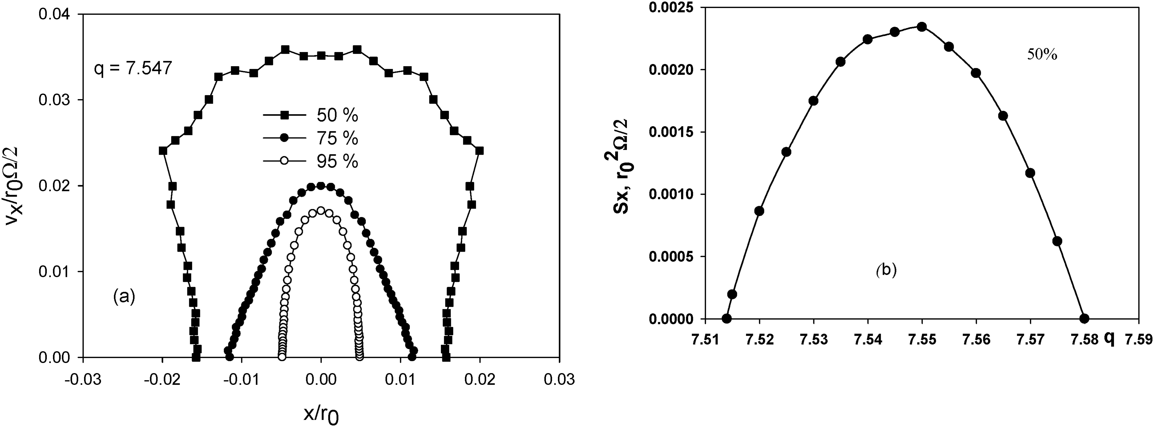
The filling of the trap with ions and the formation of the ion cloud near the quadrupole axis is controlled by the quadrupole acceptance. The LIT acceptance is represented at the operating point $q=7.547$ by contours defined by 50, 75, and 95% transmission levels (Figure 25(a)). When simulated, the radial distribution of ions before emission is described by the standard deviation ${\sigma }_x=0.01r_0$ and ${\sigma }_x=0.005r_0$ (Figure 24). At ${\sigma }_x=0.01r_0$ , the excitation contour has a 40% noise pedestal. Such value of ${\sigma }_x$ corresponds to 75% transmission level. The value ${\sigma }_x=0.005r_0$ gives a noise pedestal of 20% and corresponds to 95% capture level.

Figure 25.

(a) Acceptance of the LIT at the operating point $q=7.547$ , characterized by transmission contours determined from 50%, 75%, and 95% transmittance levels. (b) LIT acceptance (50% contour area) as a function of the excitation parameter $q$ .

As the ejection point q approaches the boundaries of the second stability region, the derivative $d\beta /dq$ increases (Figure 21) and so does the resolving power. However, this increase in resolution is limited by the LIT acceptance, when the phase area $S_x$ decreases quadratically as q approaches the boundary values $q=7.514$ and $q=7.58$ . This dependence of $S_x(q)$ is shown in Figure 25(b). Note that $S_x(q)=S_y(q)$ at $a=0$ . Phase volume (area) of acceptance is proportional to $\pi r_0^{2}F$ , where $r_0$ is the field radius and F is the cyclic frequency of RF oscillator. Therefore, it is more effective to use LIT with a larger electrode radius.

Dual-frequency resonant excitation

D. Snyder and R.G. Cooks proposed a new method for eliminating the influence of the ion spatial charge on the quality of the LIT mass spectrum using two-frequency excitation of ion oscillations. ⁴⁷ The presence of a spatial charge leads to a broadening and displacement of the mass peak on the mass number scale. ⁴⁸

Based on the spatial charge model of the ion trap,^48,49 using the trajectory method to modeling an excitation contour, taking into account the influence of the buffer gas pressure, the process of dipole dual-frequency excitation of ion oscillations was studied. ⁵⁰ Numerical simulations have shown that the use of dual-frequency excitation eliminates mass shift on the mass number scale and increases resolution when the frequency difference is small $\mathrm{\Delta }f\ll f_1,f_2$ ( $\mathrm{\Delta }f\approx 2.5kHz$ ) and the phase difference of two harmonic signals is $0-\pi /3$ at a linear charge density of 50 000/ $r_0$ .

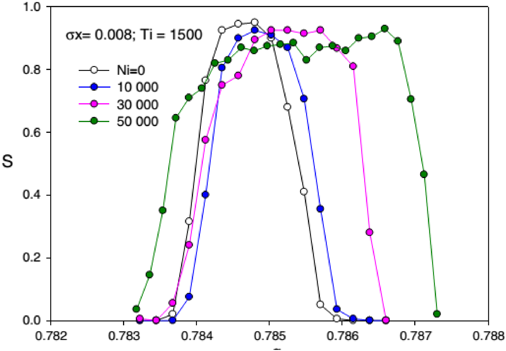
Figure 26 illustrates the effect of the spatial charge, characterized by the linear charge density $N_i$ , on the shape of the mass peak of the linear trap. Increasing the density to $N_i=10,000$ shifts the contour slightly along the q -axis without changing its shape. At a spatial charge density of $N_i=30,000,$ the contour is broadened and shifted. Strong broadening and displacement of the contour's center of “mass” is observed already for $N_i=50000$ .

Figure 26.

Excitation contours at the same frequency and specified values of linear density $N_i$ is number of ions/ $r_0$ ; ${\sigma }_x=0.008$ ; $T_i=1500K$ . ⁵⁰

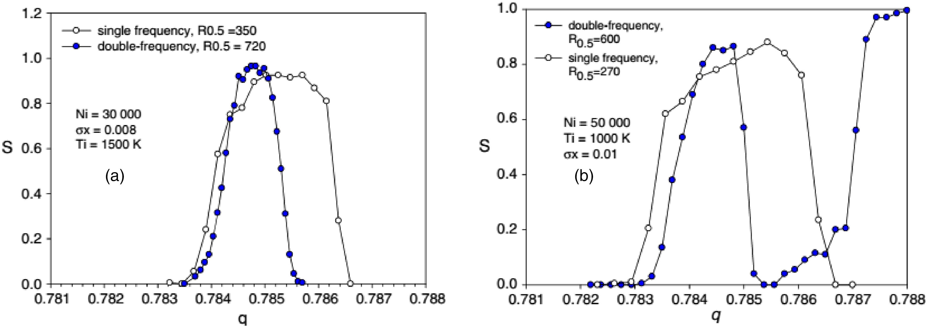
Figure 27 shows the excitation contours for two values of linear charge density: (a) $N_i=30,000$ and (b) $N_i=50,000$ . In Figure 27(a), two peaks for single-frequency and dual-frequency excitation are shown. The influence of the spatial charge is completely eliminated while the resolution is doubled. Figure 27(b) also shows that the contour shape is completely restored and the resolution increases twofold.

Figure 27.

The effect of two-frequency excitation on a trap circuit with a linear charge density (a) $N_i=30,000$ $(\alpha =7\pi /22$ ) and (b) $N_i=50,000$ . Amplitudes of the two dipole signals $q_1$  = 0.00018, $q_2$ = 0.00025, frequency difference $\mathrm{\Delta }f=f\mathrm{\Delta }\beta /2=25$ kHz, $q_{ejec}=0.78427$ ( $\beta =2/3$ ). ⁵⁰

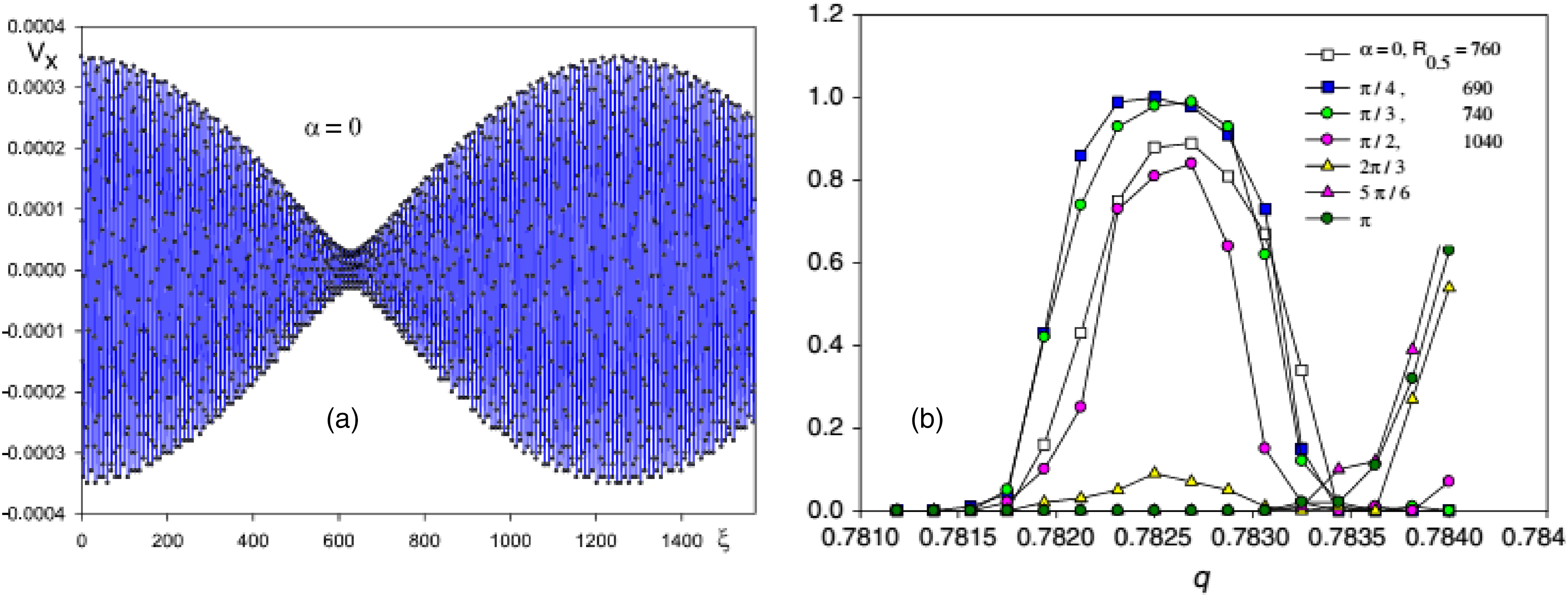
The resulting signal at simultaneous influences on the ensemble of ions represents beats (Figure 28(a)). The form of beats significantly depends on the phase difference of the two sinusoidal signals. The effect of phase differences is taken into account only when modeling and control of the phase difference in the experiment is difficult. As a result, the shape of the contour depends heavily on the phase difference. Good resolution occurs when $\mathrm{\Delta }\beta =0.004$ and the beat packet duration is $n=500$ RF cycles. This corresponds to a scan rate $V_s=1Th\cdot F/n=2000$ Th/sec. Note that the direct and inverse mass-selective sequential excitation can produce different quality mass peaks. Thus, in Figure 28(b) with direct scanning only the left peak will be visible, the second right one is a consequence of the simulation. The second peak disappears because all resonant ions are ejected in the first peak.

Figure 28.

(a) The form of the excitation two-frequency signal at phase difference α=0. (b) Influence of the phase shift $\alpha$ on the excitation contour, $r/r_0=0.140$ . ⁵⁰

The spatial charge effect is reduced by the competition between the two resonant processes with close frequencies due to the phase difference and the synchronization of oscillations in the nonlinear fields of ion oscillations in the low-frequency band of the resonant signal. The use of two resonant forces with two close frequencies results in two processes: excitation of ions of one mass at the first frequency or removal of that mass by resonant excitation at the second, regardless of whether this excitation is sequential or simultaneous.

Quadrupole mass filter with dipole excitation

The first stability region

The possibility of using additional DE for mass analysis of the linear quadrupole is considered in.^51–57 The QMF with DE is described in the patent [(a)]. The idea of the method is to change the stability boundaries of the first region by removing the stable boundary by DE. Dipole resonance excitation of ions creates instability bands that follow along iso-β lines, where β is the characteristic exponent (stability parameter).

The equations of ion motion and the justification of the stability diagram of the quadrupole mass filter (Figure 29) can be found in the book. ³ Here we do not take into account the end fringing fields of the QMF, since they practically do not affect the process of DE.

Figure 29.

Diagram of the first stability region on the plane of parameters a and q. The lines ${\beta }_y=0$ and ${\beta }_x=1$ are the boundaries of the first area. The lines ${\beta }_x=0.5$ and ${\beta }_y=0.5$ are the instability bands corresponding to the excitation frequencies ${\nu }_x={\nu }_y=0.25,$ $a=2\lambda q$ is the scan line, $\lambda =0.166$ . ⁵⁵

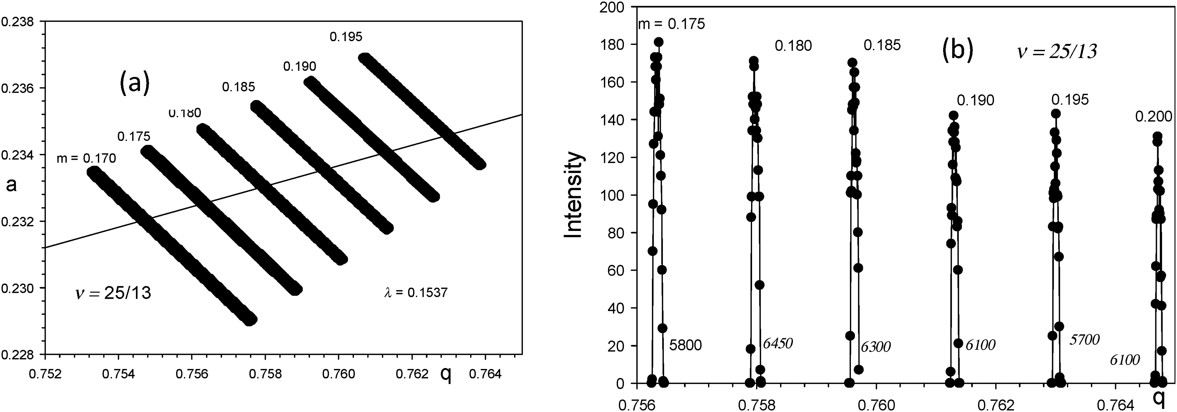
Figure 29 shows the first stability region, bounded by the isolines ${\beta }_y=0$ and ${\beta }_x=1$ . The scan line $a=2\cdot 0.166q$ crosses a small region near the working tip, when ${\beta }_y$ is small and ${\beta }_x$ is close to 1. Resonant frequencies are ${\nu }_x={\nu }_y=0.25$ for $q=0.6407\mathrm{and}a=0$ . Further, at these frequencies, the DE creates instability bands along the isolines ${\beta }_x={\beta }_y=\mathrm{0.5.}$ This means that at any point ( $a,q)$ in the stability region resonance excitation at frequencies ${\nu }_x=1/2{\beta }_x(a,q)$ or ${\nu }_y=1/2{\beta }_y$ $(-a,q)$ can be achieved.

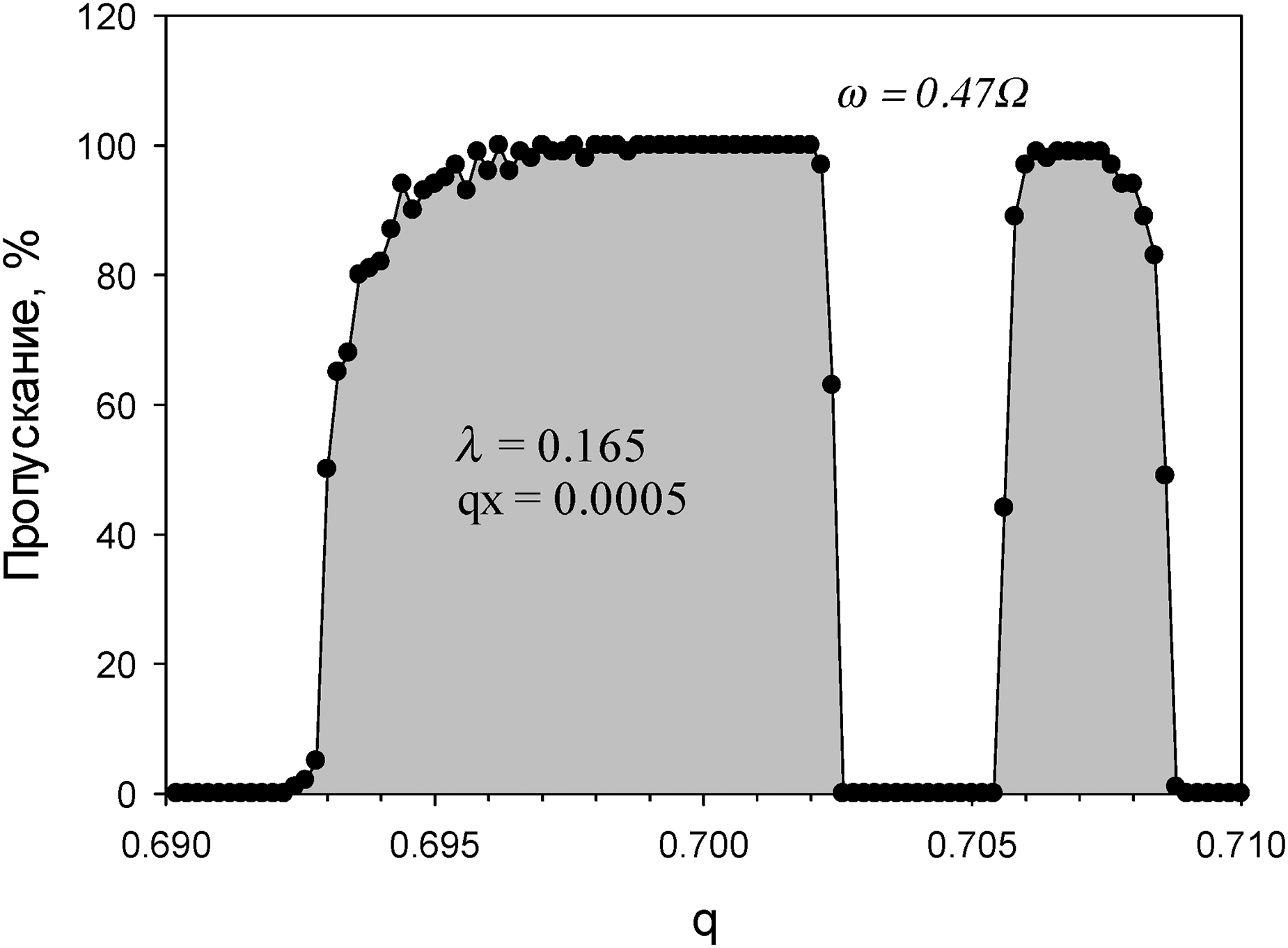
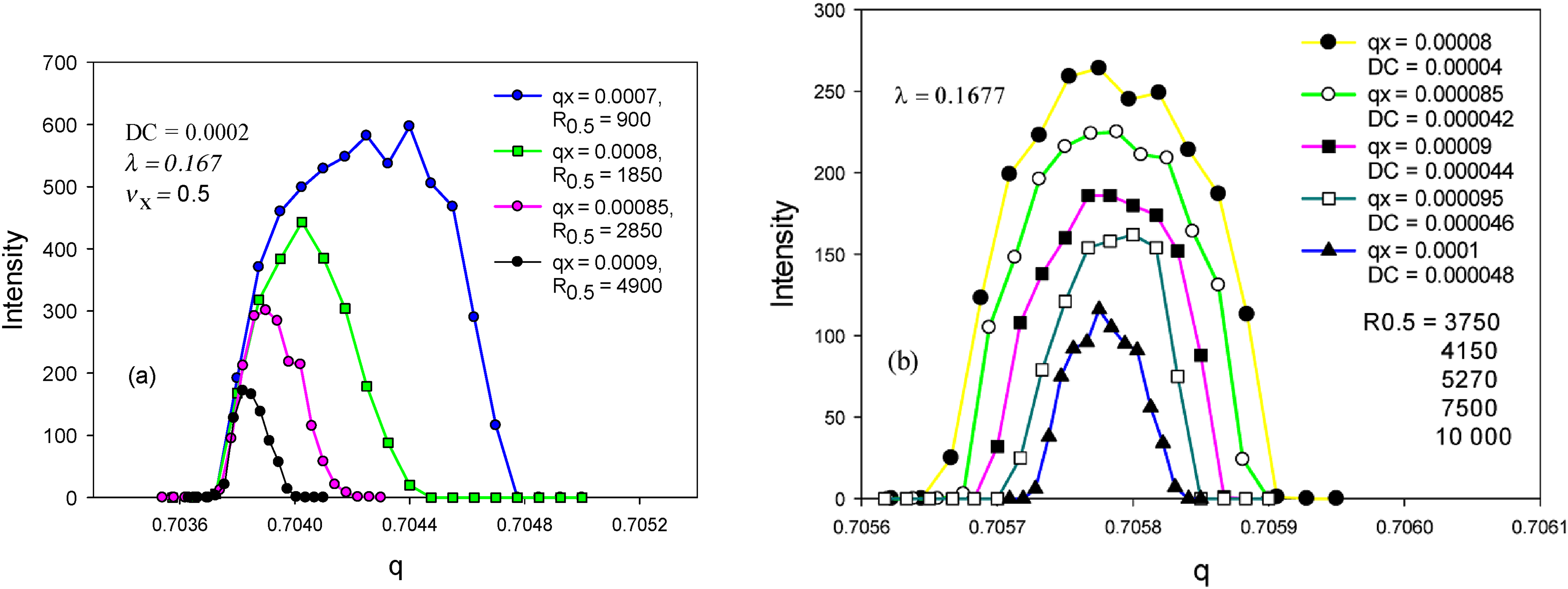
Figure 30 shows the transmission contour (mass peak) with a 100% dip. The dip is due to the instability band ${\beta }_x=0.94$ in the stability diagram (Figure 1), caused by DE with frequency ${\nu }_x=0.47$ . The width of the instability band is $\mathrm{\Delta }q\cong 0.0026$ . The resolution of the original peak is $R=33$ . The left part of the peak can be removed by increasing the amplitude $q_y$ , and we get resolution $R=q/\mathrm{\Delta }q\cong 0.706/0.0035=200$ at 100% transmission. Increasing the amplitude $q_x$ decreases the intensity of the right peak for larger values of the scan parameter $\lambda$ .

Figure 30.

Transmission contour (mass peak) with dipole excitation at frequency ${\nu }_x=0.47$ and amplitude $q_x=0.0005$ . The scan parameter $\lambda =0.165$ . ⁵⁵

Ion oscillation spectrum

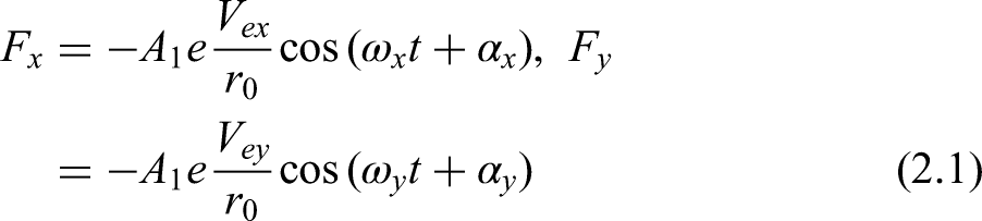
Dipole potentials are applied to the opposite pairs of X and Y electrodes of the mass filter, which play the role of flat capacitors. ⁵¹ As a result, under certain conditions, the ion will be subjected to forces $F_x$ and $F_y$

$$F_x=-A_{1}e{\displaystyle \frac{V_{ex}}{r_0}\cos ({\omega }_{x}t+{\alpha }_x),F_y=-A_{1}e{\displaystyle \frac{V_{ey}}{r_0}\cos ({\omega }_{y}t+{\alpha }_y)}}$$

(2.1)

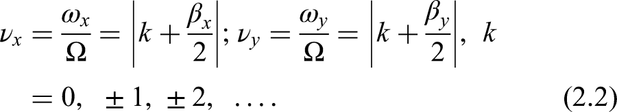
where $A_1=0.798$ is the amplitude of the dipole spatial harmonic, ³² e is the ion charge, $V_x$ and $V_y$ are the amplitudes of the auxiliary voltages, ${\omega }_x$ and ${\omega }_y$ are the resonant frequencies, and ${\alpha }_x$ and ${\alpha }_y$ are the phase shifts between the main QMF supply voltages $\pm (U-Vcos\mathrm{\Omega }t)$ and dipole signals. The minus sign of U corresponds to the Y electrode, and the plus sign to the X electrode for positive ions. The resonant frequencies ${\omega }_x$ and ${\omega }_y$ are chosen on the basis of the spectrum of frequencies ${\nu }_x$ and ${\nu }_y$ for own ion oscillations:

$${\nu }_x={\displaystyle \frac{{\omega }_x}{\mathrm{\Omega }}=\left|k+{\displaystyle \frac{{\beta }_x}{2}}\right|;{\nu }_y={\displaystyle \frac{{\omega }_y}{\mathrm{\Omega }}=\left|k+{\displaystyle \frac{{\beta }_y}{2}}\right|,k=0,\pm 1,\pm 2,\dots .}}$$

(2.2)

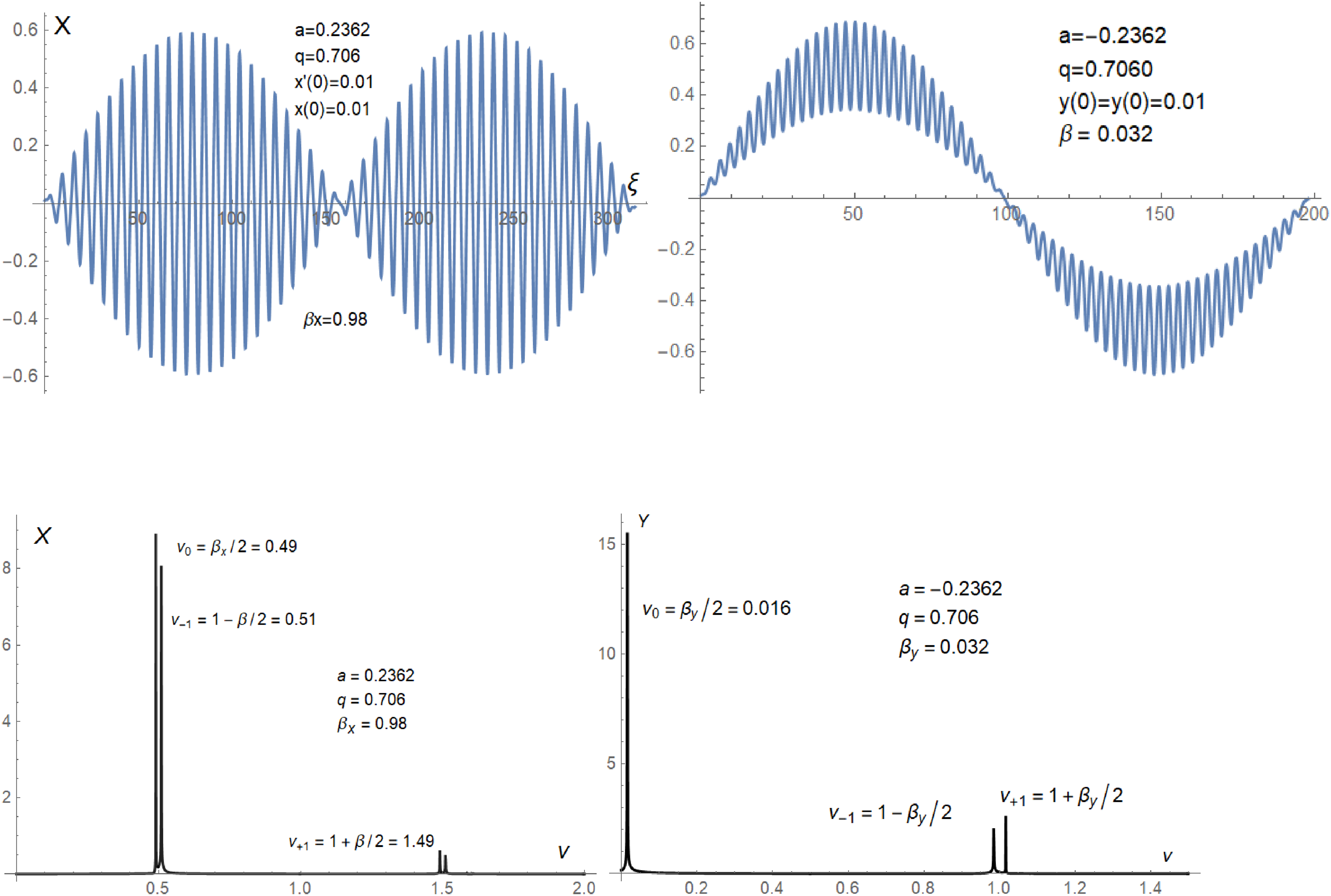
Figure 31 shows the trajectories and spectra of oscillations of ions in perfect quadrupole field at the operating point $a=0.2362,q=0.706$ . The oscillations along the X coordinate have the form of beats at close frequencies ${\nu }_x={\beta }_x/2$ and ${\nu }_x=1-{\beta }_x/2$ with approximately equal amplitudes. Therefore, these frequencies can be used for resonance excitation of ions. The main harmonic of the ion oscillations along the Y coordinate has a low frequency and the largest amplitude. A doublet of harmonics with frequencies ${\nu }_{-1}$ and ${\nu }_{+1}$ , which also form beats, is superimposed on the oscillations of very low frequencies. Resonant excitation requires frequencies $\nu$ whose amplitude is maximal. For this purpose, the spectra are given near the working tip, when ${\beta }_x\le 1$ and ${\beta }_y\ge 0$ . For the working point $a=0.2362,q=0.706$ the values of $\beta$ parameters are ${\beta }_x\cong 0.98$ and ${\beta }_y\cong 0.032$ . For X oscillations ${\nu }_x=0.49,0.51$ and $1.49$ . For Y oscillations ${\nu }_y=0.016,0.984$ and 1.016.

Figure 31.

Ion trajectories and frequency FFT spectrums for X and Y directions at $a=0.2362,q=0.706$ near the stability region tip.

Ion motion equations

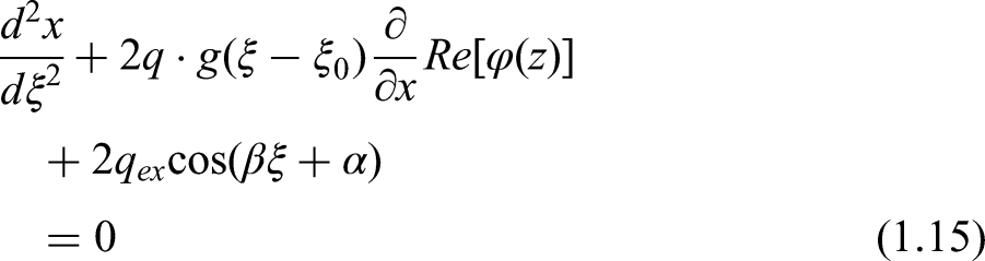
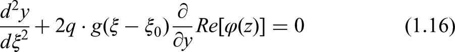
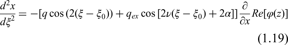
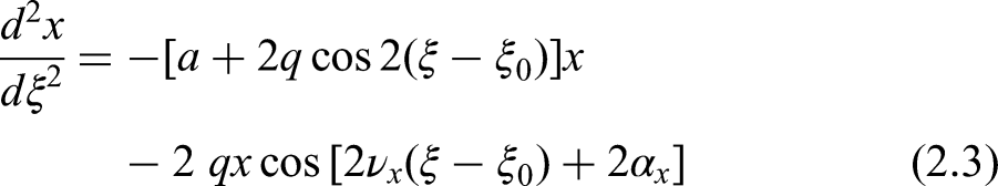
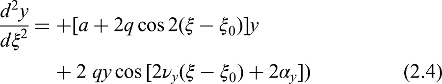
To study the QMF ion-optical properties with DE, a trajectory method based on numerical integration of the ion motion equations in a modified quadrupole field is used ⁵¹ :

$${\displaystyle \frac{d^{2}x}{d{\xi }^2}=-[a+2q\cos 2(\xi -{\xi }_0)]x-2qx\cos [2{\nu }_x(\xi -{\xi }_0)+2{\alpha }_x]}$$

(2.3)

$${\displaystyle \frac{d^{2}y}{d{\xi }^2}=+[a+2q\cos 2(\xi -{\xi }_0)]y+2qy\cos [2{\nu }_y(\xi -{\xi }_0)+2{\alpha }_y])}$$

(2.4)

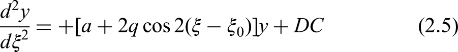
For zero frequency ${\nu }_y=0$ , the equation of motion along the $y$ coordinate is written in the following form ⁵⁵ :

$${\displaystyle \frac{d^{2}y}{d{\xi }^2}=+[a+2q\cos 2(\xi -{\xi }_0)]y+DC}$$

(2.5)

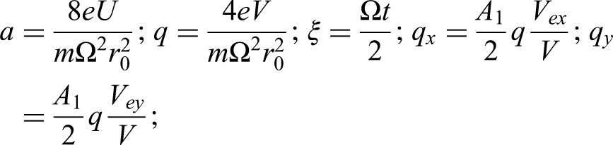
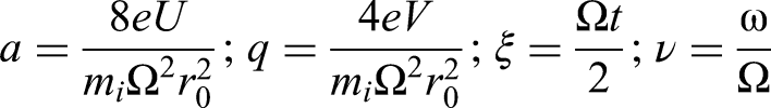
Here x and y are transverse coordinates normalized to the design parameter $r_0$ . The input dimensionless parameters in equations (3–5) are expressed through material parameters as follows:

$$a={\displaystyle \frac{8eU}{m{\mathrm{\Omega }}^2{r}_0^2};q={\displaystyle \frac{4eV}{m{\mathrm{\Omega }}^2{r}_0^2};\xi ={\displaystyle \frac{\mathrm{\Omega }t}{2};q_x={\displaystyle \frac{A_1}{2}q{\displaystyle \frac{V_{ex}}{V};q_y={\displaystyle \frac{A_1}{2}q{\displaystyle \frac{V_{ey}}{V};}}}}}}}$$

$$DC={\displaystyle \frac{4A_{1}e{U}_y}{m{\mathrm{\Omega }}^2{r}_0^2},{\nu }_x={\displaystyle \frac{{\omega }_x}{\mathrm{\Omega }},{\nu }_y={\displaystyle \frac{{\omega }_y}{\mathrm{\Omega }}}}}$$

(2.6)

where e and m are the charge and mass of the ion, U and V are the DC and AC amplitude of the quadrupole potentials $\pm (U+Vcos\mathrm{\Omega }t)$ , $r_0$ is the radius of the inscribed circle between the electrodes, a and q are parameters of the Mathieu equation, ${\xi }_0$ is the initial phase, $q_x$ and $q_y$ are dimensionless amplitudes of dipole potentials, and DC is the dimensionless potential applied to Y electrodes.

QMF transmission contour

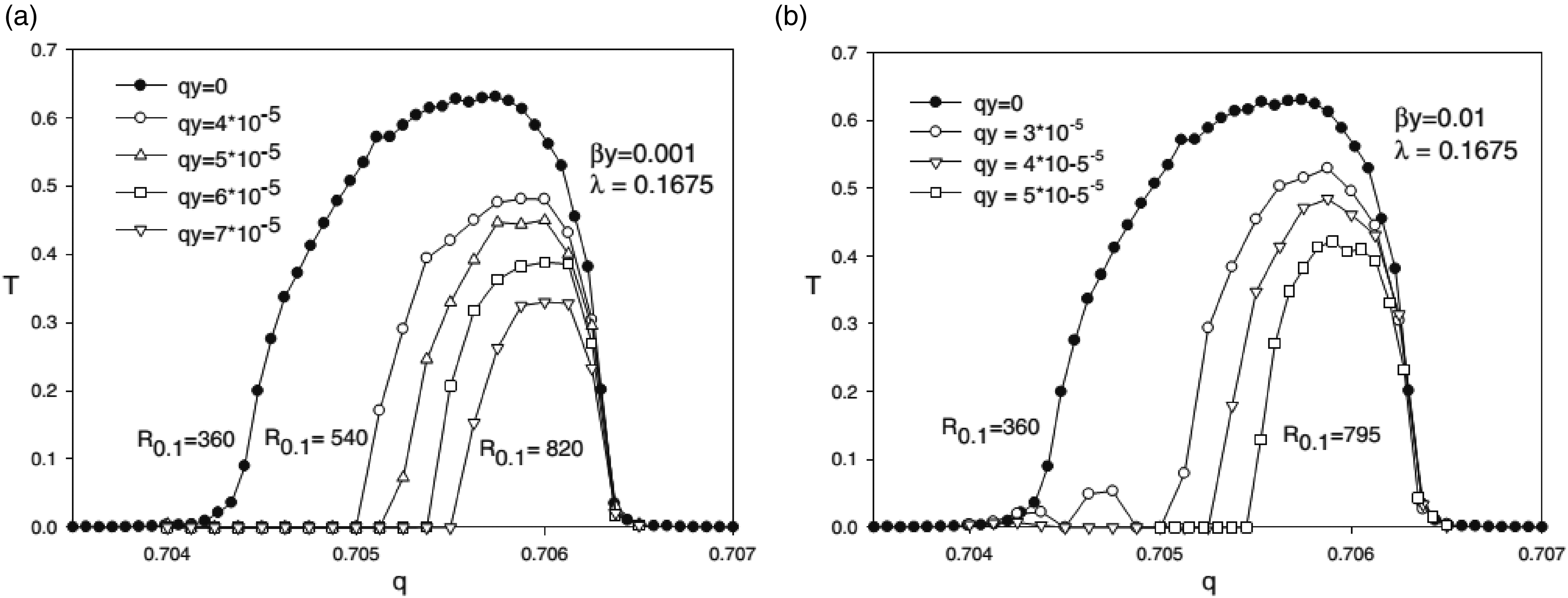
The effect of DE is illustrated in Figure 32 at the two frequencies ${\nu }_y=0.0005$ (a) and ${\nu }_y=0.005$ (b). In this case, the instability lines follow along the isolines ${\beta }_y=0.001$ and ${\beta }_y=0.01$ in the closest to the stability boundary ${\beta }_y=0$ . When increasing to frequency ${\nu }_y=0.005$ , harmful “tails” appear on the transmission contour, due to the fact that the instability band is separated from the border at small amplitudes $q_y$ . At the operating frequency $F=2\pi /\mathrm{\Omega }=1MHz$ , the excitation frequencies $f={\nu }_{y}F$ will be 0.5kHz and 5 kHz.

Figure 32.

Transmission contours of the QMF with dipole excitation of ions along the Y coordinate (a) at the frequency ${\nu }_y={\beta }_y/2=0.0005$ and (b) at the frequency ${\nu }_y=0.005$ at the indicated values of the amplitude $q_y$ . The scanning parameter $\lambda =0.1675$ . ⁵²

A study of QMF with circular electrodes and DE, characterized by the design parameter $r/r_0$ , revealed a slight advantage in analyzer transmission $r/r_0=1.109$ compared to $r/r_0=1.142$ , $1.130$ and $1.126$ . ⁵⁴

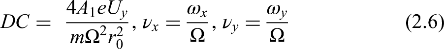
From Figure 33(a) shows that the resolving power reaches $R_{0.1}=2000$ at certain parameters $q_y=0.00003,{\nu }_y=0.001$ of DE in the case of an ideal quadrupole field. Compared to the usual way of changing the resolution by changing the scanning parameter λ, the use of DE doubles the resolution. The use of round rods (Figure 33(b)) leads to a decrease in the resolution approximately by a factor of two even in the case of DE. Hence, we can conclude that the use of DE with fixed parameters $q_y,{\nu }_y$ allows increasing the QMF transmission for a given value of resolution.

Figure 33.

Transmission-resolution curves for ideal field (a) and round rods (b); (a) 1—change in $\lambda$ ; 2—change in $\lambda$ and constant excitation parameters $q_y=0.00003,{\nu }_y=0.001$ ; 3—change in $\lambda$ and constants $q_y=0.00005,{\nu }_y=\mathrm{0.005.}$ (b) Round rods (r/ $r_0=1.130$ ), 1—without dipole excitation and 2—with dipole excitation $q_y=0.00005,{\nu }_y=0.005$ . ⁵⁴

Dipole excitation in the third stability region

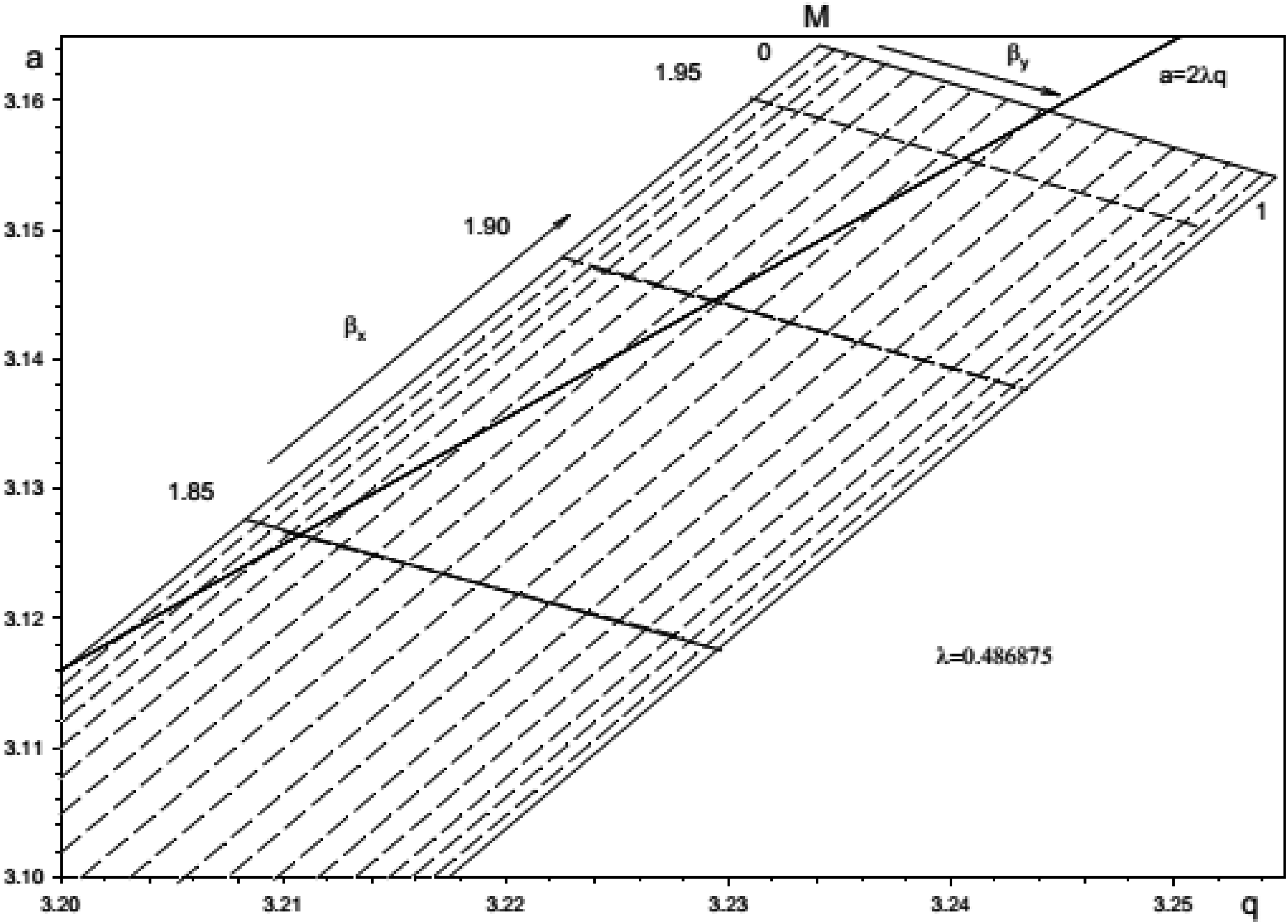
As the parameter λ increases, the scanning line approaches the tip M and the bandwidth $\mathrm{\Delta }q$ decrease and resolving power $R=q_M/\mathrm{\Delta }q$ increase (Figure 34). Thus, the separation of ions occurs when ${\beta }_y\to 0$ and ${\beta }_x\to 2$ . In this case, we can change the X and Y boundaries by DE at frequencies ${\nu }_x\approx 1$ and ${\nu }_y\approx 0$ . When constant potentials $\pm U_d$ are applied to the opposite Y electrodes, the case when the excitation frequency ${\nu }_y=0$ is realized. According to Figure 34, for dipolar excitation along the isolines ${\beta }_x=1.99$ and ${\beta }_y=0.01$ , the resonance frequencies ${\nu }_x={\nu }_y=0.005$ .

Figure 34.

The working tip M of the third stability area. The dotted lines are isolines ${\beta }_x$ and ${\beta }_y$ . The coordinates of the vertex M: $a_M=3.1643,q_M=\mathrm{3.2308.}a=2\lambda q$ is the scanning line ( $\lambda =0.4869$ ). ⁵²

In Figure 35 to compare the efficiency of the DE X and Y boundaries of the third stability region, the QMF transmission contours are shown. The effect of frequencies ${\nu }_y=0.005,0.995,1.005$ along the excitation line ${\beta }_y=0.01$ is shown in Figure 35а. The frequency ${\nu }_y=0.005$ corresponds to the basic harmonic of the ion oscillations with the frequency ${\nu }_y={\beta }_y/2$ , when the amplitude is maximal. The other resonance frequencies $0.995$ and $1.005$ are represented by the components of ion oscillations with frequencies ${\nu }_y=1-{\beta }_y/2$ and ${\nu }_y=1+{\beta }_y/2$ . One can see that the excitation intensity, characterized by the resolution $R_{0.1}$ , is strongest at the fundamental harmonic ${\nu }_y={\beta }_y/2$ with a small DE amplitude $q_y=0.0005$ . By increasing the amplitude $q_y$ , it is possible to effectively excite the resonance along the isoline ${\beta }_y=0.01$ at frequencies $0.995$ and $1.005$ close to the frequency of the RF generator. This considerably simplifies the problem of supplying Y electrodes.

Figure 35.

Transmission contours in the tip M during the excitation of isolines: (a) ${\beta }_y=0.01$ with amplitude $q_y=0.0005$ and frequencies ${\nu }_y=0.005,0.995,1.005$ ; (b) ${\beta }_x=1.99$ with amplitude $q_x=0.001$ and frequencies ${\nu }_x=1.005,0.995,0.005,1.995$ . The scanning parameter $\lambda =0.4885$ . The separation time $n=50RF$ periods. ⁵²

The effect on the right side of the transmission contour by DE at the X rods is illustrated in Figure 35(b). The possible resonance frequencies are ${\nu }_x=1.005,0.995,0.005,1.995$ . Excitation is most effective at frequencies ${\nu }_x=1.005,0.995$ , close to the main frequency. It is possible to use frequency ${\nu }_x=1.995$ with increased amplitude of dipole voltage $q_x$ . This is convenient for the technical realization of the dipole voltage on the X rods. Note that in the upper tip of the second region is achieved resolving power $R_{0.1}=390$ , determined by 10% of the peak height level, with a small sorting time $n=50$ periods of RF field and 45% of the transmittance level. Let's specify that amplitude $q_y$ =0.001 at amplitude $V=1000V$ of the RF oscillator corresponds to $V_y\cong (q_y/q)V=0.001/3.23\cdot 1000Volt=0.31Volt$ .

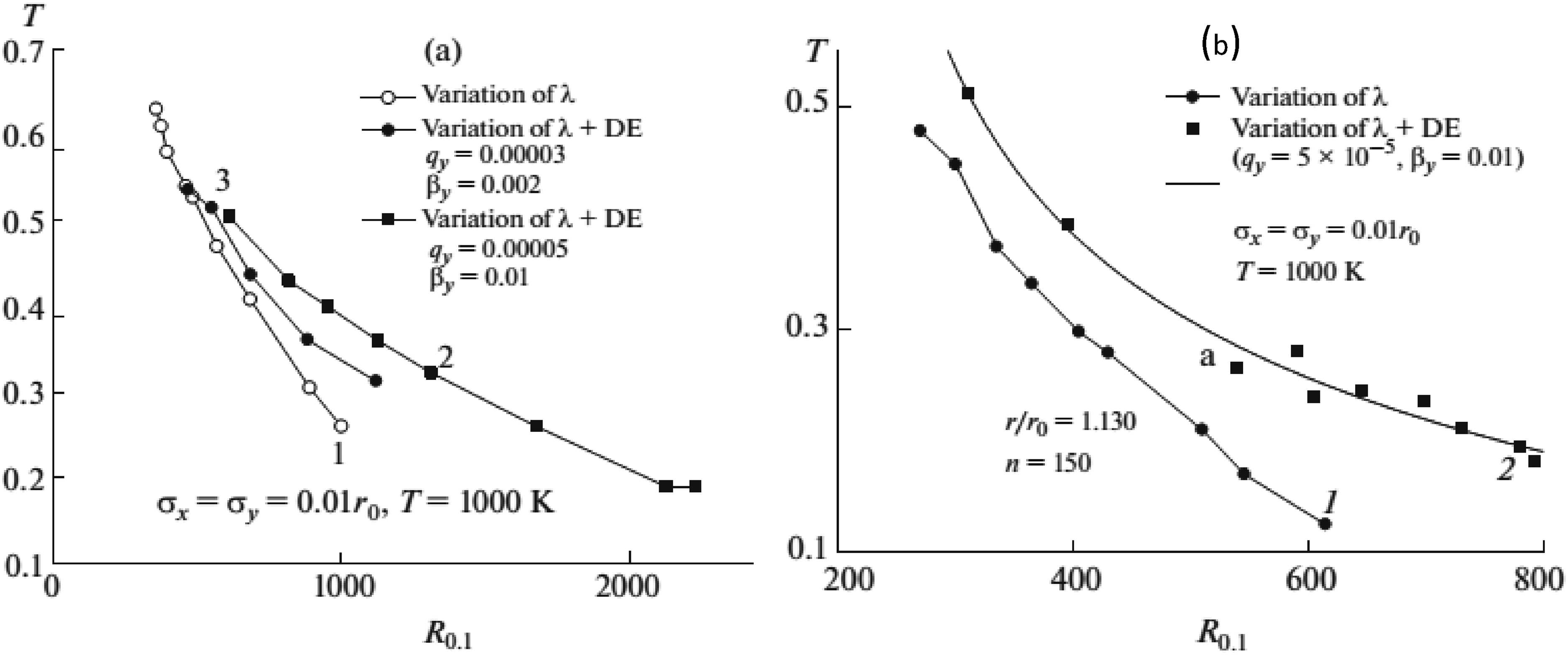
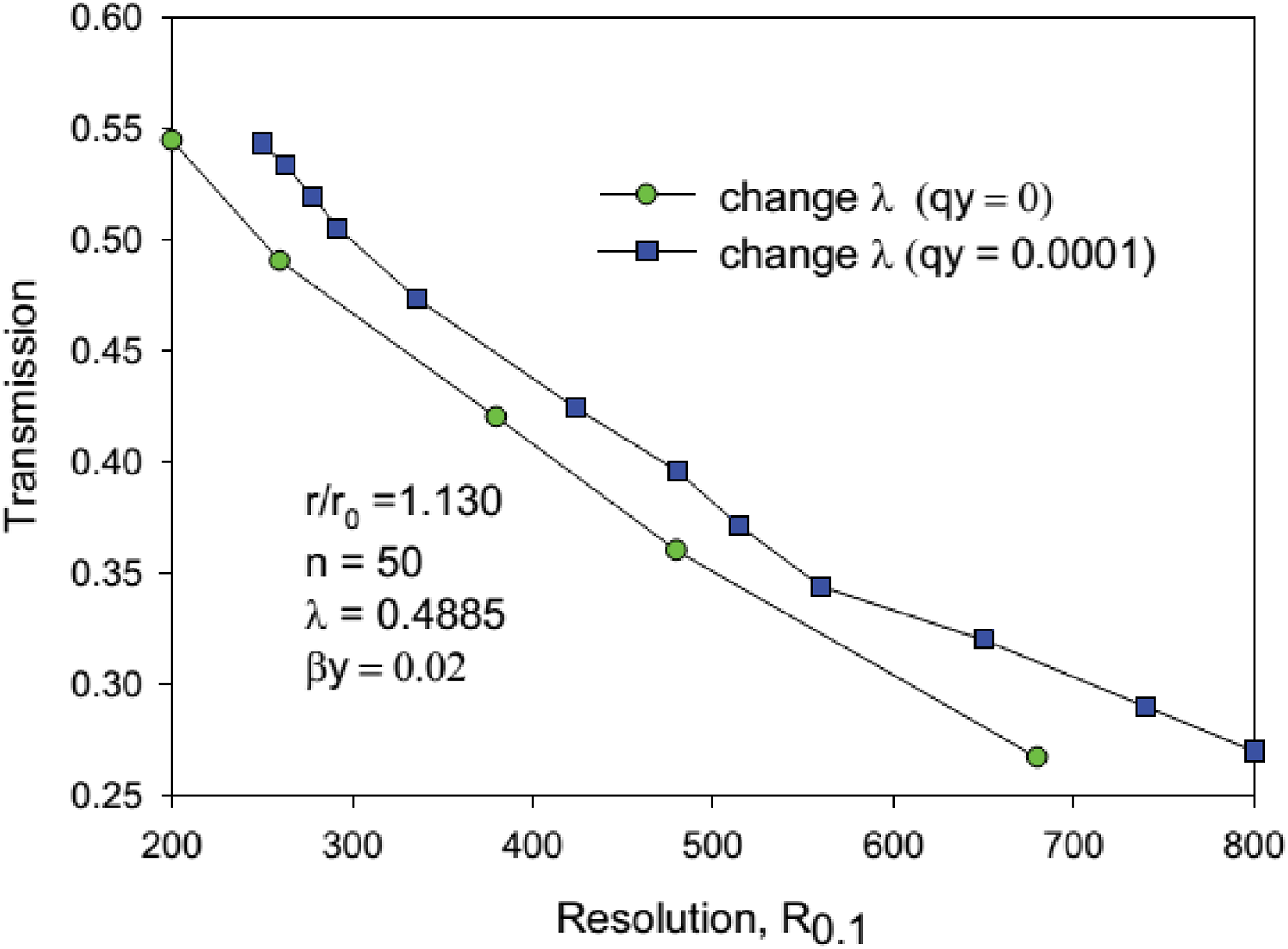
The effect of DE along the Y coordinate of the QMF with circular electrodes ( $r/r_0=1.130$ ) is shown in Figure 36. It can be seen that in the presence of constant excitation the mass transmission is higher than in the normal mode of operation of the QMF. The optimal shape of the transmission contour is achieved on the electrode structure with $r/r_0=1.130$ . DE gives a gain in QMF transmission of about 5–10% at a given resolution.

Figure 36.

Dependence of transmission coefficient T on resolving power $R_{0.1}$ for two ways of tuning QMF with round electrodes: by changing the scanning parameter $\lambda$ without dipole excitation $(q_y=0)$ or with constant dipole excitation with $q_y=0.0001$ and frequency ${\nu }_y=0.01$ . Round rods with $r/r_0=1.130$ . ⁵²

Dipolar excitation at frequencies ${\mathit{\nu }}_{\mathit{y}}=0$ and ${\mathit{\nu }}_{\mathit{x}}=1/2$

It turns out that it is possible to form a transmission loop at frequencies ${\nu }_x=0.5$ and ${\nu }_y=0$ corresponding to the boundary values ${\beta }_x=1$ and ${\beta }_x=0$ . ⁵⁵

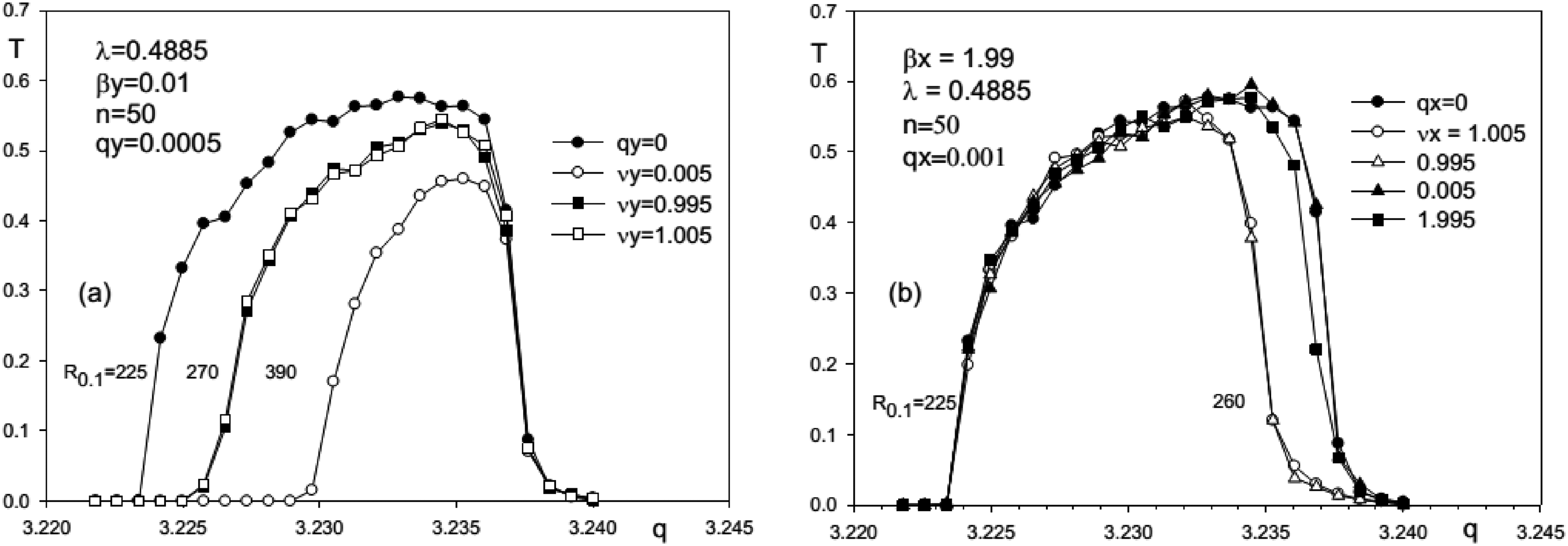
This is illustrated in Figure 37, which shows the transmittance contours for the specified values of the excitation amplitude $q_x$ . As the amplitude $q_x$ increases, the resolving power increases too and the QMF transmission decreases. The largest value of resolving power $R_{0.5}=5000$ is achieved at parameter $\lambda =0.1667$ (Figure 37(b)), when the initial resolution is maximal at $q_x=0$ . Note that at 30% transmittance, the resolving power is $R_{0.5}=3000$ (Figure 37(b)) and at the same transmittance $R_{0.5}=1400$ (Figure 37(a)). Thus, the use of DE at the frequency ${\nu }_x=0.5$ allows to double the resolving power at the same transmittance. However, a powerful low-mass “tail” is observed in this case.

Figure 37.

Transmission contours at two values of the parameter $\lambda$ : $0.166$ (a) and $0.1667$ (b). Dipole excitation at the frequency ${\nu }_x=0.5$ . ⁵⁵

The transmission contours at a constant auxiliary dipole $DC$ potential at the Y electrodes and the specified values of the amplitude $q_x$ and a constant value of $\lambda =0.167$ are shown in Figure 38(a). Increasing the amplitude $q_x$ removes the right side of the peak, resulting in its triangular shape. What is important here is that the tails of the peaks are eliminated when the ion separation time is $n=150$ periods. A resolution of $R_{0.5}=4900$ is achieved at a QMF transmittance of 20%. The simultaneous change of DC and AC potential $q_x$ results in a symmetrical peak shape without a “tail” (Figure 38(b)). A resolution of $R_{0.5}=10,000$ at 10% transmission level is achieved. The input ion beam with a Gaussian distribution at the QMF input aperture is described by the standard deviation ${\sigma }_x={\sigma }_y=0.01r_0$ .

Figure 38.

(a) The shape of the transmission circuit at the excitation combination at two frequencies ${\nu }_y=0$ and ${\nu }_x=0.5$ . (a) The potential $DC$ $=0.0002$ is constant and the resolution is changed by increasing the amplitude $q_x$ . (b) Simultaneous change of DC and $AC$ $q_x$ potentials. ⁵⁵

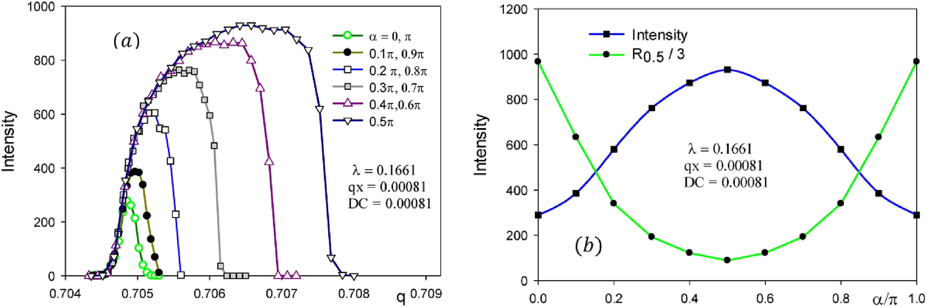
Figure 39 illustrates the effect of the phase shift α of the DC dipole potential $q_x=0.00081$ with frequency ${\nu }_x=0.5$ of the excitation circuit. When α changes from $0$ to $\pi /2$ , the right side of the peak shifts and the shape of the circuit becomes triangular (Figure 39(a)). Further, when $\alpha$ increases from $\pi /2$ to $\pi$ , the peak shifts to the left and restores its original shape. The change of the peak intensity and resolution with the phase shift $\alpha$ is shown in Figure 38(b). Intensity and resolution $R_{0.5}$ with change of $\alpha$ occurs in antiphase, when intensity is maximal, resolution is minimal. The periodicity of change of $R_{0.5}$ equals to $\pi$ , which corresponds to the period of the RF field.

Figure 39.

(a) Influence of phase shift α on the mass peak. (b) Dependences of peak intensity and resolution $R_{0.5}$ on phase shift $\alpha$ . ⁵⁵

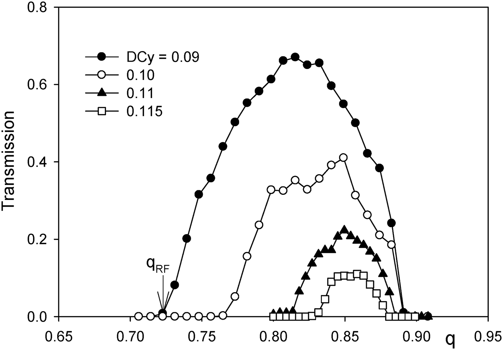
The effect of a constant DC potential on the X or Y electrodes in the absence of a $DC$ quadrupole voltage U, i.e. $a=0$ , is interesting. This mode of powering the QMF provides ion separation with a small resolving power (Figure 40). As the DC potential increases, the resolving power increases and the transmittance decreases. Such a mass filter can be used as a prefilter to remove large mass ions during operation in the second stability region.

Figure 40.

Transmission contours of a QMF operating in RF mode only with dipole potential DC =  $0.09,0.1,0.11$ and $0.115$ . Here $q_{RF}$ is the left boundary of the window transmission. ⁵³

X stability islands and dipole excitation

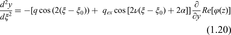
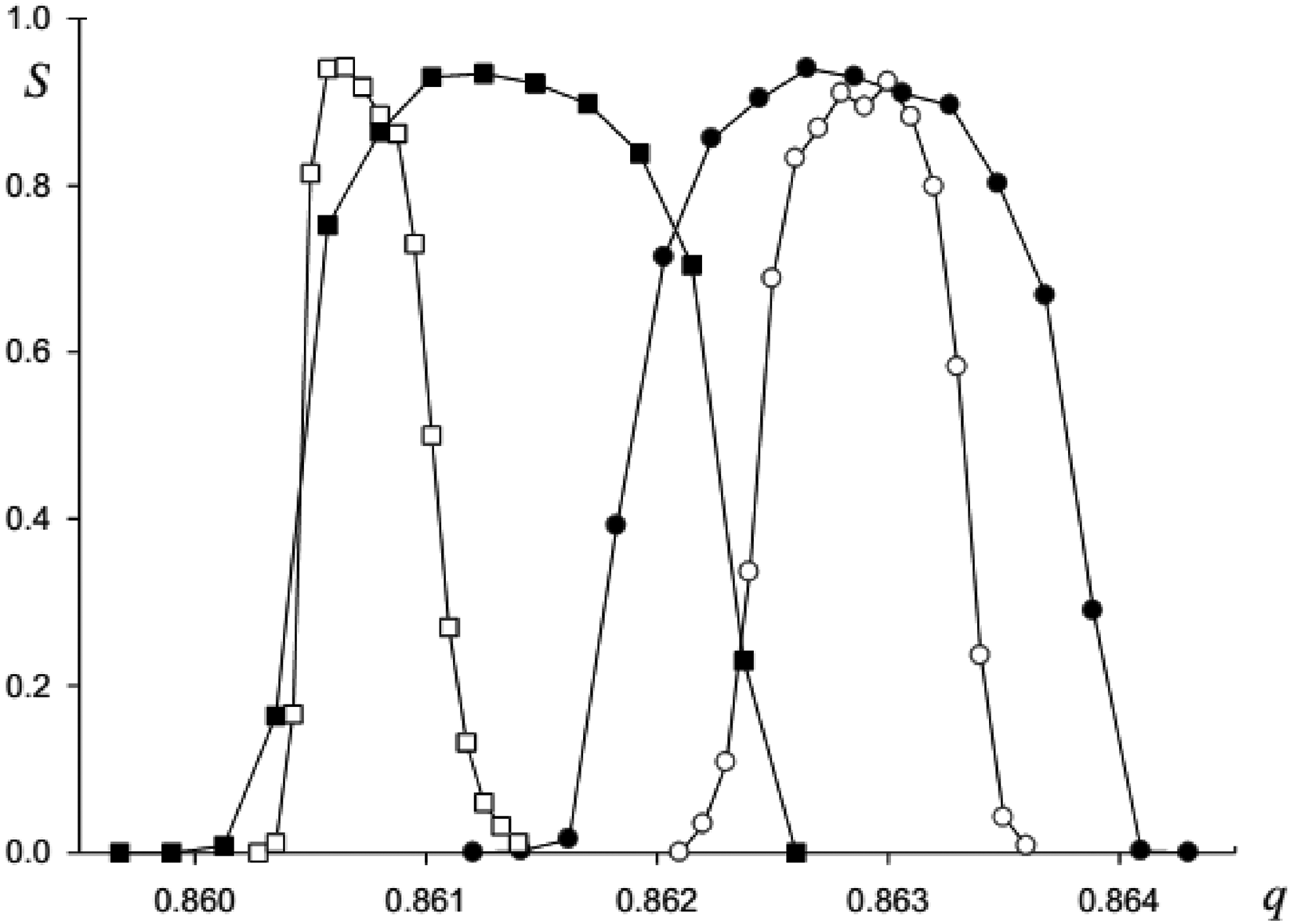
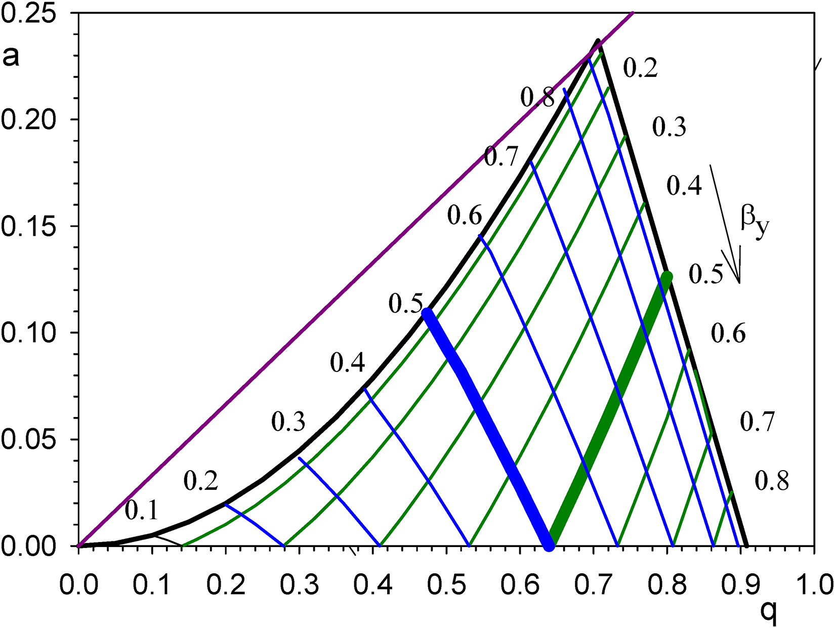
Figure 41(a) shows the stability islands created by an additional quadrupole RF voltage of amplitude $q_x=0.05$ and frequency $\nu =49/25$ . We distinguish the stability islands X1 and X2 following along the ${\beta }_x$ isoline, since the scanning line $a=2\lambda q$ crosses the X boundaries of the islands when the removal of the ions goes to the Y electrodes. As a result, this ensures that there are no significant “tails” of the mass peaks.

Figure 41.

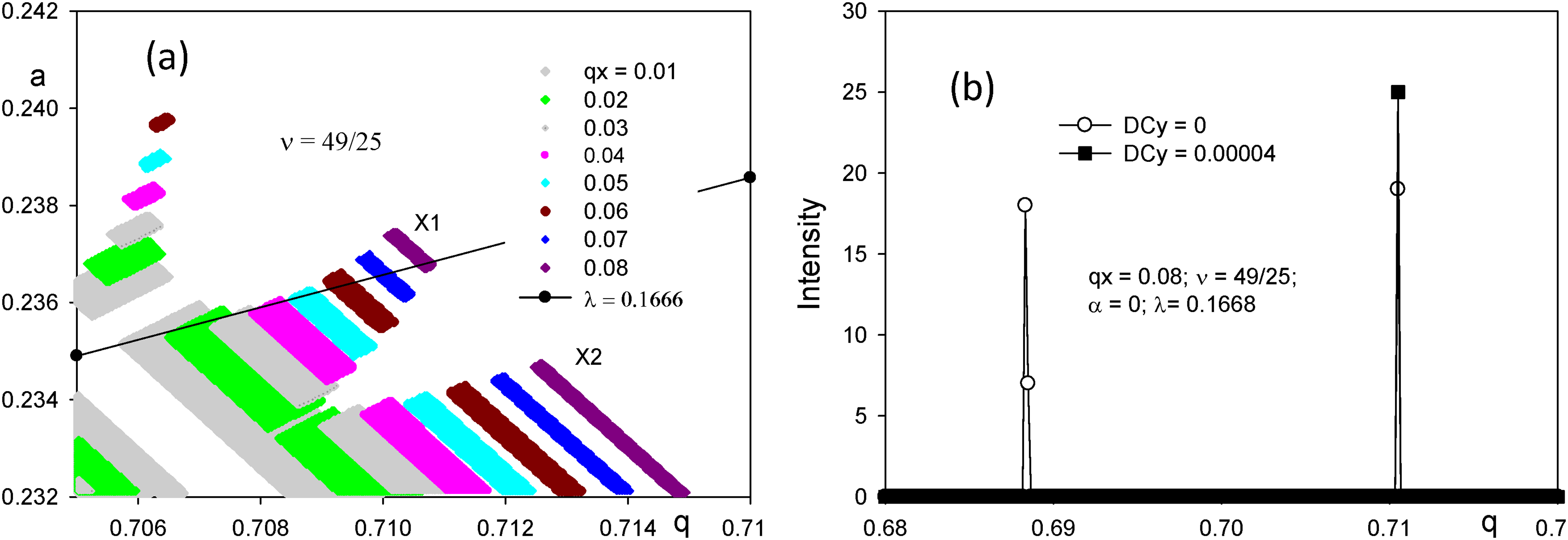
(a) Stability islands of X1 and X2 on the a and q parameter plane, initiated by a quadrupole additional voltage with amplitude $q_x=0.05$ and frequency $\nu =49/25$ . (b) transmission contours along the line scan $a=2\lambda q$ without $(D{C}_y=0)$ and in the presence of a dipole potential $DCy=0.0004$ . ⁵³

Operation in the stability islands X1 and X2 (Figure 41(a) is complicated by the fact that these islands are “shaded” by the stability bands following along the isolines ${\beta }_y$ . As a result, harmful peaks (Figure 41(b), $D{C}_y=0$ ) appear when the scanning line $a=2\lambda q$ crosses this Y stability band. These bands can be eliminated by an additional potential $D{C}_y=0.00004$ . Figure 41(b) shows the result of scanning over a wide range of parameter $q=0.68-0.72$ . The left peak ( $D{C}_y=0$ ) is due to the presence of a narrow ${\beta }_y$ stability band. When the $D{C}_y$ potential is added to the Y rods, the first peak disappears and the second one, corresponding to the transmittance of the X1 island, remains.

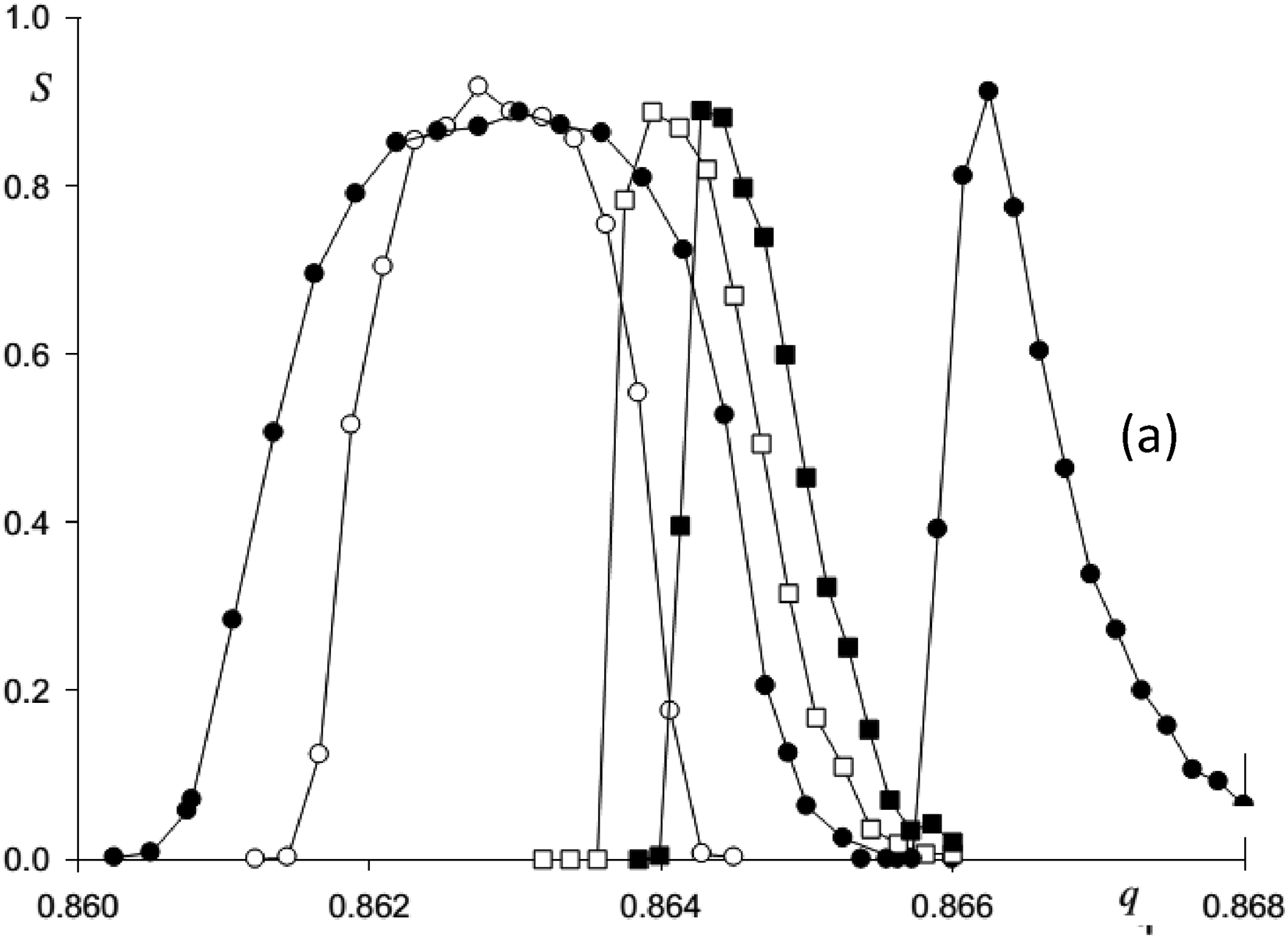
The transmission contours in the stability island X1 (Figure 41(a)) under quadrupole excitation with frequency $\nu =49/25$ are shown in Figure 42(a). As the amplitude $q_x$ increases, the peak shifts and the resolving power increases to $R_{0.5}\cong 4800$ . The results of the simulation of the transmission contour of the round rod QMF are shown in Figure 42(b) for three values of the design parameter $\frac{r}{r_0}=1.125,1.130$ and $1.145$ . As the $r/r_0$ value decreases, the peak shifts to the left along the q -axis, and the resolving intensity of the peaks is approximately the same. For an ideal quadrupole field, the transmission of the QMF is $1.5$ times greater. The frequency and amplitude of the quadrupole excitation are $\nu =1/36$ and $q_x=0.025$ , respectively.

Figure 42.

Transmission contours in stability islands: (a) $\nu =\frac{49}{25},q_x=0.06,0.07,0.08$ ; (b) transmission contours when using round electrodes in the island, defined by parameters: additional quadrupole voltage amplitude $q_x=0.025$ and frequency $\nu =1/36$ . ⁵³

Quadrupole mass filter with quadrupole excitation

Parametric resonance excitation

Parametric resonance is a phenomenon consisting in the oscillations amplitude increase when the parameters of the oscillating system periodically change.^58,59 If in the equations of ion motion the parameters $a,q$ change according to the harmonic law, it leads to parametric resonance. Devant first observed the phenomenon of parametric resonance excitation of ion oscillations under the application of an auxiliary RF field in 1989. ⁶⁰ Experimentally, such a phenomenon manifested itself in an improvement in the quality of the spectrum at relatively high masses when an auxiliary quadrupole RF voltage was applied. However, the physical nature of the phenomenon was not disclosed. Later Kozo^61,62 found that the auxiliary quadrupole voltage of small amplitude leads to the creation of an unstable band inside a stable band (literally “of unstable band generation inside a stable band”). Alfred, Londry, and March in 1993 developed the theory of first-order quadrupole parametric resonance excitation. ⁶³

Later, Sudakov et al. established frequencies of parametric resonance of order K. ⁶⁴ The point is that the parametric resonance takes place under the condition ⁵⁸ :

$$T=0.5K{T}_n,K=1,2,3,..,$$

(3.1)

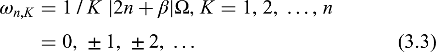
where $T=2\pi /\omega$ is the period of auxiliary RF voltage $\pm V^{\mathrm{\prime }}cos\omega t$ applied to the opposite pairs of QMF rods (Figure 9), $T_n$ is the period of free ion oscillations. Frequency of own ion oscillations is equal to

$${\omega }_n=|2n+\beta |{\displaystyle \frac{\mathrm{\Omega }}{2},n=0,\pm 1,\pm 2,\dots \mathrm{and}{T}_n={\displaystyle \frac{2\pi }{{\omega }_n}={\displaystyle \frac{4\pi }{|2n+\beta |\mathrm{\Omega }}}}}$$

(3.2)

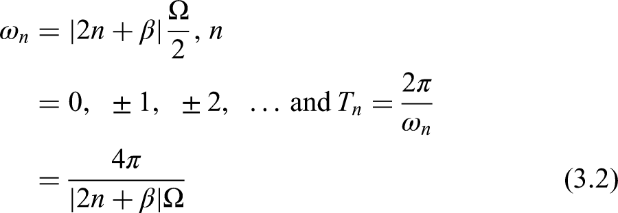
Substituting in equation (3.1) $T=2\pi /\omega$ and $T_n=4\pi /|2n+\beta |\mathrm{\Omega }$ we obtain that frequencies ${\omega }_{n,K}$ of parametric resonance of order K are equal ⁶⁴ :

$${\omega }_{n,K}=1/K|2n+\beta |\mathrm{\Omega },K=1,2,\dots ,n=0,\pm 1,\pm 2,\dots$$

(3.3)

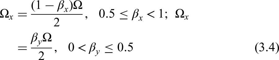
Thus, for the main temporal harmonic of ion oscillations $n=0$ , we find resonance frequencies ${\omega }_{0,1}=\beta \mathrm{\Omega },{\omega }_{0,2}=\beta \mathrm{\Omega }/2,{\omega }_{0.3}=\beta \mathrm{\Omega }/3,\dots$ . For first-order $K=1$ resonance: ${\omega }_{0,1}=\beta \mathrm{\Omega };{\omega }_{1,1}=(2+\beta )\mathrm{\Omega },{\omega }_{-2,1}=(2-\beta )\mathrm{\Omega },\dots$ . Let us express the frequencies of oscillations near the tip of the first stability region and consider the order of resonance K. Near the tip of the first stability region periodic motions have the following fundamental frequencies in the x and y directions

$${\mathrm{\Omega }}_x={\displaystyle \frac{(1-{\beta }_x)\mathrm{\Omega }}{2},0.5\le {\beta }_x<1;{\mathrm{\Omega }}_x={\displaystyle \frac{{\beta }_y\mathrm{\Omega }}{2},0<{\beta }_y\le 0.5}}$$

(3.4)

The conditions of the classical parametric resonance have the form ⁵⁸ :

$$K{\displaystyle \frac{2\pi }{\omega }=0.5{\displaystyle \frac{2\pi }{{\mathrm{\Omega }}_x};K{\displaystyle \frac{2\pi }{\omega }=0.5{\displaystyle \frac{2\pi }{{\mathrm{\Omega }}_y}}}}}$$

(3.5)

For the fundamental frequencies (3.4) of ion oscillations, condition (5.5) takes the form:

$$\nu =\omega /\mathrm{\Omega }=(1-{\beta }_x)/K={\beta }_y/K$$

(3.6)

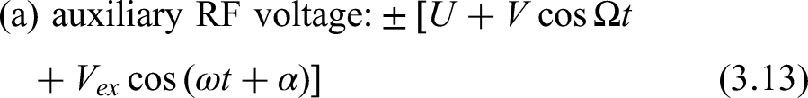
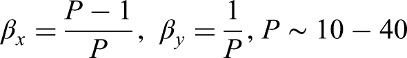
The number $K=1,2,3,\dots$ is the resonance order. As the order of K increases, the required amplitude of the auxiliary quadrupole voltage grows rapidly. Experimentally, Callings and Douglas observed high-order instability bands. ⁶⁵ Parametric resonance can be realized by harmonic changes in one of the ion motion parameters: (a) using an auxiliary RF quadrupole voltage, (b) by amplitude modulation of the RF voltage, or (c) frequency or phase modulation.

Ion motion equations for resonant excitation

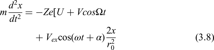
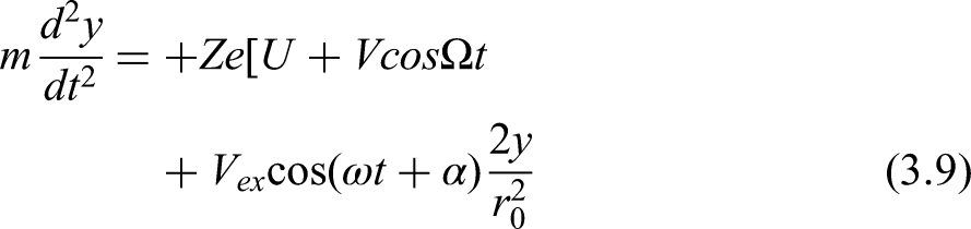
The potential distribution $\mathrm{\Phi }(x,y,t)$ in this case auxiliary excitation is of the form:

$$\mathrm{\Phi }(x,y,t)=[U+Vcos\mathrm{\Omega }t+{\mathrm{V}}_{\mathrm{ex}}\cos (\omega t+\alpha )](x^2-y^2)/(r_0^2)$$

(3.7)

According to Newton's second law, the equations of ion motion are

$$m{\displaystyle \frac{d^{2}x}{d{t}^2}=-Ze[U+Vcos\mathrm{\Omega }t+V_{ex}\cos (\omega t+\alpha ){\displaystyle \frac{2x}{r_0^2}}}$$

(3.8)

$$m{\displaystyle \frac{d^{2}y}{d{t}^2}=+Ze[U+Vcos\mathrm{\Omega }t+V_{ex}\cos (\omega t+\alpha ){\displaystyle \frac{2y}{r_0^2}}}$$

(3.9)

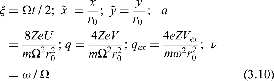
Let's introduce dimensionless parameters

$$\xi =\mathrm{\Omega }t/2;\tilde{x}={\displaystyle \frac{x}{r_0};\tilde{y}={\displaystyle \frac{y}{r_0};a={\displaystyle \frac{8ZeU}{m{\mathrm{\Omega }}^2{r}_0^2};q={\displaystyle \frac{4ZeV}{m{\mathrm{\Omega }}^2{r}_0^2};q_{ex}={\displaystyle \frac{4eZ{V}_{ex}}{m{\omega }^2{r}_0^2};\nu =\omega /\mathrm{\Omega }}}}}}$$

(3.10)

where $\xi$ is dimensionless time, $\tilde{x}$ and $\tilde{y}$ are dimensionless transverse coordinates.

After the change of variables, we obtain:

$$\begin{array}{r}{\displaystyle \frac{d^2\tilde{x}}{d{t}^2}+[a+2qcos(2(\xi -{\xi }_0))+2q_{ex}\cos (2\nu \xi +2\alpha )]\tilde{x}=0}\end{array}$$

(3.11)

$$\begin{array}{r}{\displaystyle \frac{d^2\tilde{y}}{d{t}^2}-[a+2qcos(2(\xi -{\xi }_0))+2q_{ex}\cos (2\nu \xi +2\alpha )]\tilde{y}=0}\end{array}$$

(3.12)

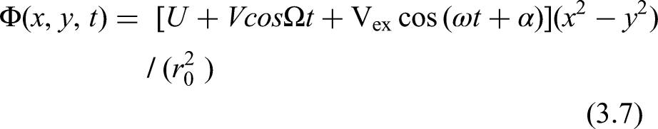
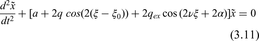
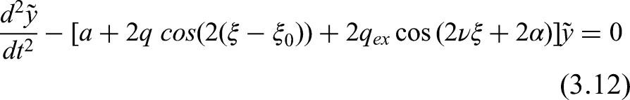
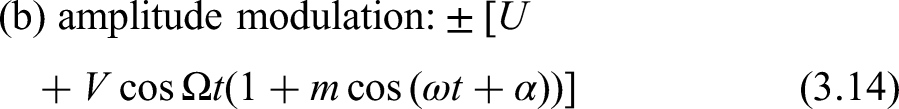
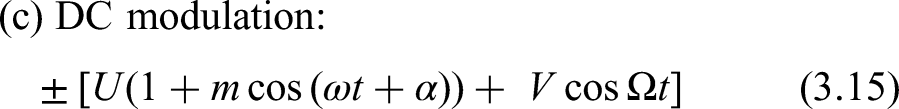
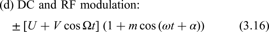
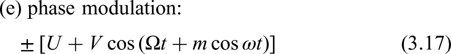
The ion motion equations (3.11) and (3.12) include the following parameters: DC potential U, amplitude of alternating voltage V, and frequency Ω. Consequently, changes of the above parameters according to the law sin or cos at the previously mentioned frequencies should lead to parametric resonance excitation of ion oscillations. Technically, this can be achieved by using ⁶⁶ :

$$(\mathrm{a})\mathrm{auxiliary}\mathrm{RF}\mathrm{voltage}:\pm [U+V\cos \mathrm{\Omega }t+V_{ex}\cos (\omega t+\alpha )]$$

(3.13)

$$(\mathrm{b})\mathrm{amplitude}\mathrm{modulation}:\pm [U+V\cos \mathrm{\Omega }t(1+m\cos (\omega t+\alpha ))]$$

(3.14)

$$(\mathrm{c})\mathrm{DC}\mathrm{modulation}:\pm [U(1+m\cos (\omega t+\alpha ))+V\cos \mathrm{\Omega }t]$$

(3.15)

$$(\mathrm{d})\mathrm{DC}\mathrm{and}\mathrm{RF}\mathrm{modulation}:\pm [U+V\cos \mathrm{\Omega }t](1+m\cos (\omega t+\alpha ))$$

(3.16)

$$(\mathrm{e})\mathrm{phase}\mathrm{modulation}:\pm [U+V\cos (\mathrm{\Omega }t+m\cos \omega t)]$$

(3.17)

$$(\mathrm{f})\mathrm{frequency}\mathrm{modulation}:\pm [U+V\cos (\mathrm{\Omega }t(1+m\cos \omega t))]$$

(3.18)

Stability islands

According to formula (3.6) for the excitation frequency $\nu =k/P,k<P$ and $k,P$ are integers, then the values ${\beta }_y=k/P$ and ${\beta }_x=1-k/P$ correspond to periodic oscillations of ions along X and Y coordinates. Because of resonance, instability bands following along the isolines ${\beta }_y=1/P,2/P,\dots ,(k-1)/P$ and ${\beta }_x=1-k/P,k=1,2,\dots ,(k-1)/P$ appear. The intensity (width) of the bands increases nonlinearly with the excitation amplitude $q_{ex}$ . These instability bands create stability islands, which are shown in Figure 43.

Figure 43.

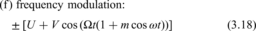
(a) Stability islands A, B and C observed in the experiment. RF oscillator frequency is 2.5 MHz, $\nu =$ 2.25 MHz is the resonant excitation frequency ⁶⁷ ; (b) calculated numerically modified stability diagram under the same conditions as in Figure 42(a): $\nu =\frac{9}{10},q_{ex}=0.012$ .

The experimental proof of the stability diagram splitting into islands during quadrupole excitation of ion oscillations is presented in. ⁶⁷ Ions with different charge-to-mass ratios arranged along the scanning line $a=2\lambda q$ (Figure 43). The value of $\lambda$ determines the slope at which the line crosses the tip of the Mathieu diagram and the range of $m/z$ ions that are stable. In the case of auxiliary quadrupole excitation, only the tip island A or two islands B and C or three islands A, B, and C can be crossed, depending on $\lambda$ and the excitation parameter $q_{ex}$ . As a result, single, double, or triple overlapping spectra can be observed (Figure 43(b)). It was found that the best resolution and isotopic sensitivity is achieved in island C. However, island B “shadows” island C, because the scan line passes both island B and island C at the same time. The straight lines show the boundaries of the unperturbed stability region. An increase in the amplitude of $q_x$ leads to a shift of the external islands outside the original stability region.

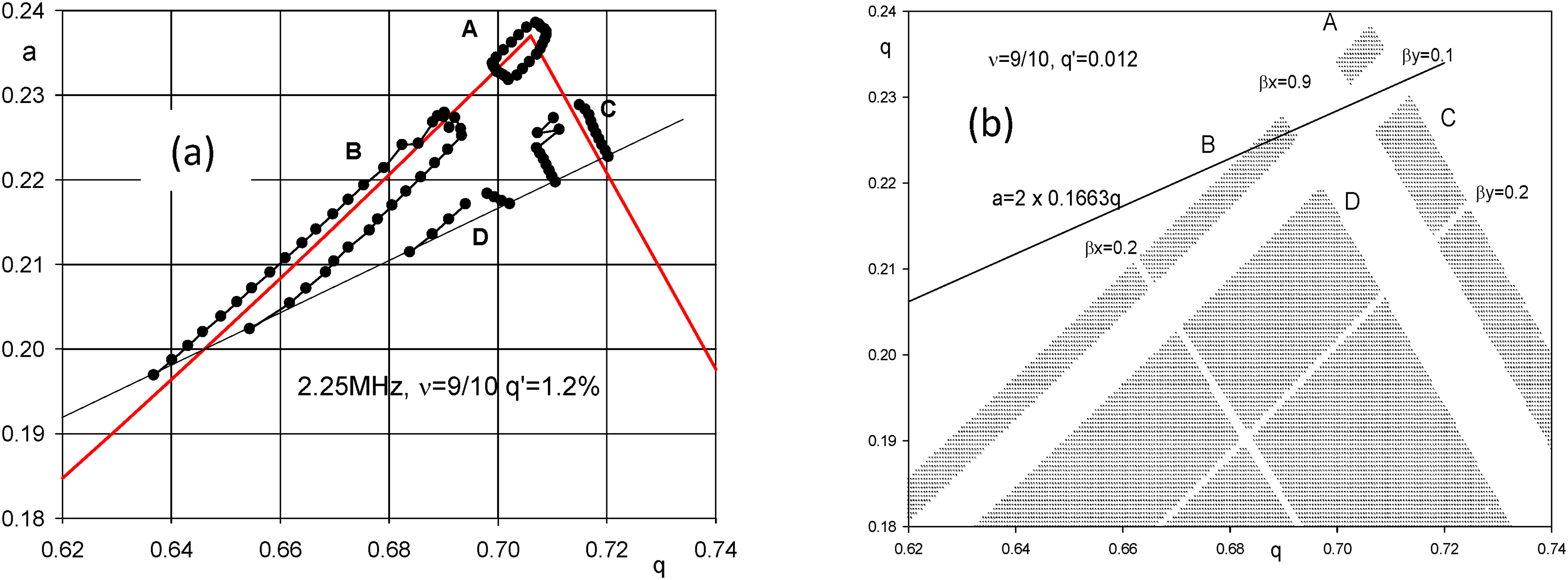
Figure 43(a) shows the stability islands formed by the instability bands following along the isolines ${\beta }_x=9/10,8/10,7/10,\dots ,1/10$ and ${\beta }_y=1/10,2/10,3/10,\dots ,9/10$ of the unperturbed stability zone. The most intense instability bands follow along the isolines ${\beta }_x=9/10$ and ${\beta }_y=1/10$ , cutting off the upper working stability island. The operation of the mass filter is possible in the upper and lower tips of the stability island, when it is possible to adjust the resolving power by changing the slope of the scanning line $a=2\lambda q$ . Figure 43(b) shows islands A, B, C, and D, the positions of which were experimentally determined on the $a,q$ plane. One can see an excellent agreement between theory (a) and experiment (b). In principle, it is possible to operate in other islands, such as island B, but in this case, an additional filter is needed to remove ions entering the spectrum through island C, in the case where the scanning line crosses two islands. This situation is illustrated in Figure 44, which shows the mass spectrum obtained in the stability islands B and C.

Figure 44.

Mass spectrum of ⁸⁰Ar²⁺ and isotopes obtained by scanning through two islands B and C at $q_{ex}=3.6\text{\%}.$ The ion energy is 5 eV, $\omega =9/10\mathrm{\Omega }=2.25MHz$ , $V_{ex}$ = 64 V, and $V=1254V(p-p)$ . ⁶⁷

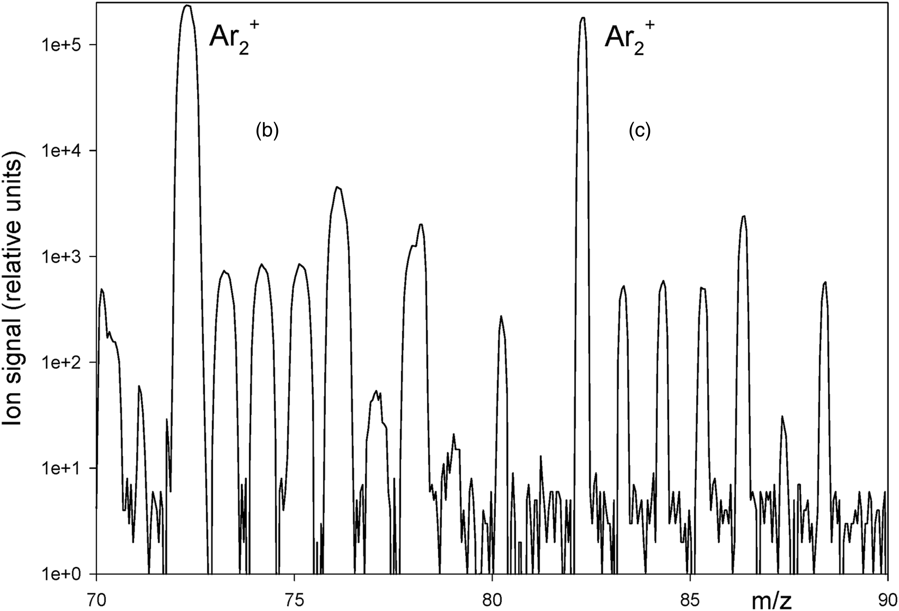
The $R{h}^{+}$ peak is shown in Figure 45 in the presence of quadrupole excitation and during normal operation. The presence of a low-mass “tail” of the transmission loop without excitation limits the isotopic sensitivity to a value of the order of ${10}^6$ . Operation in the stability island A at the tip eliminates the “tail” and allows isotopic sensitivity up to ${10}^8$ . ⁶⁷ This is the main advantage of QMF operation in the stability island.

Figure 45.

Mass peak of the rhodium $R{h}^{+}$ with excitation (black dots) and without excitation. ⁶⁷

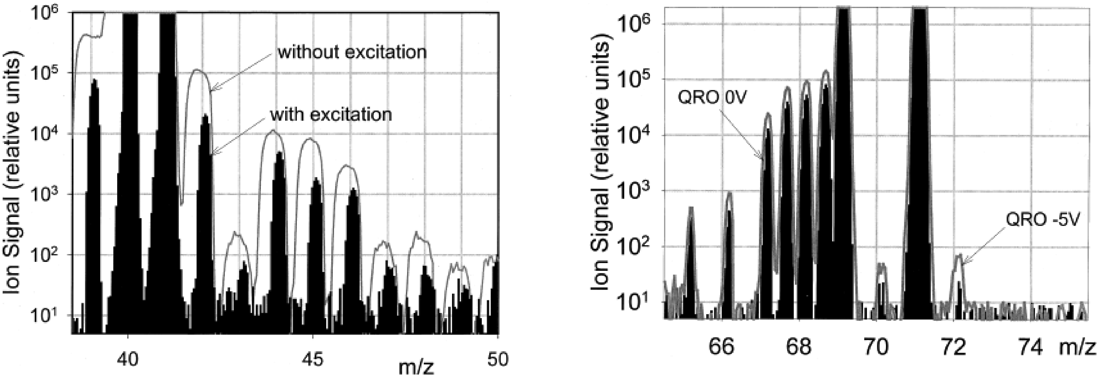
Figure 46 shows that operation in island A increases the resolving power and isotopic sensitivity at the expense of the loss in mass filter transmission. The data were obtained on a mass spectrometer with an inductively coupled plasma ion source.

Figure 46.

Mass spectrum sections: (a) without excitation and with excitation; (b) effect of changing the QRO potential of the Brubaker prefilter on the intensity of the peaks. ⁶⁷

The operation mode of the mass filter at the upper island has found practical applications in the creation of a quadrupole mass spectrometer for space research. ⁶⁸ The island parameters are excitation frequency $\nu =1.9167$ and amplitude $q_{ex}\approx 0.15$ .^68,69 In those papers, the separation mode in the upper stability island of the quadrupole mass filter with circular ( $r_0$  = 6.7 mm) and hyperbolic electrodes ( $r_0$  = 5.08 mm) is studied experimentally. The island was created by using an additional quadrupole RF voltage with relative frequency $\nu =2-{\beta }_y=\omega /\mathrm{\Omega }=1.9167$ , where $\mathrm{\Omega }/2\pi =1.06$ MHz and $1.4$ MHz are working frequencies of analyzers with circular or hyperbolic electrodes. A twofold increase in resolution $R_{0.01}$ was obtained for the QMF with circular electrodes. No increase in resolving power was observed for QMF with hyperbolic electrodes but the stability and reproducibility of mass isotope ratios of $K{r}^{+}$ peaks was increased by almost one order of magnitude. The quadrupole tank circuit for spaceborne MS was described ⁶⁹ in detail. The excitation frequency $\nu \approx 2$ was chosen in order to separate the frequencies of the RF oscillator and the additional quadrupole RF potential.

Calculation of the stability islands

The matrix method for calculating the ion trajectories in the quadrupole electric field is outlined in the book. ³⁶ Later this method was applied by M. Sudakov et al. ⁶⁴ for the case of the Hill equation, which describes the motion of ions with quadrupole resonance excitation (Eq. 3.11 and 3.12). If the dimensionless frequency $\nu$ of quadrupole excitation is represented as a simple irreducible fraction $\nu =\beta =k/P,k<P,k$ , and P are integers, then the ion trajectories are periodic with a period $2\pi P$ . ⁷⁰ On the other hand, functions $\cos (2(\xi -{\xi }_0))$ and $\cos (2\nu \xi +2\alpha )$ ) have a common period $\pi P.$ The stability condition is defined for the period $\pi P$ as in the case of the Mathieu equation for the period $\pi$ . ⁷⁰

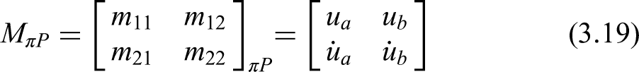
The stability condition is determined by the matrix $M_{\pi P}$ transform over the period $\pi P$ of the initial orthogonal coordinates and velocities: (a) $u_0=0$ , $u_0^{\mathrm{\prime }}=1$ и (b) $u_0=0$ , $u_0^{\mathrm{\prime }}=1$ ^68,71

$$M_{\pi P}={\left[\begin{array}{cc}{m}_{11}& m_{12}\\ m_{21}& m_{22}\end{array}\right]}_{\pi P}=\left[\begin{array}{cc}{u}_a& u_b\\ {\dot{u}}_a& {\dot{u}}_b\end{array}\right]$$

(3.19)

$m_{11}$ is the ion coordinate through period $P\pi$ under initial conditions (a), $m_{12}$ is the ion coordinate through period $P\pi$ under initial conditions (b), $m_{21}$ is the ion velocity through period $P\pi$ under initial conditions (a), and $m_{22}$ is the ion velocity through period $P\pi$ under initial conditions (b). Here $u=x$ or $u=y$ . The elements $m_{11}$ and $m_{22}$ can be calculated by any suitable numerical method of integration of ion motion equations (3.11) and (3.12) on the interval $0-\pi P$ . If the trace of the transform matrix $|m_{11}(a,q)+m_{22}(a,q)|=2$ , then the point $(a,q)$ corresponds to the boundary of the stability island. If $|m_{11}(a,q)+m_{22}(a,q)|>2$ , the ion trajectory is unstable (the amplitude of oscillations grows exponentially) and if $|m_{11}(a,q)+m_{22}(a,q)|<2$ , the point ( $a,q$ ) belongs to the stability island. The $M_{\pi P}$ matrix determines all ion-optical properties of the quadrupole field with resonant excitation. Thus, the parameter $\beta$ , which determines the ion oscillation spectrum, is expressed via the matrix elements as

$$2\cos (P\pi \beta )=m_{11}+m_{22}$$

(3.20)

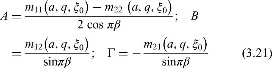
The values of the parameters of the capture ellipses A, B, and Г are^72,73

$$A={\displaystyle \frac{m_{11}\left(a,q,{\xi }_0\right)-m_{22}\left(a,q,{\xi }_0\right)}{2\cos \pi \beta };B={\displaystyle \frac{m_{12}\left(a,q,{\xi }_0\right)}{\sin \pi \beta };\mathrm{\Gamma }=-{\displaystyle \frac{m_{21}\left(a,q,{\xi }_0\right)}{\sin \pi \beta }}}}$$

(3.21)

The method for numerically calculating the position of the stability islands is as follows. A window on $a,q$ plane is set with parameters $a_{\min },a_{\max }$ and $q_{\min }$ , $q_{\max }$ . The step $\mathrm{\Delta }a=(a_{\max }-a_{\min })/N$ of scanning by the a coordinate and the step $\mathrm{\Delta }q=(q_{\max }-q_{\min })/N$ by the q coordinate are determined. At the nodes of this grid ( $a_i,q_j$ ), the equations of motion on the interval ( $0,\pi P$ ) are numerically integrated with initial conditions $u_0=0$ , $u_0^{\mathrm{\prime }}=1$ and $u_0=0$ , $u_0^{\mathrm{\prime }}=1$ . If stability conditions for x and y directions are simultaneously satisfied at point ( $a_i,q_j$ ), the pair ( $a_i,q_j$ ) of coordinates is memorized. The grid scan results in a two-dimensional array of ( $a_i,q_j$ ) stable coordinates. The accuracy of localization of the stability islands depends on the number N (enough 100–200) and the area of the scanning window.

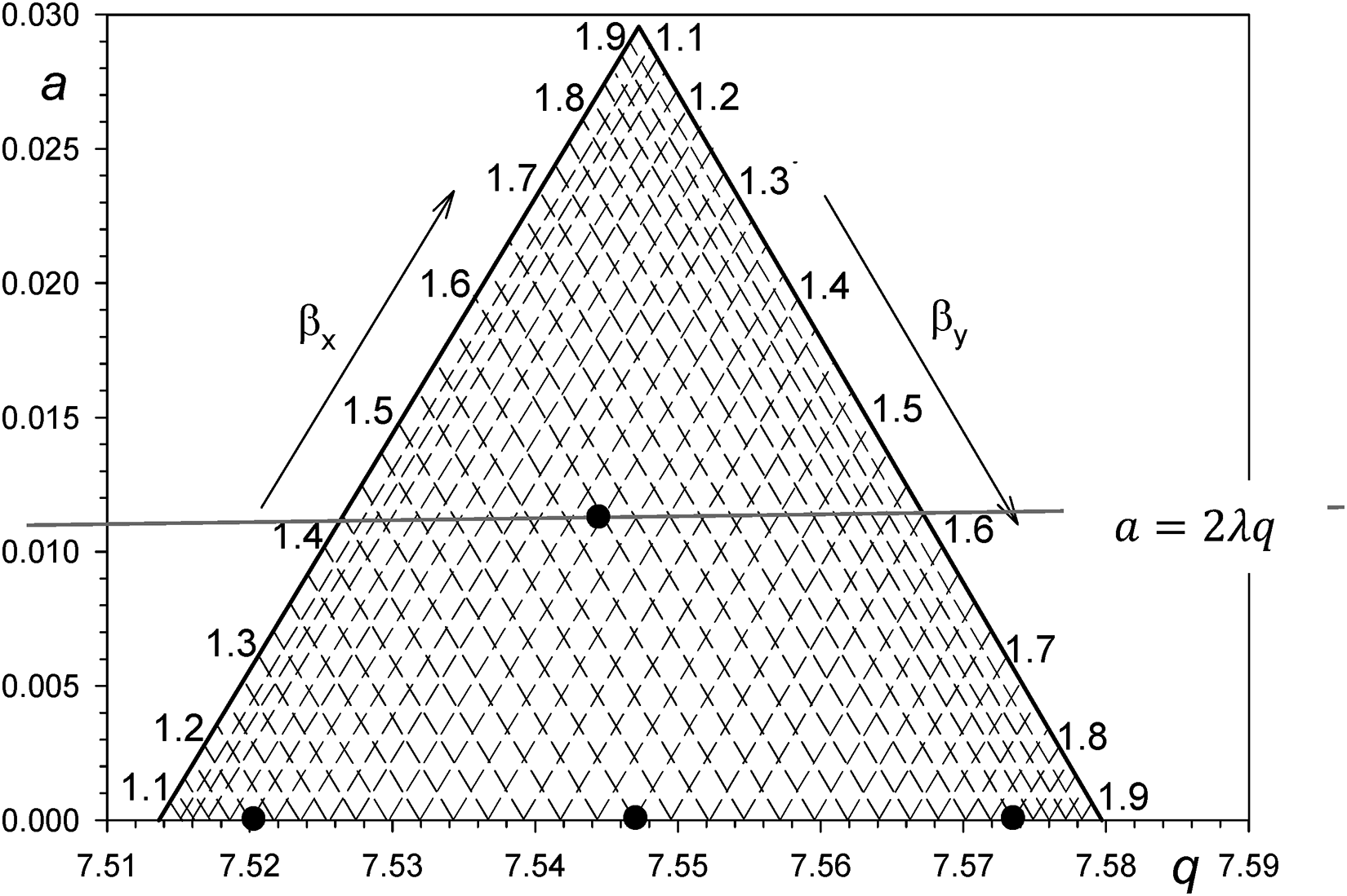
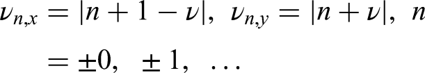
Stability islands (Figure 47) are defined by two parameters: the amplitude $q_{ex}$ and the excitation frequency ν. For practical applications, there are possible frequencies ν suitable for creating the upper working island of stability: $\nu =\beta ,1\pm \beta ;2\pm \beta ;3\pm \beta ;\beta =1/P;P=10-30$ , i.e. for frequencies $n=0,1,2,\mathrm{and}3$ from the frequency spectrum of ion oscillations ${\nu }_n=|n+\beta /2|$ . At $n>3$ , the harmonic amplitude drops rapidly. For $\nu =9/10$ , the main instability bands following along the isolines ${\beta }_x=1/20$ and ${\beta }_y=1/20$ , and correspond to excitation at frequencies ${\nu }_1=1\pm 1/20$ . Excitation at frequencies $2\pm \beta$ corresponds to the frequencies of natural ion oscillations ${\nu }_2=2\pm 1/P$ . In this case, there is a complex pattern of splitting of the stability region into islands. As the excitation amplitude $q_{ex}$ increases, the island shifts along the q -axis and the a -axis, its area decreases, and its shape is preserved (Figure 47(b)). As follows from the experiment, ⁶⁷ the shape of the island changes smoothly without jumps as the frequency ν and the amplitude $q_x$ change. The frequencies $\nu$ are chosen in the form of an irreducible simple fraction from the theoretical considerations mentioned above.

Figure 47.

(a) Stability islands at different orders of resonance $n=1(\nu =9/10,1.1),n=2(\nu =1/9,2.1),n=2(\nu =191/100)$ . (b) Effect of the excitation amplitude $q^{\mathrm{\prime }}$ ( $or{q}_{ex}$ ) on the position of the stability island with frequency $\nu =2-9/100=191/100$ .

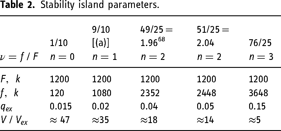
Figure 47 shows the upper working islands when the resonant frequencies ν increase with order of resonance n. Table 2 shows the values of resonant frequencies f for the operating frequency $F=1.2$ MHz and the ratio $V/V_{ex}$ of the required RF main voltage amplitudes to the auxiliary voltage. It can be seen that increasing the resonance frequency $f=\omega /2\pi$ leads to increasing the amplitude $V_{ex}$ . In the experiment,^68,69 the frequency $\nu =9/10$ was chosen from considerations that the resonance frequency $f=2.25\mathrm{MHz}$ would be close to $F=2.5\mathrm{MHz}$ in order to pass the additional signal through the main RF voltage amplifier path.

Table 2.

Stability island parameters.

$\nu =f/F$	1/10 $n=0$	9/10 [(a)] $n=1$	49/25 = 1.96 68 $n=2$	51/25 = 2.04 $n=2$	76/25 $n=3$
$F,k$	1200	1200	1200	1200	1200
$f,k$	120	1080	2352	2448	3648
$q_{ex}$	0.015	0.02	0.04	0.05	0.15
$V/V_{ex}$	$\approx$ 47	$\approx$ 35	$\approx$ 18	$\approx$ 14	$\approx$ 5

During the creation of the quadrupole mass spectrometer^54,69 for cosmic studies, the frequency $\nu$ was used close to the frequency $\nu =49/25$ (main drive frequency, MHz: $1.40,1.06$ ); (excitation frequency, MHz: 2 $.6834\mathrm{and}2.0317$ , ${\nu }_1=2.6834/1.40=1.9167$ $(r_0=5.08\mathrm{mm})$ and ${\nu }_2=2.0317/1.06=1.917$ ( $r_0=6.7\mathrm{mm}$ ). The excitation frequency is chosen for the purpose of frequency diversity and the use of a dual resonant single circuit. The calculation of the two-frequency resonant circuit is presented in. ⁶⁸

D. Douglas ⁷⁴ experimentally studied the operation of the mass filter with circular electrodes in the upper stability island in the presence of an octupole harmonic. The positions of stability islands A, B, and C in the presence of a 2%, 2.6%, and 4% octupole component were determined. In detail, the working upper stability island shown in Figure 48(a) was determined experimentally in. ⁷⁴ In the presence of 2–4% octupole component, the position of the stability island depends on the sign of a. The voltage $U>0$ at the X electrodes (the usual mode in the analysis of positive ions) corresponds to $a>0$ .

Figure 48.

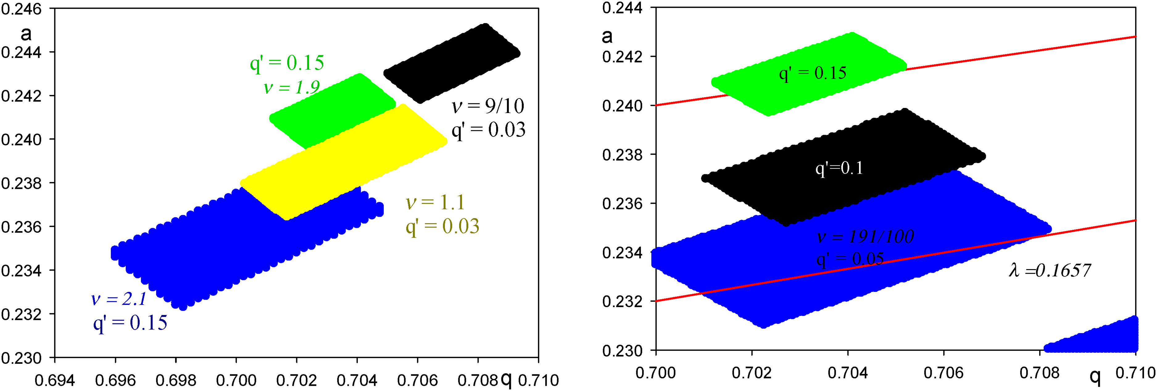
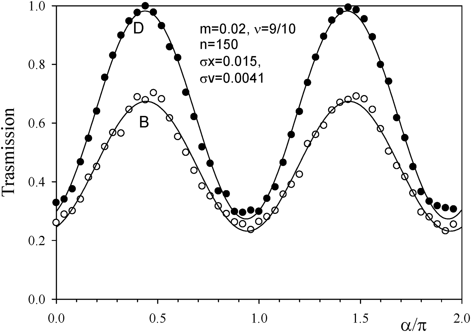
(a) Island A for quadrupoles with ideal quadrupole, and with $A_4=0.15,2,2.6$ , and $4\text{\%}$ added octupole fields, with $a>0$ and $a<0$ ( $q_x=0.02$ , $\nu$  = 9/10). ⁷⁵ (b) Transmission versus resolution for a quadrupole with round rods. Operation in upper islands with shown parameters $\nu$ and $q_{ex}$ . ⁷⁵ Curve 1 is for the normal mode operation.

For comparison, Figure 48(b) shows the dependency of the reserpine ions intensity on the resolution of QMF with round rods for four cases: curve 1 is the operation without excitation, others are operations in islands with parameters $\nu =1/10,q_x=0.07$ (curve 2); $\nu =1/15,q_x=0.03$ (curve 3) and $\nu =\frac{9}{10},q_x=0.04$ (curve 4). The best characteristics have islands with excitation frequencies $\nu =1/15$ and $\nu =9/10$ . For $\nu =9/10$ , the transmittance of the analyzer is approximately constant up to $R_{0.5}\cong 1500$ while in the normal mode, the transmission drops approximately by two orders of magnitude.

In another experimental work, ⁷⁵ low excitation frequencies $\nu =1/10,3/40,1/15,1/20$ , and $1/30$ ( $100$ kHz, $75$ kHz, $66.6$ kHz, $50$ kHz, $33.3$ kHz, respectively) were used. With decreasing excitation frequency ν, the resolving power was $R_{0.5}=1740,1940,1960$ , and $2580$ with values of dimensionless excitation amplitude $q_{ex}=0.011,0.008,0.006,0.003$ . The quadrupole contained a 4% hexapole field component. Note that in the usual mode of operation QMS had low transmission and resolution not suitable for practical applications. The use of quadrupole excitation at low frequencies allows to use quadrupole rod set of low quality and with a low price while providing high-performance characteristics of quadrupole mass spectrometer. ⁵⁶

Here are the results of an experiment in a stability island with a low excitation frequency $\nu =1/30$ . ⁵⁶

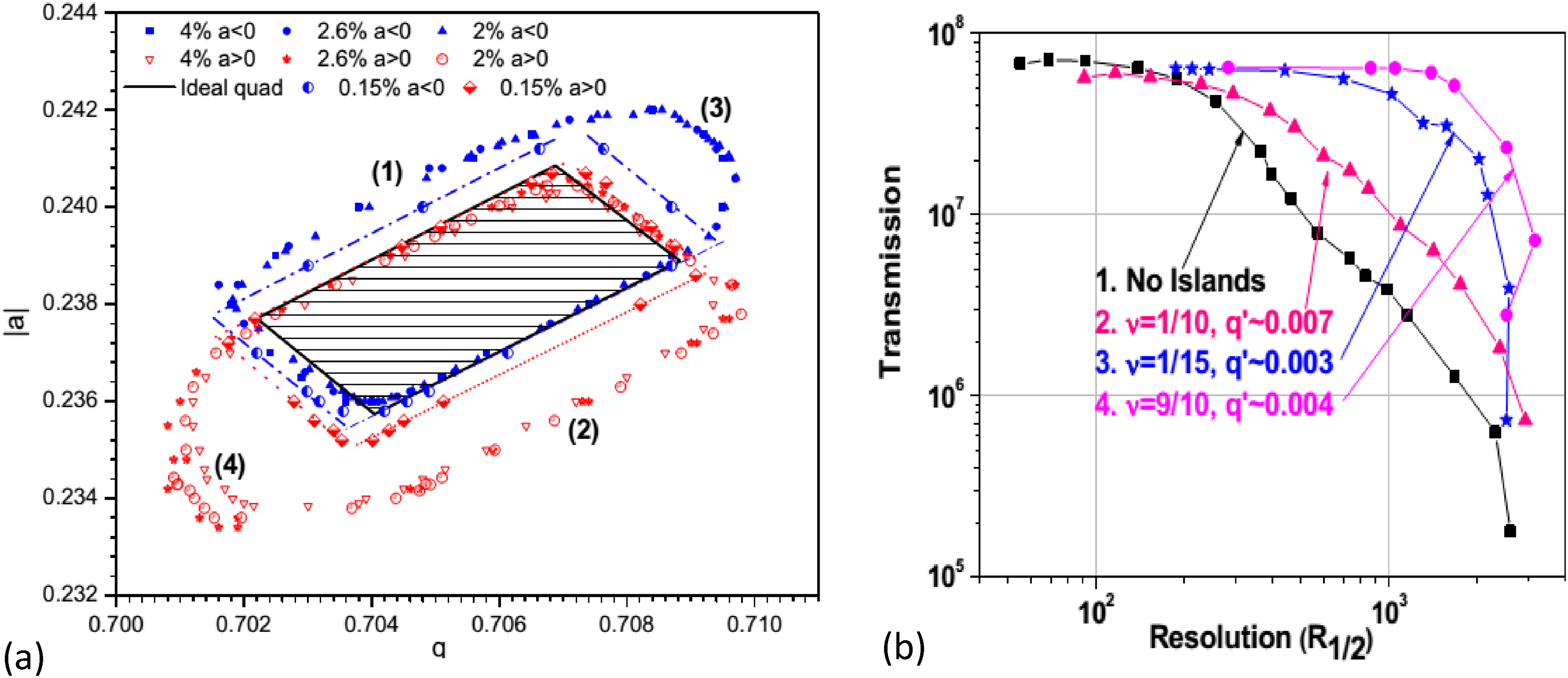
Figure 49 shows the mass spectrum of reserpine during ion separation in the stability island with parameters $\nu =1/30$ and $q_x=0.003$ . The analyzer with round electrodes contained hexapole component $A_3=4\text{\%}$ . The 4A and 4B analyzers had low transmittance, low resolution, and poor peak shape when operated in normal mode (without an island). The use of stability islands dramatically increases resolution and peak shape and, in some cases, transmission.

Figure 49.

Mass spectrum ((a) and (b)) in the stability island excited by an additional quadrupole signal at low frequency $f=33.333$ kHz ( $\nu =1/30$ ) and amplitude $q_x$ = $0.003$ . QMF have had circular electrodes and hexapole field component $A_3=4\text{\%}.$ (c) Conventional mass analysis with the same rod set. ⁵⁶

RF amplitude modulation

For the potential from Eq. 3.14, the ion motion equations in the quadrupole field during modulation of the RF voltage become ⁵⁶

$$\begin{array}{r}{\displaystyle \frac{d^{2}x}{d{t}^2}+[a+2qcos(2(\xi -{\xi }_0))(1+m\cos (2\nu \xi +2\alpha ))]x=0}\end{array}$$

(3.11)

$$\begin{array}{r}{\displaystyle \frac{d^{2}y}{d{t}^2}-[a+2qcos(2(\xi -{\xi }_0))(1+m\cos (2\nu \xi +2\alpha ))]y=0}\end{array}$$

(3.12)

Parameters $a,q,\xi ,\nu ,\alpha$ are defined by formulas (3.1), as in the case of the auxiliary quadrupole potential, m is the modulation index.

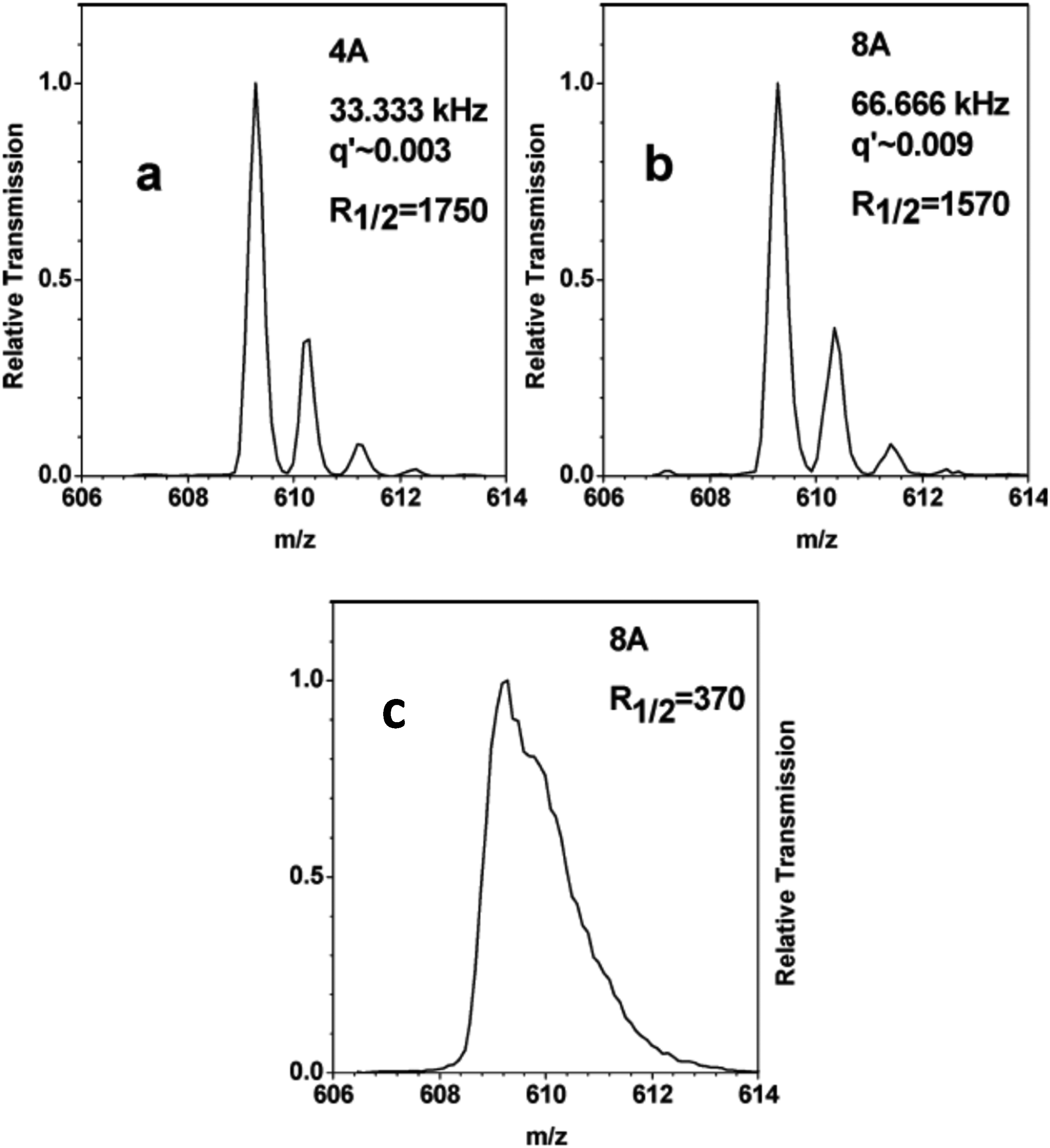
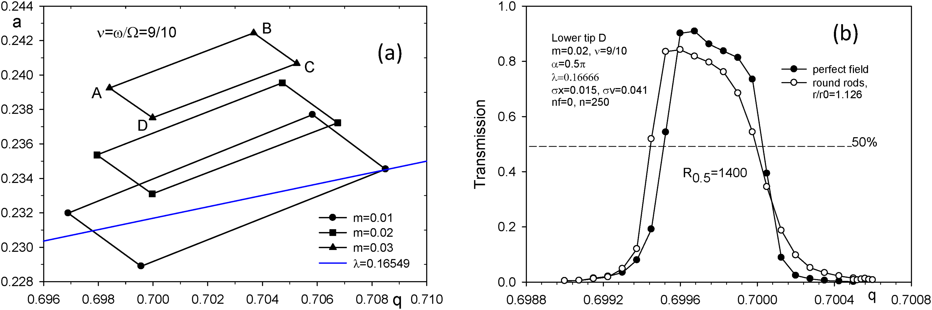
Figure 50(a) shows positions of islands on the $a,q$ plane for values of modulation index $m=0.011,m=0.02$ and $m=0.03$ . Increase of index m leads to area reduction of stability quadrangle and its displacement mainly along the a axis. The operation in the island with variable resolution is possible in two vertices, the lower D and the upper B by changing the slope of the scanning line $a=2\lambda q$ . In the lower tip, the resolution increases when the scanning parameter $\lambda =U/V$ decreases. To work in this island, it is necessary to keep the frequency ν and the modulation index m constant.

Figure 50.

(a) Stability islands created by amplitude modulation at $\nu =9/10$ , at the indicated values of the modulation index m; (b) shape of the mass peak for the ideal field and the field produced by circular rods when operating at the bottom apex D of the stability island with $m=0.02,\nu =9/10$ . Modeling conditions: phase shift $\alpha =\pi /2,$ scanning parameter $\lambda =0.16666$ , standard deviations of initial transverse coordinates ${\sigma }_x=0.015r_0$ and velocities ${\sigma }_v=0.041\pi r_{0}f$ , separation time is $n=250$ RF cycles. ⁷⁶

The shape of the mass peak at the low tip D of the island ( $\nu =9/10,m=0.02$ ) for the rod set with hyperbolic (perfect field) and circular profile ( $r/r_0=1.126$ ) electrodes is shown in Figure 50(b). The input ion beam parameters are described by a Gaussian random distribution with standard deviations ${\sigma }_x=0.015r_0$ and ${\sigma }_v=0.041\pi r_{0}f$ . One can see a weak difference between the mass peaks for the ideal field and the field created by circular rods. This is a strong difference for the normal separation mode in the first stability region. A resolution of $R_{0.5}\cong 1400$ is achieved at transmittance of about 90%. The phase shift $\alpha =\pi /2$ at which the maximum transmittance is achieved is shown here. With amplitude modulation, the phase difference has a strong influence on the transmittance, which is illustrated in Figure 51. The transmittance varies periodically with a phase shift of ( $-\pi ,\pi$ ), since the RF voltage period is also equal to π. The maximum transmittance for vertices D and B is reached at $\alpha =\pi /2$ . The best resolution and transmission is achieved in the lower tip D.

Figure 51.

Transmission dependency on the phase shift α between the RF voltage and the modulating signal at the tips of the island B and D. ⁷⁶

Phase modulation

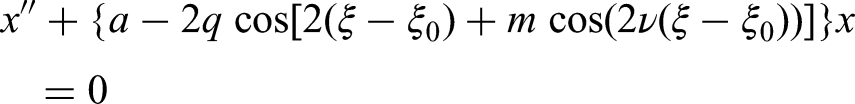
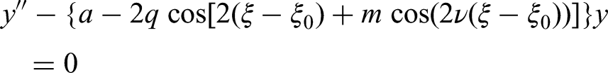
The phase modulation of RF voltage $V\cos \mathrm{\Omega }t$ for the purpose of creating stability islands and modeling their ion-optical properties is considered in reference. ⁷⁷ When the QMF potential (3.17) is applied to the electrodes, the ion motion equations take the form

$$x^{\mathrm{″}}+\{a-2q\cos [2(\xi -{\xi }_0)+m\cos (2\nu (\xi -{\xi }_0))]\}x=0$$

(3.13)

$$y^{\mathrm{″}}-\{a-2q\cos [2(\xi -{\xi }_0)+m\cos (2\nu (\xi -{\xi }_0))]\}y=0$$

(3.14)

As earlier, the following notation is used

$$a={\displaystyle \frac{8eU}{m_i{\mathrm{\Omega }}^2{r}_0^2};q={\displaystyle \frac{4eV}{m_i{\mathrm{\Omega }}^2{r}_0^2};\xi ={\displaystyle \frac{\mathrm{\Omega }t}{2};\nu ={\displaystyle \frac{\omega }{\mathrm{\Omega }}}}}}$$

(3.15)

where ${\xi }_0$ is the initial phase of the RF field, $\nu$ is the relative frequency of the modulation signal, m is a modulation parameter, and $\omega$ is the frequency of the modulation signal.

Stability islands created by quadrupole resonant ion excitation by phase modulation of the RF $AC$ potential $Vcos\mathrm{\Omega }t$ are shown in Figure 52(a). The parameters determining the island positions are the modulating signal frequency $\nu =25/13$ and the phase modulation indices $m=0.170-0.195$ . At such a large value of the modulation index narrow stability bands are formed, which are simultaneously crossed by the scanning line $a=2\lambda q$ with the scanning parameter $\lambda =0.1537$ . It means that by fixing $\lambda$ , the resolution can be increased by increasing the modulation index. This is illustrated in Figure 52(b), which shows mass peaks with a high resolution of $R_{0.1}\cong 6000$ , defined by a 10% peak height but a low transmission of 13–18%.

Figure 52.

(a) The position of X-island in dependence of the modulation parameter m on $a,q$ plane. (b) Calculated mass peaks for $\nu =25/13$ for showing values m, $1000$ trajectories per point. The separation time $n=150$ RF cycles. Standard deviations of velocity ${\sigma }_v=0.0105$ and initial position ${\sigma }_x=0.01$ in relative units, $1000$ trajectories per point. ⁷⁷

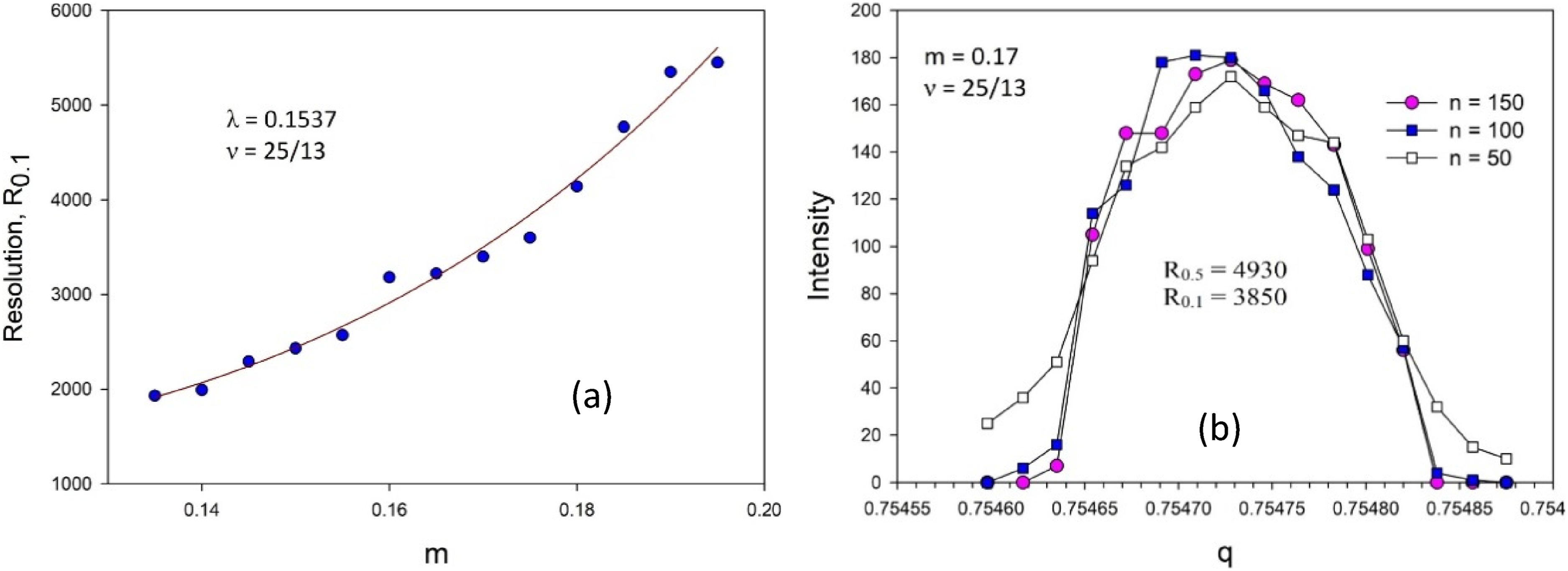
Figure 53(a) illustrates high resolution for the quadrupole, showing the dependence of the resolution $R_{0.1}$ on the phase modulation index m. The effect of the separation time n on the shape of the mass peak is shown in Figure 53(b). It can be seen that an analyzer flight time of only 100 RF cycles is sufficient to achieve a resolution of $R_{0.1}\sim 4000$ .

Figure 53.

(a) Dependence of the resolution $R_{0.1}$ on the modulation index m for an island with $\nu =25/13$ for the constant scanning parameter λ=0.1537. (b) Transmission contours (mass peaks) in the stability island ( $m=0.17$ , $\nu =25/13$ ) for three separation time values $n=50,100,150$ , expressed in number of RF field periods.

The use of RF oscillator phase modulation for ion separation in quadrupole mass spectrometer is limited by the complexity of electronics, when the phase modulation index is $m=0.15$ . For a 1 MHz oscillator with an amplitude $V=3$ kB the modulation frequency would be ∼2 MHz.

Two-frequency quadrupole excitation

M. Sudakov et al.^78,79 suggested to use an auxiliary quadrupole two-frequency excitation to form the upper stability island. Near the working tip of the diagram of the first stability region, the values of the stability parameters ${\beta }_x$ and ${\beta }_y$ can be represented as

$${\beta }_x={\displaystyle \frac{P-1}{P},{\beta }_y={\displaystyle \frac{1}{P},P\sim 10-40}}$$

(3.16)

If the number P is an integer, the oscillations along the x and y coordinates will be periodic with a period $\pi P$ . Denote $\nu =1/P$ . The parametric resonance excitation conditions (3.3) for the x and y directions at $K=1$ are

$${\nu }_{n,x}=|n+1-\nu |,{\nu }_{n,y}=|n+\nu |,n=\pm 0,\pm 1,\dots$$

(3.17)

From here we obtain the combinations of the two resonant frequencies for $n=0$ :

$${\nu }_1={\nu }_{0,x}=1-\nu {\nu }_2={\nu }_{0,y}=\nu$$

(3.18)

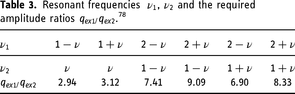
For small values of n, the possible combinations of frequencies ${\nu }_1$ and ${\nu }_2$ are presented in Table 3.

Table 3.

Resonant frequencies ${\nu }_1$ , ${\nu }_2$ and the required amplitude ratios $q_{ex1/}{q}_{ex2}$ . ⁷⁸

${\nu }_1$	$1-\nu$	$1+\nu$	$2-\nu$	$2+\nu$	$2-\nu$	$2+\nu$
${\nu }_2$	$\nu$	$\nu$	$1-\nu$	$1-\nu$	$1+\nu$	$1+\nu$
$q_{ex1/}{q}_{ex2}$	2.94	3.12	7.41	9.09	6.90	8.33

For each combination of frequencies, Table 3 shows the ratio of dimensionless amplitudes $q_{ex1/}{q}_{ex2}$ of the two resonant AC potentials. This result was obtained by direct calculation of stability diagrams for rational frequency values $\nu$ . ⁷⁸ This approach is time-consuming, other ways of calculating the required $q_{ex1/}{q}_{ex2}$ ratios are unknown.

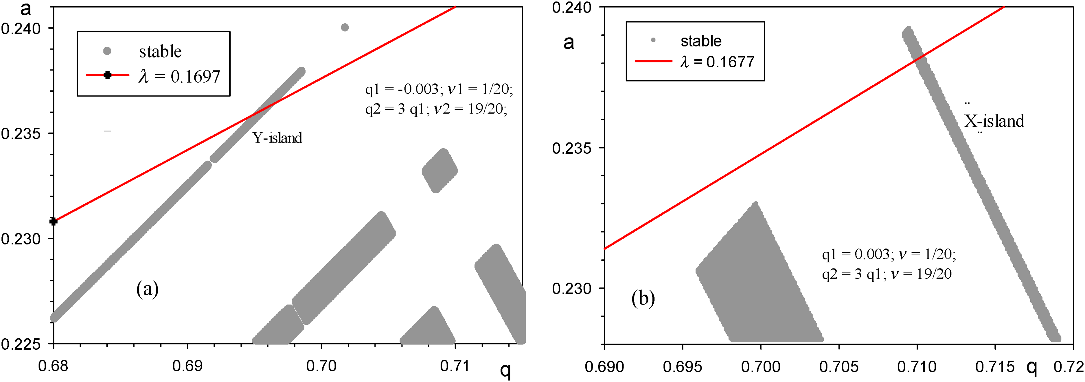
Stability islands formed by two-frequency auxiliary quadrupole AC potentials are shown in Figure 54. Resonant excitation at frequency ${\nu }_1=\nu$ on the Y coordinate and at frequency ${\nu }_2=1-\nu$ on the X coordinate results in narrow bands separated by broad bands of instability. When additional potentials are applied in antiphase $q_1=-q_2$ , there is a narrow band following along the ${\beta }_y$ isoline (Figure 54(a)) and when $q_1=q_2$ , a working X-band following along the ${\beta }_y$ isoline (Figure 54(b)) is created. The advantage of two-frequency excitation over single-frequency one is that X-band is located far from neighboring islands and the scan line $a=2\lambda q$ crosses this band at right angle.

Figure 54.

Stability islands with frequencies ${\nu }_1=1/20,{\nu }_2=19/20$ and excitation amplitudes $q_1=-0.003(a)$ and $q_1=0.003(b),q_2=3q_1$ .

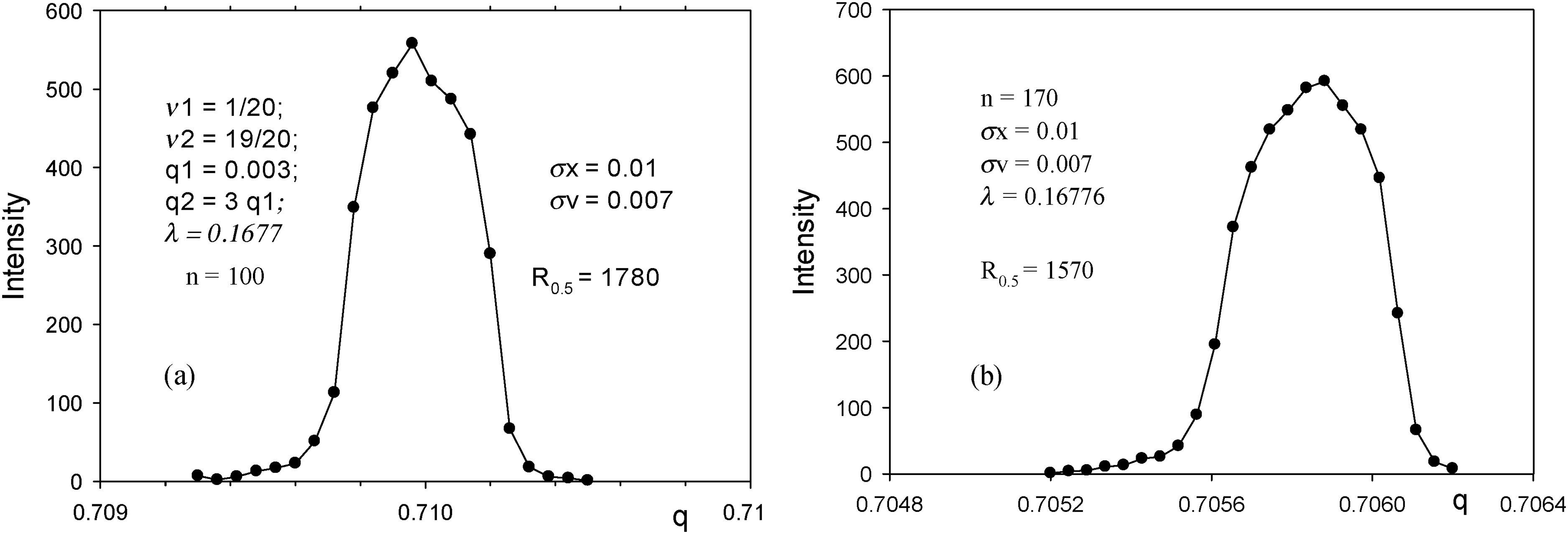
For comparison, Figure 55 shows mass peaks with approximately the same intensities. The transmission in both cases is approximately 60%. The resolution is slightly higher for the X island (Figure 54(b)). The most important difference for Figure 55 for (a) and (b) is that the required separation time is $n=100$ and $n=170$ . Assuming that the resolution $R\sim n^2$ ³⁶ the gain in electrode length for the new mode of operation is ${\left(\frac{170}{100}\right)}^2\cong 2.9$ times. This means that it is possible to reduce the electrode length, for example, from $200$ mm to $80$ mm to achieve the same performance as in the normal QMF operating mode.

Figure 55.

Calculated mass peaks at the same initial conditions ${\sigma }_x=0.01r_0,{\sigma }_v=0.007\pi r_0$ . (a) X-island mode operation, (b) standard mode operation.

Conclusions

Modeling linear ion traps. The excitation contour is a convenient method to describe the phenomenon of dipole resonance excitation of ion oscillations. The formula for the resolving power does not take into account such factors as quadrupole acceptance, spatial charge, and pressure. Nevertheless, it does take into account the main factors of the resonance process, the contour broadening over a finite excitation time of the ion ensemble and the dispersion between the ion mass and the excitation frequency. There is an excellent agreement between the simulation and formula for resolving power. In the case of DE, excitation time n and amplitude $q_{ex}$ are strongly coupled as $q_{ex}\sim 1/n$ . Achieving high resolution ( $R_{0.5}=30,000$ ) with a buffer gas requires maintaining high stability of the $q_{ex}$ amplitude and pressure. The main drive rectangular wave voltage with sinusoidal wave dipole signal provides approximately the same resolution at the specified pulse waveform.

The optimal values of $r/r_0$ for the QMF with circular electrodes are $\cong 1.10-1.130$ and for the LIT $r/r_0\cong 1.15-1.17$ . Quadrupole excitation has a lower resolving power because the quadrupole force acting on the ion is proportional to the ion shift, while the force from the DE is independent of coordinate. However, the presence of the octupole field component with $A_4\cong 4\text{\%}$ increases the mass selectivity of quadrupole excitation. Two-frequency excitation simulations reveal the nature of the reduced spatial charge effect, namely, that there are two competing resonance processes in nonlinear quadrupole fields. The application of the second stability region for mass-selective resonant ion ejection from a linear ion trap is problematic. Strong localization and cooling of the ion cloud in the near-axis region is necessary before ions are ejected from the trap. Small radial dimensions of the cloud with high ion concentration before the ejection of ions from the trap leads to a spatial charge effect. The efficiency of ion trapping in a linear trap depends on the phase volume characterized by the acceptance of the linear quadrupole. The trap acceptance is largely controlled by the fringing fields. Therefore, ion focusing is necessary when injecting the ion beam into the linear trap by the above methods. The influence of the fringing fields on the process of resonant excitation of ion oscillations requires additional studies.

Quadrupole mass filter with dipole excitation. The excitation contour is a convenient method to describe the phenomenon of dipole and quadrupole resonance excitation of ion oscillations. The formula for the resolving power does not take into account such factors as quadrupole acceptance, spatial charge, and pressure. Nevertheless, it does take into account the main factors of the resonance process, the contour broadening over a finite excitation time of the ion ensemble and the dispersion between the ion mass and the excitation frequency. There is an excellent agreement between the simulation and formula for resolving power. In the case of DE, excitation time n and amplitude $q_{ex}$ are strongly coupled as $q_{ex}\sim 1/n$ . Achieving high resolution ( $R_{0.5}=30,000$ ) with a buffer gas requires maintaining high stability of the $q_{ex}$ amplitude and pressure. The main drive rectangular wave voltage with sinusoidal wave dipole signal provides approximately the same resolution at the specified pulse waveform.

The optimal values of $r/r_0$ for the QMF with circular electrodes are $\cong 1.10-1.130$ and for the LIT $r/r_0\cong 1.15-1.17$ . Quadrupole excitation has a lower resolving power because the quadrupole force acting on the ion is proportional to the ion shift, while the force from the DE is independent of coordinate. However, the presence of the octupole field component with $A_4\cong 4\text{\%}$ increases the mass selectivity of quadrupole excitation. Two-frequency excitation simulations reveal the nature of the reduced spatial charge effect, namely, that there are two competing resonance processes in nonlinear quadrupole fields.

The application of the second stability region for mass-selective resonant ion ejection from a linear ion trap is problematic due to LIT acceptance. Strong localization and cooling of the ion cloud in the near-axis region is necessary before ions are ejected from the trap.

Quadrupole mass filter with quadrupole excitation. Quadrupole parametric resonant excitation allows improvement QMF characteristics. This requires a significant complication of the RF oscillator electronics.

The presence of stability islands under quadrupole excitation has been proved experimentally and perfectly agrees with theoretical study of the Hill equation. Methods of quadrupole excitation by auxiliary RF voltage, amplitude, phase, and frequency modulation of sinusoidal and rectangular waveform-driven voltage are described. An approach for mapping of stability islands based on the numerical solution of the Hill equation of ion motion in the presence of quadrupole excitation works effectively for all excitation methods. The resonant frequencies of quadrupole excitation are determined based on the classical parametric resonance condition.

It is shown experimentally that in the presence of a 2% octupole field component, the best results are obtained at excitation frequencies $\nu =1/15$ and $\nu =9/10$ . An analyzer with circular electrodes with hexapole spatial harmonic field (4%) in the normal mode provides a resolution of $R_{0.5}=80$ , while with quadrupole excitation at frequency $\nu =1/30$ a resolution of $R_{0.5}=2950$ is achieved. This means that it is possible to use rod set constructed with lower mechanical tolerances. Dual-frequency quadrupole excitation is technically the most complicated operation mode and reveals excellent mass separation properties: resolution is about 1700 and transmission 50% in case of absent fringing fields. Trajectories numerical simulation with quadrupole excitation show that rod length may be reduced in 2–3 times in compare with normal mode operation for the same resolution.

Phase and amplitude modulation of the quadrupole voltage has not been experimentally studied due to the complexity of the electronics. Modeling quadrupole excitation by means of phase modulation showed that the peak shape is relatively weakly affected by the instability of supply voltages at high resolution $R_{0.1}\sim 4000$ .

In the case of amplitude modulation, the most effective QMF operation is in the lower tip of the stability island, with the transmittance periodically changing with the phase of the modulating signal. The problem of fringing input fields remains as in the case of the conventional QMF operation.