
Abstract
One promising approach to reduce carbon foot print of internal combustion engines (ICEs) is using alternative fuels like hydrogen, particularly by converting medium and heavy-duty diesel engines to dual-fuel hydrogen-diesel engines. To minimize elevated NOx emissions from hydrogen-fueled engine, fast and accurate emission models are essential for engine model-based control and for engine calibration and optimization using hardware-in-the-loop (HIL) setups. In this study, a fast-response NOx emissions sensor is used to measure the transient NOx emissions from a dual-fuel hydrogen-diesel engine. Subsequently, steady-state models (SSMs), quasi steady-state models (QSSMs), and transient sequential models (TSMs) in the form of black-box (BB) and gray-box (GB) models are developed for transient NOx emissions prediction. GB models utilize both information from a one dimensional (1D) physical engine model and experimental data for training, while BB models only use experimental data. SSMs are optimized artificial neural networks (ANNs) trained using steady-state data, QSSMs are optimized ANNs trained using transient data, and TSMs are time-series networks trained using transient data. Long short-term memory (LSTM) and gated recurrent unit (GRU) networks are used as the time-series deep learning networks. The results showed that the 1D physical model has the poorest performance with successive model performance improvement from SSM to QSSM and from QSSM to TSM. The developed BB TSM model in this study can predict transient NOx emissions with an R2 value greater than 0.96 at 89,000 predictions per second which makes this model suitable for real-time engine model-based control where computational efficiency is crucial. The developed GB TSM model can predict transient NOx emissions with an R2 value greater than 0.97 but it is computationally more expensive. The extra accuracy of the GB TSM models makes them the best choice for HIL setups where more computational power is available, and accuracy is more crucial.
Keywords
Introduction
According to national inventory of Canada, carbon dioxide
Hydrogen is considered a promising alternative fuel source due to its unique properties. It is a clean energy source as it results in zero carbon engine-out emissions and can be produced using renewable energies. 3 Additionally, its low ignition energy means that it can ignite quickly and burn cleanly, while its rapid flame propagation ensures efficient combustion. 3 Compression ignition engines, also known as diesel engines, have limitations when it comes to running solely on hydrogen fuel. The compression temperature in these engines is usually not high enough to initiate combustion of hydrogen.3,5 As a result, diesel engines are unable to directly use hydrogen as the sole fuel source. 5 However, these engines can be converted with minimum changes to the engine to dual-fuel hydrogen-diesel where the diesel fuel ignites the premixed mixture of hydrogen-air.5–7
Adding hydrogen to CI engines increases the combustion temperature, resulting in the production of higher levels of nitrogen oxides
This study aims to address the following research gaps based on the current literature in
The current literature is abundant in transient emission studies for traditional SI and CI internal combustion engines (ICEs) fueled by fossil fuels. However, there is a significant lack of research on transient emission modeling for engines utilizing alternative fuels. This gap in the literature is particularly important for engines fueled by hydrogen, as the addition of hydrogen is known to increase combustion temperatures and
Data-driven modeling of transient emissions can be accomplished through the use of three main methodologies: SSM, QSSM, and TSM. While some studies have compared the performance of two of these methods, there is a lack of research that has investigated and compared the performance of all three models for the same engine and the same dataset. This study compares the performance of SSM, QSSM, and TSM methodologies on both steady-state and transient
The use of gray-box (GB) emission modeling has been demonstrated to enhance steady-state emission modeling11–15; however, the application of GB modeling for transient emission modeling remains unexplored in the literature. This study investigates the use of GB modeling technique in the form of SSM, QSSM, TSM, for modeling transient
In the context of engine model-based control, having a computationally efficient accurate emission model is crucial. To address this need, this study investigates a range of different architectures and algorithms for time-series TSM modeling and compares their performance in terms of both accuracy and computational cost. By doing so, this study provides valuable guidance on how to choose the most appropriate TSM model-based on the desired trade-off between accuracy and computational cost, taking into consideration the available computational resources. The results of this study can help researchers and practitioners make informed decisions about which TSM model is best suited for their particular application, ensuring that the model is both accurate and computationally efficient.
The paper is organized into sections, beginning with a presentation of background studies on
Background NOx emissions modeling studies
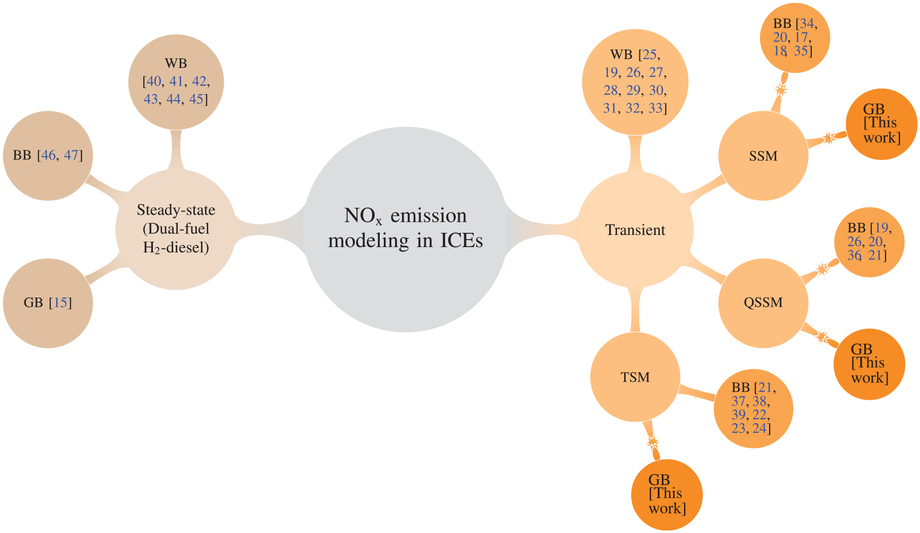
Emissions are often modeled through three main methodologies: physical models or white-box (WB), black-box (BB) models, and GB models. Model-based control requires models to be fast enough for real-time emission prediction. This consideration makes complex and accurate physical models not applicable, and only low dimensional and empirical physical models can be used in this application. 16 BB models are machine learning (ML) algorithms that are trained using experimental data. Simulation data can also be used for BB modeling, but it will lower the accuracy of the model depending on the accuracy of the simulation data. One advantage of BB models is that they are significantly faster compared to physical models. Finally, GB models are a combination of the WB and BB modeling, where a combination of data from a physical model and experimental data is used for training an ML method. GB models can be as fast as low dimensional physical models and more accurate than BB models because they use extra information provided by the physical model.11–14
ML algorithms can be utilized for transient emission modeling through GB and BB models in three distinct ways, depending on the algorithm type and the source of the training data. The most straightforward approach in transient emission modeling is to utilize steady-state emission models (SSM). These models consist of a classical ML algorithm that has been trained using steady-state emission data, and are now applied for the prediction of transient emissions. Due to the lack of transient emission data in the training process, these models have limited capacity to accurately predict the emissions. GB version of these models can perform better to a certain extent depending on the accuracy of the physical model. This is because the physical model can provide additional information and incorporate certain elements of the transient nature of transient emissions into the ML method. In Norouzi et al.
17
and Aliramezani et al.
18
support vector machine (SVM) algorithm was trained using steady-state data for predicting
The second approach for utilizing ML in transient emission modeling involves training classical ML algorithms with transient emission data. In this methodology, the emission value at each time step is treated as an individual steady-state case during the training process. These models are referred to as quasi steady-state models (QSSMs) and have the advantage of using the same type of data for both training and testing. However, the disadvantage of these models is that they cannot account for the sequential nature of transient emissions. This means for predicting each case algorithm only relies on the current state and not the previous states, which does not reflect the reality of transient emissions. Similar to SSMs, the performance of QSSMs can be improved through the implementation of a GB version, as the physical model can provide additional information and capture some aspects of the transient behavior. In Jeyamoorthy et al.,
19
QSSM models for
The third strategy for modeling transient emissions using ML methods involves the use of transient sequential models (TSMs). In this approach, a deep learning (DL) recurrent neural network (RNN) is trained using transient emission data. RNNs have the capability to capture the sequential nature of transient emissions, meaning that the emission value at each time step depends on both the inputs at the current time step and the previous time steps. Two of the most widely used types of RNNs are long short-term memory (LSTM) and gated recurrent unit (GRU). These models can effectively handle the time-series nature of the data and can provide improved predictions of transient emissions compared to traditional models.
8
In Moradi et al.,
21
both QSSM and TSM are developed for predicting transient
Prior
Methodology
This section explains the experimental setup, physical model that is used for GB modeling, and also ML, DL, and FS algorithms that are used in this study.
Experimental setup
The dual-fuel hydrogen-diesel engine used in this study is a medium-duty CI diesel engine13,14 that has been modified through the addition of a hydrogen injector in the intake manifold.
15
To accurately measure the emissions from the dual-fuel operation, sensors have been installed on the separate exhaust of the dual-fuel cylinder, while the other cylinders continue to operate on diesel fuel only. The injection timing of the hydrogen is precisely coordinated with the valve timing of the target cylinder to ensure all of the injected hydrogen goes to the target cylinder.
13
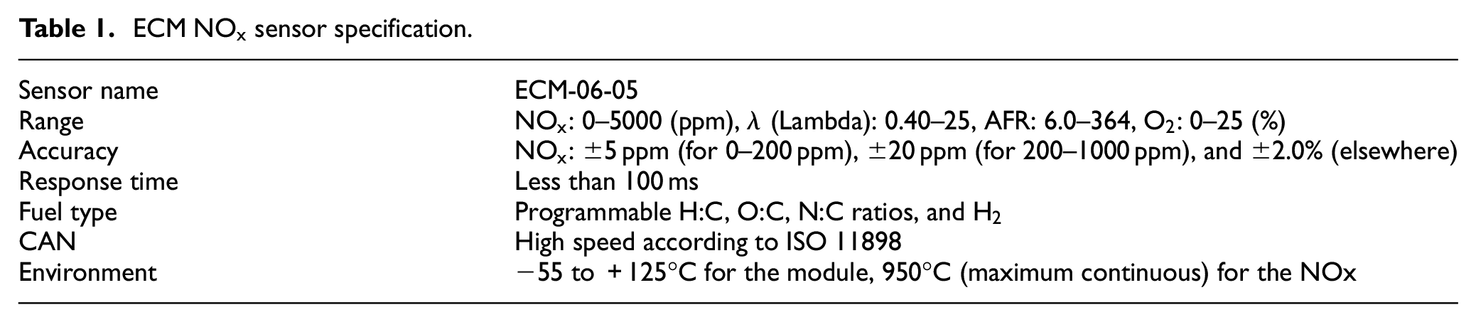
The experimental setup for the engine, including the NOx emissions measurement sensor are shown in Figure 2. The properties and specifications of the NOx sensor used for measuring transient NOx emissions are provided in Table 1 with more details on the sensor available.48–51 The engine experimental setup was utilized to measure NOx emissions over 82,300 engine cycles at a constant engine speed of 1500 rpm and without exhaust gas re-circulation (EGR). This dataset includes duration of over 6500 s. Implementing EGR and other after-treatment systems can reduce output
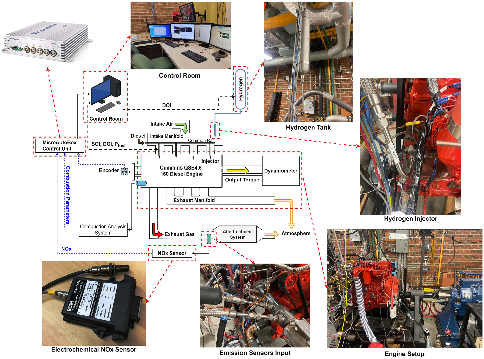
ECM
To control combustion, this diesel engine employs two diesel injection pulses - a short pilot injection and a longer main diesel injection. Figure 3 shows the injection setting in this study. The control injection parameters in the experimental tests are: (i) the crank angle at the start of injection for pulse 1
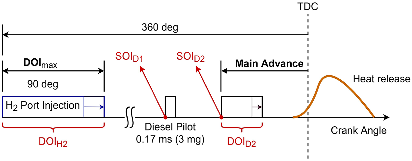
Hydrogen and diesel injection setting in this study. Injection control parameters are shown in red.
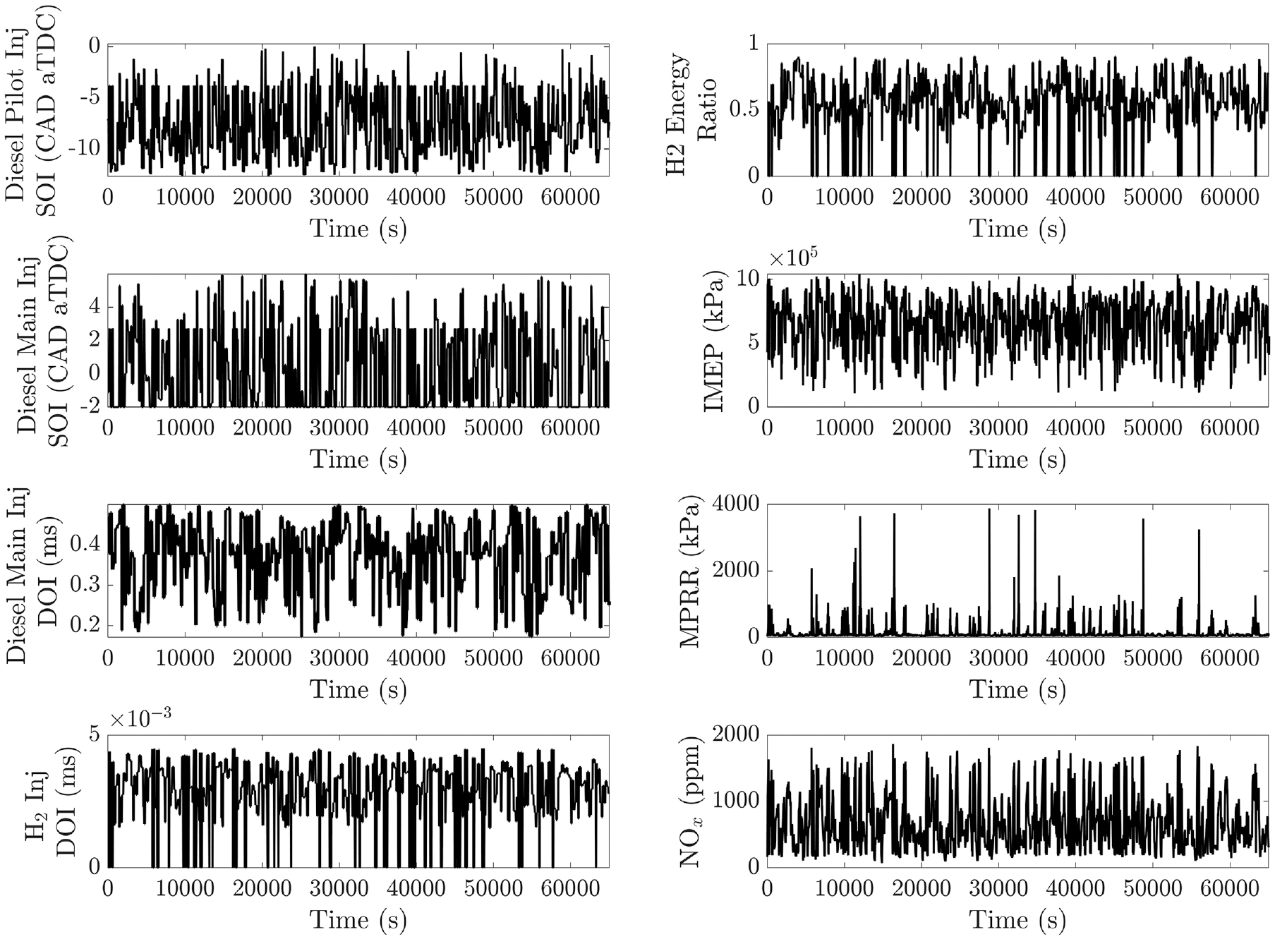
Dual-fuel compression ignition hydrogen-diesel engine experimental data over 82,300 engine cycles at constant engine speed of 1500 rpm and without EGR. MPRR stands for maximum pressure raise rate.
Physical model
The physical model or WB model for the dual-fuel hydrogen-diesel was created using the dual-fuel combustion model in the GT-Power software. This model is a combination of direct-injection diesel multi-pulse and SI combustion model that is designed for dual-fuel SI-CI combustion. The cylinder contents in the model are divided into three thermodynamic zones with distinct compositions and temperatures. These include an unburned zone, a spray zone with injected fuel and entrained gas, and a spray burned zone with combustion products. The combustion rate is predicted based on the amount of unburned mixture behind the flame front, which is influenced by the sum of the turbulent flame speed (TFS) and the flame area. ML laminar flame speed (LFS) models 52 are used for LFS calculation which is then used to calculate TFS.
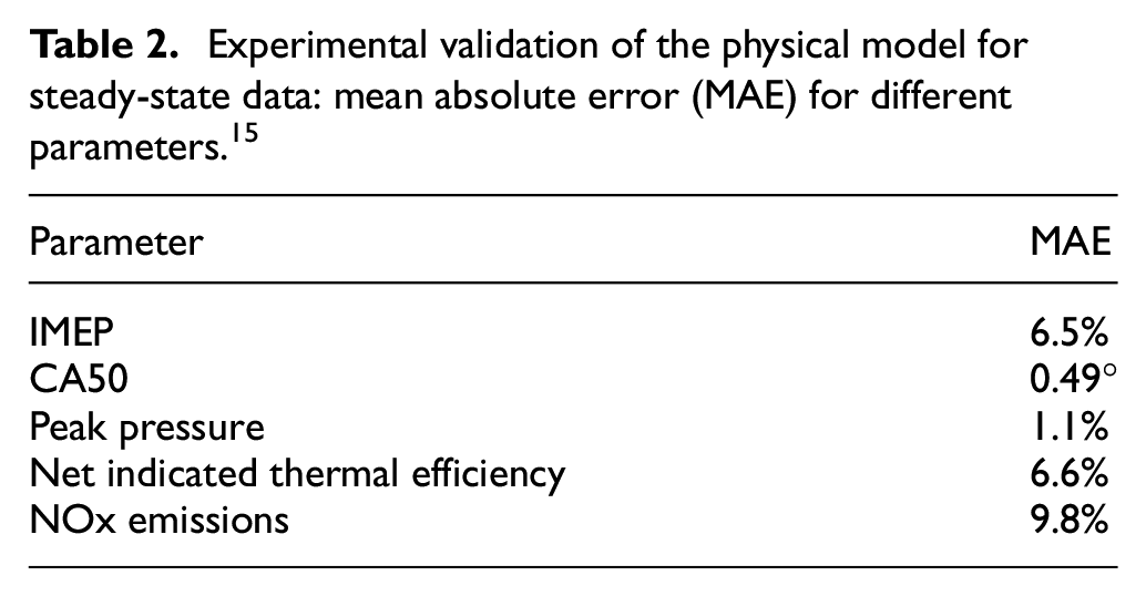
The dual-fuel combustion model in the GT-Power software has 7 calibration parameters, which are carefully adjusted to optimize the model’s accuracy and predict the combustion rate of the dual-fuel engine with a pilot injection. The first three parameters are related to the simulation of SI combustion, including the turbulent flame speed multiplier, the Taylor length scale multiplier, and the flame kernel growth multiplier. These parameters affect the turbulent flame speed and, in turn, the burn rate and in-cylinder pressure. The remaining four parameters are related to the ignition process of the dual-fuel combustion and include the entrainment rate multiplier, the ignition delay multiplier, the premixed combustion rate multiplier, and the diffusion combustion rate multiplier. A genetic algorithm was utilized for optimal tuning of the calibration parameters based on the experimental in-cylinder pressure traces for the 79 steady-state measurements. 15 Table 2 presents the validation of the physical model using experimental steady-state data for various parameters. Figure 5 illustrates a comparison between the experimental and physical model in-cylinder pressure trace for three steady-state cases. Further details about the physical model validation can be found in the previous study. 15
Experimental validation of the physical model for steady-state data: mean absolute error (MAE) for different parameters. 15
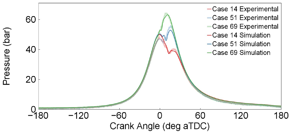
Experimental validation of the physical model in predicting in-cylinder pressure traces for three steady-state cases. 15
In this study, the physical model is used for GB modeling. To do this, the physical model produces physical outputs for each engine case. The physical outputs are then selected through a combination of expert knowledge and FS algorithms. The selected outputs form the training data for the ML algorithm, resulting in a gray-box (GB) model that is trained using a wider range of input parameters compared to black-box (BB) models. BB models are only trained using four main inputs (
In contrast, GB models in this study are built using a robust physical model and trained with a broader range of physically calculated input features. This allows GB models to perform better on data outside the training range, as they incorporate physical understanding in output prediction rather than relying solely on extrapolation like BB models. This is one of the main advantages of GB models over BB models.
Machine learning and deep learning methods
ML models are now employed for predicting NOx emissions through three methodologies: SSM, QSSM, and TSM. A fully connected ANN was selected as the classical ML approach for SSM and QSSM, as it has been proven in previous studies13,15 that optimized ANNs can outperform other classical ML algorithms such as SVM, RF, GPR, and Ensemble of Regression Trees. The hyperparameters of the ANN model, including the number of hidden layers, the number of hidden neurons per layer, and the regularization parameter
The SSM models were trained and validated using 79 steady-state cases of dual-fuel hydrogen-diesel engine at constant speed of 1500 rpm. For the QSSMs, over 82,300 transient cycles (Figure 4) were used, with 70% of the data designated for training, 15% for validation, and 15% for testing. The QSSMs were trained using the training data and the best models were selected based on their performance on the validation set. Finally, the models were tested using the test data which was not used for training or validation.
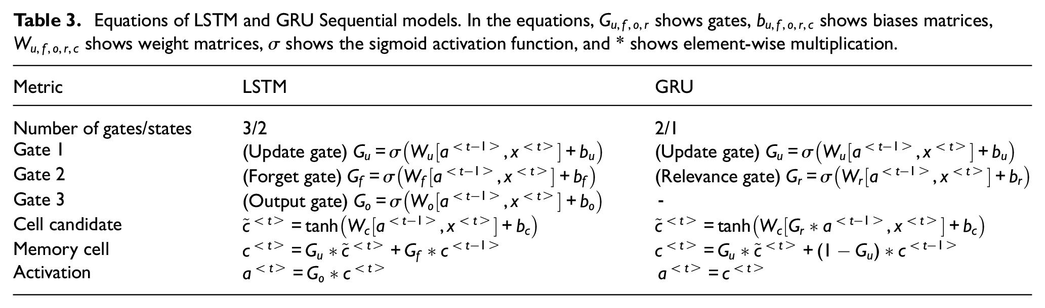
TSM models use time series sequential ML algorithms, such as LSTM and GRU networks, which are RNN algorithms that use gates to overcome the vanishing gradient problem. A GRU network
53
has two gates, a relevance gate, and an update gate, along with one memory cell
Equations of LSTM and GRU Sequential models. In the equations,
LSTM and GRU networks are employed to construct TSM models for BB and GB NOx emissions. Figure 6 shows the schematic of the BB LSTM and GB GRU TSMs. Similar architectures are also used for the GB LSTM and BB GRU TSMs. As it is seen in Figure 6, the engine simulation model (ESM) acts as an extra layer in the network for the GB models. The TSM network architecture comprises three fully connected layers at the beginning, followed by a time series layer (either LSTM or GRU), a drop-off layer, and an output layer at the end. The drop-off layer randomly deactivates half of the network during each training iteration, thereby reducing overfitting and training computational expenses. This architecture was determined through trial and error and trade-off between complexity and minimizing error. To train these models, MATLAB Deep Learning Toolbox© with the Adam algorithm with mini batch size of 1024 has been used. The training, validation, and test data were similar to those used in QSSMs, and the training process continued until the validation loss consistently started to increase. At that point, the training was halted and the model with the lowest validation loss was chosen
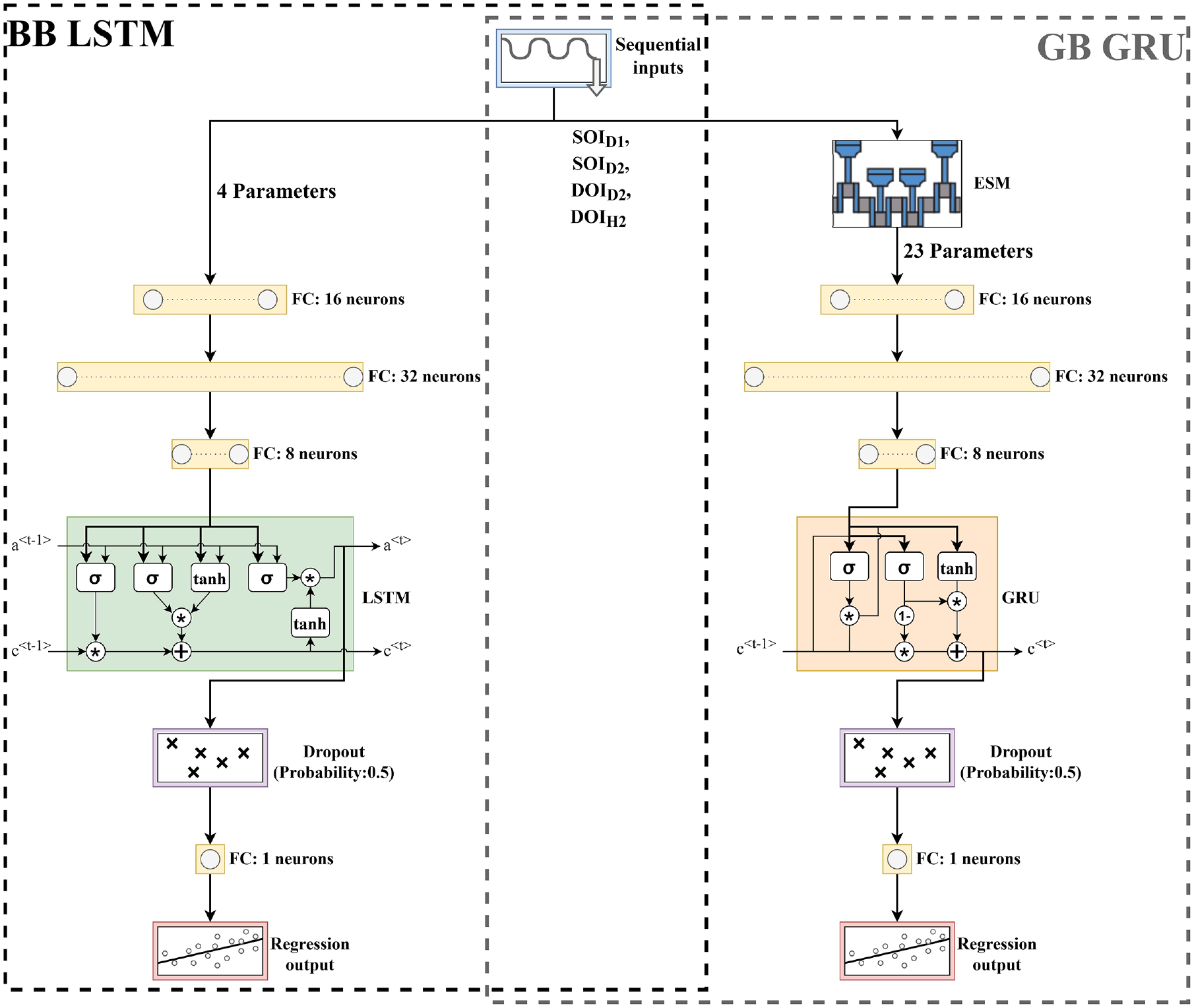
Transient sequential models architecture. Left: BB LSTM model, right: GB GRU model. ESM stands for engine simulation model,
Feature selection
The choice of input feature set is a crucial factor in the performance of the emission modeling GB algorithm. 13 Previous research13,15 has highlighted that relying solely on expert physical knowledge may not be sufficient for selecting the most important physical features for emission modeling. Incorporating ML algorithms for FS in conjunction with expert knowledge has been shown to improve the performance of the GB model. To this end, four FS algorithms (F-test, minimum redundancy maximum relevance (MRMR), RReliefF, and least absolute shrinkage and selection operator (LASSO)) were employed, and their effect on the GB model’s performance was evaluated in comparison to the BB model. Here, each of the FS algorithms that are used in this study are briefly described.
F-test algorithm 55 evaluates the significance of each predictor, which involves comparing the means of response values across different predictor variable values. The p-values derived from these F-test statistics can then be used to rank the features, with higher scores corresponding to lower p-values. Essentially, an F-test examines whether the response values for different predictor variable values are drawn from populations with the same mean or not, and the resulting scores reflect the negative logarithm of the p-values.
The MRMR algorithm
56
aims to identify the most effective set of features that can accurately represent the response variable, while ensuring that the features are both mutually and maximally dissimilar. To achieve this, the algorithm works toward minimizing the redundancy of the selected feature set, while simultaneously maximizing its relevance to the response variable. This is done by quantifying both the redundancy and relevance of the features using mutual information measures, which consider the pairwise mutual information of features as well as the mutual information of a feature with the response variable. The MRMR algorithm
56
is specifically designed for regression problems, and its objective is to identify an optimal feature set S that maximizes the relevance
RReliefF
57
is a weight-based algorithm that determines the importance of predictors when the response variable y is a multi-class categorical variable. The algorithm aims to penalize the predictors that generate different values for observations belonging to the same class while rewarding those that generate different values for observations belonging to different classes. Initially, RReliefF sets all the weights for predictors, denoted as
LASSO13,14 is a type of regression analysis that combines variable selection and regularization to improve the model’s predictive accuracy. Specifically, the LASSO regression incorporates a penalty term, represented by the variable λ, in the cost function to penalize the
Results and discussion
In this study, the input feature set for all BB models was comprised of four features:
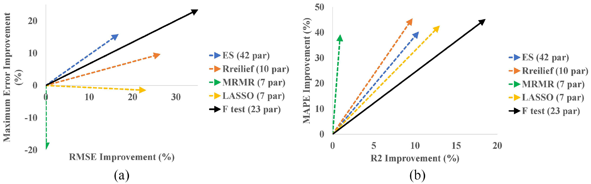
Comparison of black-box quasi steady-state model with gray-box quasi steady-state model with feature selection using different algorithms: (a) maximum error and RMSE improvement compared to black-box model and (b) MAPE and
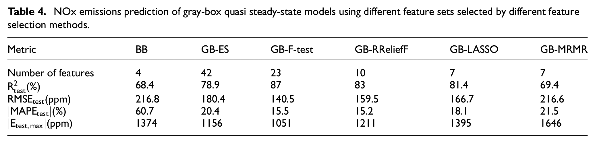
The expert selection (ES) of features, which involves using all features selected based on physical knowledge alone, resulted in a weaker performance compared to most other FS algorithms that combined expert knowledge with ML algorithms. The F-test algorithm outperformed the other FS algorithms, with the highest improvement of RMSE, maximum error, and
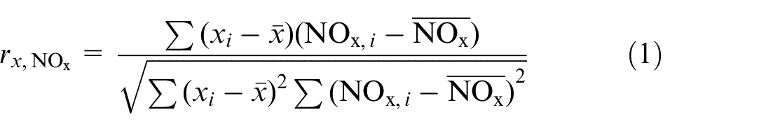
Here,
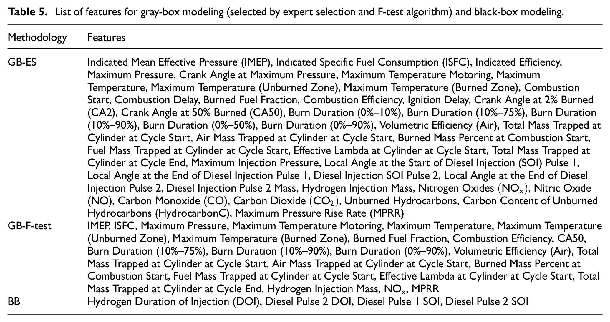
List of features for gray-box modeling (selected by expert selection and F-test algorithm) and black-box modeling.
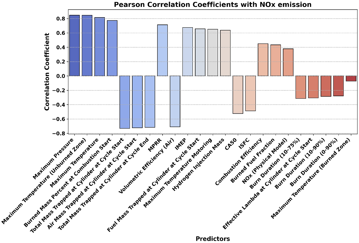
Pearson correlation coefficients of predictors from GB-F-test feature-set with the output (
The F-test algorithm selected almost all of the features chosen by other FS algorithms, and the 23 features it identified were used for QSSMs and TSMs. For SSM, a similar approach was followed, and seven features were selected using the F-test algorithm, as the training dataset for SSM comprised steady-state data.
The number of hidden units in the time series layer is a critical factor that significantly affects the ability of TSMs to capture the sequential nature of the transient emission data. However, a very high number of hidden units can lead to a more complex model that is unsuitable for engine model-based control and might also result in overfitting. To determine the optimal number of hidden units in the time series layer, the BB LSTM architecture (shown in Figure 6) with different numbers of hidden units within the LSTM layer were developed. The training and validation transient NOx emissions dataset were used for this purpose.
As shown in Table 6, increasing the number of hidden units results in a higher number of trainable parameters in the model, which can increase training and prediction time. An increase in the number of hidden units initially leads to a significant improvement in model performance. However, this trend eventually slows down, and after a certain point, increasing the number of hidden units has little to no effect on model performance and may even degrade it.
Effect of hidden unit number on LSTM model performance in NOx emissions prediction. Modeling was carried out using IntelR XeonR CPU E3-1245 V2 @ 3.40 GHz processor and 32 GB RAM.
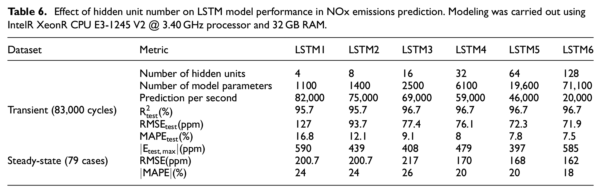
The analysis shows that increasing the number of hidden units up to 16 (as shown in Figure 9) improves model accuracy without significantly affecting computational speed. Increasing the number of hidden units from 16 to 64 slightly improves model accuracy but makes the model slower. Increasing the number of hidden units post 64 only results in a slower model without a corresponding increase in accuracy. Considering the trade-off between accuracy and computation cost, a range of 16–64 hidden units appears to be the optimal choice.
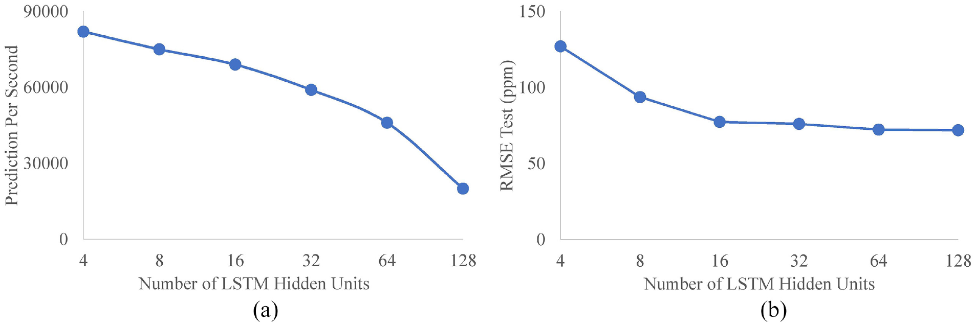
Effect of hidden unit number on the LSTM model’s (a) prediction rate (per second) and (b) RMSE for the test dataset (ppm). The modeling was performed using an Intel® Xeon® CPU E3-1245 V2 @ 3.40 GHz and 32 GB RAM.
Based on this analysis, if accuracy is the most critical factor in the accuracy-computational cost trade-off, the recommended choice would be the LSTM network with 64 hidden units. To investigate the performance of other popular time series network (GRU) and the effects of GB modeling on time series networks, GB LSTM model, BB GRU model and GB GRU model (shown in Figure 6) were modeled with 64 hidden units within the time series layer. Table 7 compares the performance of these four models in terms of model complexity, computational cost, and accuracy.
Comparison of time series networks’ performance for transient and steady-state NOx emission modeling. Modeling was carried out using IntelR XeonR CPU E3-1245 V2 @ 3.40 GHz processor and 32 GB RAM.
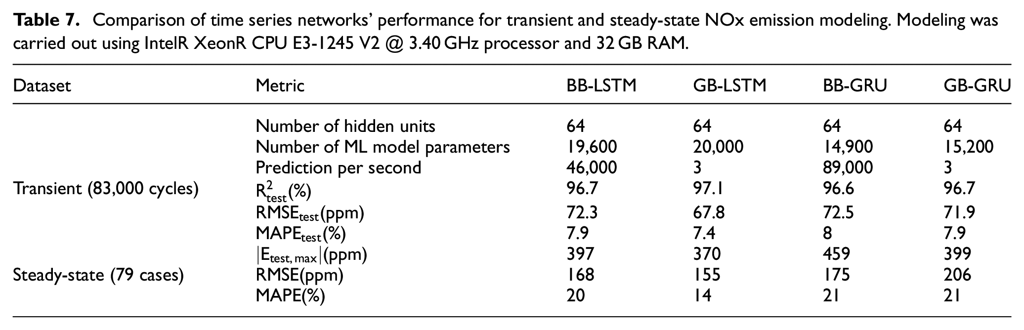
The GRU model has fewer trainable parameters for the same number of units than the LSTM model because it is a simpler version of the LSTM network. This makes the GRU model faster than the LSTM model. However, GB models are much slower in prediction than BB models because the physical model inside the GB models needs to simulate each case and feed the network with its output, making the model considerably slower.
In terms of accuracy, GB LSTM and GB GRU are more accurate than the corresponding BB models. This demonstrates that GB modeling can improve TSMs. However, compared to QSSMs, the difference in accuracy between GB and BB models for time series networks is much smaller. This is because time series networks are DL algorithms that effectively capture the sequential nature of the transient emission, leaving little room for improvement by using additional information provided by physical models in the form of GB models.
The GB LSTM model has the best steady-state and transient performance among the four models. It has the highest
In summary, selecting the appropriate TSM depends on the specific application’s requirements. Here for NOx emissions modeling, the GB LSTM model that can predict transient NOx emissions with
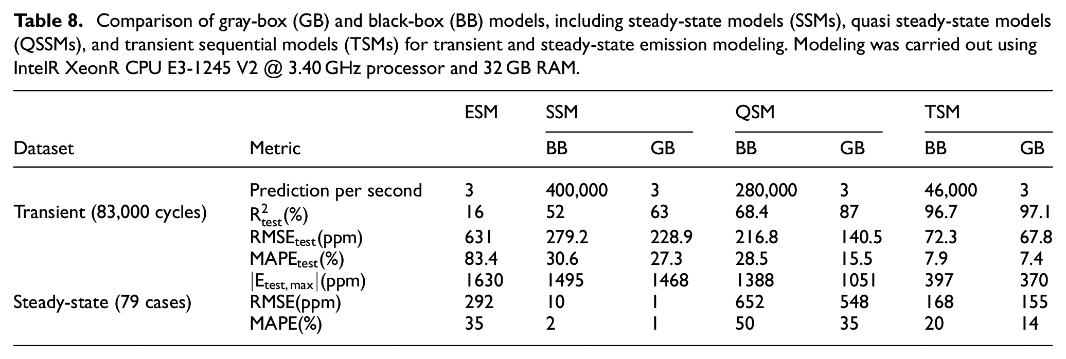
To assess the effectiveness of various modeling methodologies for NOx emissions, Table 8 presents a comparison of ESM, SSMs, OSSMs, and TSMs in terms of their computational cost and performance on both steady-state and transient data. Additionally, Figure 10 illustrates the improvement achieved by BB and GB SSMs, QSSMs, and TSMs compared to the ESM in terms of maximum error, RMSE,
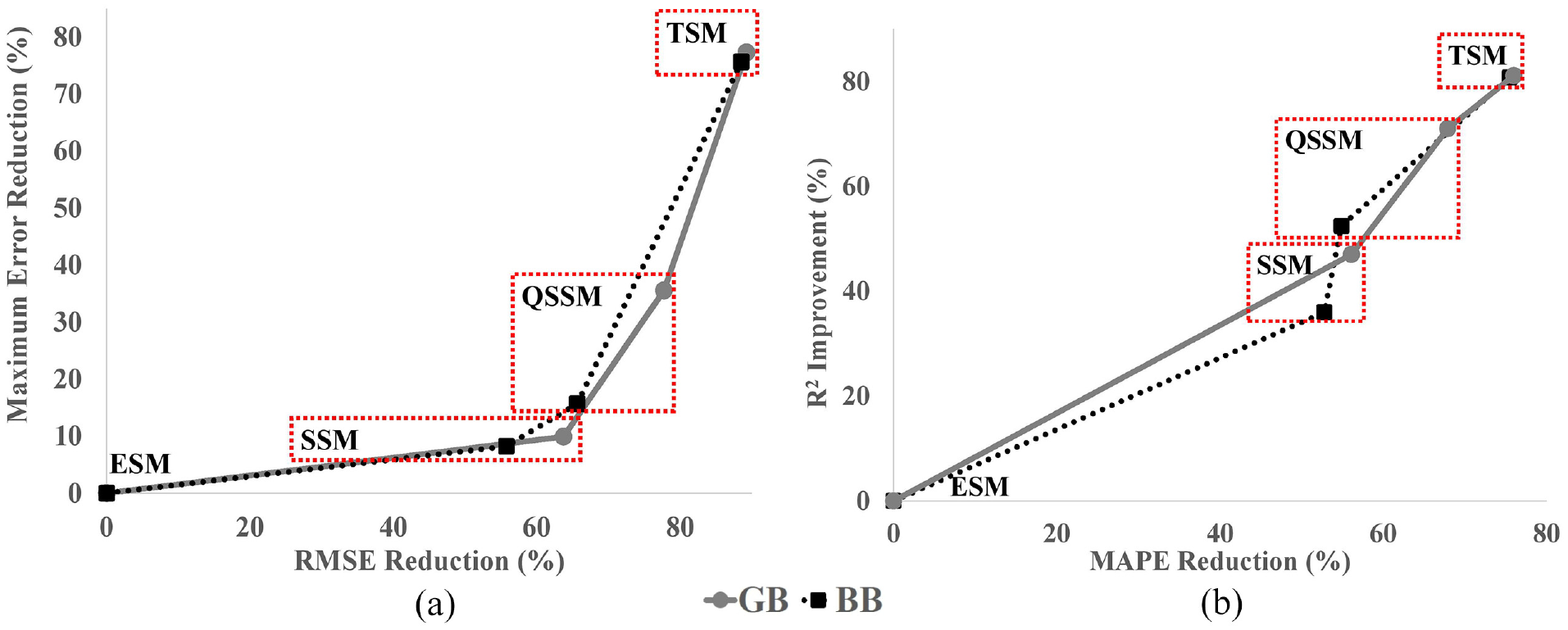
Comparison of the improvement in performance of steady-state models (SSMs), quasi steady-state models (QSSMs), and transient sequential models (TSMs) compared to engine simulation model (ESM). (a) Reduction in the maximum error and RMSE compared to ESM, (b) Reduction in MAPE and improvement in
Comparison of gray-box (GB) and black-box (BB) models, including steady-state models (SSMs), quasi steady-state models (QSSMs), and transient sequential models (TSMs) for transient and steady-state emission modeling. Modeling was carried out using IntelR XeonR CPU E3-1245 V2 @ 3.40 GHz processor and 32 GB RAM.
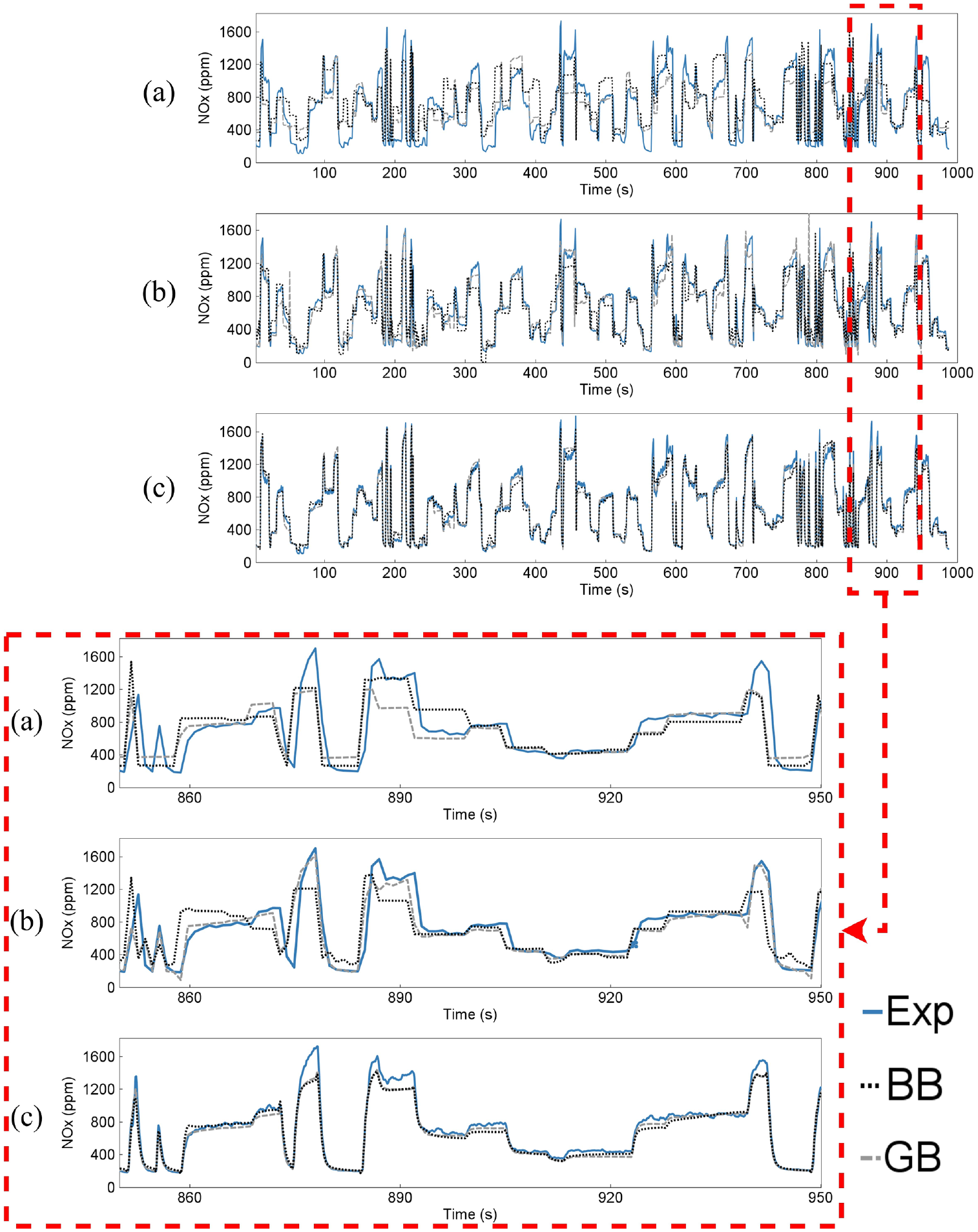
Comparison of experimental NOx emissions and predictions by black-box and gray-box models over the test data: (a) steady-state models, (b) quasi steady-state models, (c) transient sequential model (LSTM with 64 hidden neurons). The figure on the bottom displays the zoomed-in review of the region enclosed within the red box in the figure above.
Comparing the performance of these models gives a better understanding of the improvement level achieved between methodologies. The results show that, overall, the performance of the models improves as we move from left to right in Table 8 and Figure 10, and from top to bottom in Figure 11. The GB models perform better than their BB counterparts on both steady-state and transient data which can visually be seen in Figure 11. In terms of transient performance, all of the ML models outperform the ESM, with BB models being considerably faster.
Overall, the ESM has the poorest transient performance compared to all models, while BB models offer improved transient performance and faster computational speed compared to traditional physical models, making them a better choice for model-based control applications. SSMs demonstrate the best steady-state performance since these models are trained on steady-state data. Nevertheless, it is not recommended to use models trained on steady-state data for predicting transient data since SSMs perform poorly in transient situations compared to other ML methods.
In both Table 8 and Figure 10, a significant difference exists between the performance of TSMs and QSSMs, which is more pronounced than in previous studies that investigated both BB QSSMs and TSMs.21,22 The significant performance difference observed between TSMs and QSSMs in this study (Figure 10) can be attributed to the highly transient nature of the data used for modeling, as shown in Figure 4. The transient dataset used in this study involves four varying injection parameters, which contributes to the complexity of the data and highlights the need for appropriate TSM approaches to achieve accurate results. Figure 11 shows that QSSMs exhibit poorer performance in highly transient regions, where the experimental NOx emissions demonstrate more fluctuations and variations. This supports the conclusion that using time series models is essential when dealing with highly transient data, which includes high gradients of changes in engine parameters over time such as load, injection parameters, and hydrogen energy ratio. In this situation, TSMs perform much better than QSSMs. In less transient situations where changes in engine parameters over time is more gradual, QSSMs (specifically GB QSSMs) can be as accurate as TSMs.
Summary and conclusion
Predictive models for transient NOx emissions from a dual-fuel hydrogen-diesel engine using various modeling techniques and methodologies were developed. Specifically, steady-state models (SSMs), quasi steady-state models (QSSMs), and transient sequential models (TSMs) using black-box (BB) and gray-box (GB) approaches were developed. For the BB models, the machine learning (ML) model is trained solely on experimental data, with diesel and hydrogen injection timing as the inputs. For the GB models, outputs from a one dimensional (1D) engine physical model were augmented to the experimental data to train the ML model. This helped to capture the complexity of the engine’s behavior. To identify the most informative features for the GB models, two steps were performed. First, expert knowledge on NOx emissions formation in internal combustion engines (ICEs) was used to identify the most important physical model outputs. Then the four feature selection (FS) algorithms of F-test, minimum redundancy maximum relevance (MRMR), RReliefF, and least absolute shrinkage and selection operator (LASSO) were applied to further narrow down the selected features. Results showed that all of the FS algorithms outperform only expert knowledge, with the F-test algorithm yielding the best results. Using the selected features from the F-test algorithm, GB SSMs, QSSMs, and TSMs NOx models were developed. The main findings of this study are as follow:
The data-driven models, including SSMs, QSSMs, and TSMs, outperform the 1D physical engine simulation model (ESM) in transient NOx emission modeling. Furthermore, the QSSMs outperformed SSMs, and TSMs were the most accurate among the three data-driven models.
GB models outperformed BB models for all methodologies (SSMs, QSSMs, and TSMs), particularly significant improvements in SSMs and QSSMs were found. This is attributed to classical ANN used in SSMs and QSSMs do not account for the effects of previous states on the current state, while the physical model outputs in the GB models can take these effects into account. The difference in performance between GB and BB TSM models; however, is relatively small, as the time series network used in these models is already effective at capturing the effects of previous steps on the current step. Therefore, the addition of extra information provided by GB modeling may not provide significant improvements for TSMs.
The optimum number of hidden neurons in the time series layer for NOx emissions modeling using the suggested architecture in this study is between 16 and 64.
The performance difference between QSSMs and TSMs depends on the level of transience in the dataset. For highly transient datasets (for instance in this study the hydrogen energy ratio varies between 0% and 80% and there are high gradients of changes in engine parameters over time), TSMs significantly outperform QSSMs. However, for datasets with lower levels of transience, the performance gap between the two methodologies is narrower.
Both GRU and LSTM networks demonstrated strong performance in transient NOx emission modeling. Although LSTM is generally more accurate, it is also more computationally expensive. For model-based control purposes that demand real-time execution within the engine control unit (ECU) and prioritize computational efficiency, the GRU model emerges as the optimal choice. It exhibits nearly double the speed of LSTM while utilizing an equivalent number of hidden units. The BB GRU model with 64 hidden neurons, can predict transient NOx emissions with an
Potential avenues for future research include investigating
Footnotes
Appendix
Declaration of conflicting interests
The author(s) declared no potential conflicts of interest with respect to the research, authorship, and/or publication of this article.
Funding
The author(s) received no financial support for the research, authorship, and/or publication of this article.