Sage Journals: Discover world-class research

Abstract

With emissions regulations becoming increasingly restrictive and the advent of real driving emissions limits, control of engine-out NO_x emissions remains an important research topic for diesel engines. Progress in experimental engine development and computational modelling has led to the generation of a large amount of high-fidelity emissions and in-cylinder data, making it attractive to use data-driven emissions prediction and control models. While pure data-driven methods have shown robustness in NO_x prediction during steady-state engine operation, deficiencies are found under transient operation and at engine conditions far outside the training range. Therefore, physics-based, mean value models that capture cyclic-level changes in in-cylinder thermo-chemical properties appear as an attractive option for transient NO_x emissions modelling. Previous experimental studies have highlighted the existence of a very strong correlation between peak cylinder pressure and cyclic NO_x emissions. In this study, a cyclic peak pressure-based semi-empirical NO_x prediction model is developed. The model is calibrated using high-speed NO and NO₂ emissions measurements during transient engine operation and then tested under different transient operating conditions. The transient performance of the physical model is compared to that of a previously developed data-driven (artificial neural network) model, and is found to be superior, with a better dynamic response and low (<10%) errors. The results shown in this study are encouraging for the use of such models as virtual sensors for real-time emissions monitoring and as complimentary models for future physics-guided neural network development.

Keywords

Semi-empirical NOx model artificial neural networks internal combustion engines diesel transient

Introduction

The road transport sector accounts for around 16% of global greenhouse gas (mostly CO₂) emissions.¹ There has been a strong push towards powertrain electrification in the last decade in order to reduce its CO₂ footprint. However, because of its high efficiency and superior torque performance, the diesel internal combustion engine is expected to continue being an important propulsion unit, especially for heavy-duty vehicles.² Therefore, it is necessary that efforts to make its combustion clean, that is, reduce exhaust pollutant emissions, continue. A major pollutant species from diesel engines are the oxides of nitrogen (NO_x), which require substantial reduction to comply with upcoming emissions regulations.³ Moreover, with the advent of ‘real driving emissions’ (RDE) based regulations, dynamic control of NO_x emissions during transient operation has become important.

NO_x emissions from diesel engines can be managed either by controlling in-cylinder processes to lower combustion temperature (e.g. via mixture enleanment or dilution) or via exhaust after-treatment (e.g. selective catalytic reduction).¹ For dynamic NO_x control, real-time engine-out NO_x emissions data is needed to permit timely operational adjustments. Closed-loop NO_x control using exhaust sensors is impractical because such sensors are expensive and are limited by their dynamic response, which is in the order of seconds.⁴ Cyclic-level engine control requires information in the order of milliseconds. Alternatively, NO_x emissions can be predicted from engine models (so-called ‘virtual sensors’^5,6) and used for ‘model-based control’.

NO_x prediction models can be divided into three broad categories: phenomenological (also called physics-based or physical) models,^7–9 semi-empirical (or mean value) models,^10–12 and empirical models. Phenomenological models use governing equations that capture the thermochemical and fluid mechanical phenomena taking place during engine combustion and are spatially resolved (e.g. multi-zone thermodynamic or 3D CFD models^13,14). They thus have high accuracy and predictive strength (accuracy at off-design conditions) but can be computationally expensive. Empirical models use emissions look-up tables or correlations developed from engine calibration testing. They have fast response rates but perform poorly under off-design conditions. A new category of empirical models that have become popular in recent decades are so-called data-driven models. Semi-empirical models use mathematical formulations based on idealised engine combustion and NO_x production sub-models to predict general NO_x production behaviour. The resulting estimates faithfully capture trends across different engine operating conditions but are limited in their accuracy because of deviations from the ideal NO_x production mechanisms assumed. This is mitigated by calibrating the model against experimental data using tuning (or correction) factors. Semi-empirical models offer a good balance between accuracy, predictive power and computational expense, which makes them suitable for dynamic engine control.

This paper compares the transient performance of a semi-empirical NO_x prediction model to a previously developed purely data-driven model¹⁵ for a high-speed diesel engine. A brief literature survey of both the modelling frameworks is presented next.

Data-driven NO_x models

Data-driven models take advantage of the increased availability of engine performance and emissions data. They use large volumes of empirical data to ‘train’ prediction models using different machine learning techniques. Data-driven models are different from traditional empirical models in that they do not require a priori information about the process relationship, which is often prescribed through the form of mathematical correlations that are calibrated to fit experimental data. Rather, only general instructions about the input and output arguments are provided and the model uses machine learning techniques to come up with suitable structures. This makes them an enticing choice for NO_x prediction, which depends on multiple, non-linearly related engine combustion and operating parameters, including but not limited to intake air properties, injection settings, trapped mixture composition (air-fuel ratio, internal and external EGR) and mixedness levels. In recent years, such emission models have gained significant interest within the engine development community. A variety of machine learning techniques have been used within the community including gradient boosting techniques,¹⁶ random forests¹⁷ and physics aware machine learning techniques.¹⁸ The machine learning implementation approach of Artificial Neural Networks (ANN) also referred to as deep learning or simply neural networks has been a predictive tool of choice for engine researchers because of its suitability for modelling complex, non-linear processes of the sort that take place during combustion.¹⁹ ANN models capture non-linear effects through the activation function linking neurons in the hidden and output layers.

Various studies have used the artificial neural networks approach for the prediction of engine performances and emissions. Parlak et al.²⁰ demonstrated their ANN model in predicting specific fuel consumption and exhaust temperature with fast and consistent results featuring a low absolute relative error compared to the experiment. Fang et al.²¹ highlighted the importance of ANN input feature selection where the ANN with Pearson correlation selected features demonstrated improved prediction in the low-NO_x region. Applying the same model structure, Fang et al.¹⁵ further extended the ANN model to predict cyclic transient NO_x emissions. While the model was able to capture the critical correlation of in-cylinder peak pressure in transient NO_x formation in both transient load step-up and step-down, a deviation was observed for all tested load step-down conditions suggesting additional experimental data and/or details of the underlying physical phenomena need to be included under these conditions. This is the baseline ANN model used in the current work. Similarly, the model constructed by Di Mauro et al.¹⁹ was found to be able to predict the indicated mean effective pressure (IMEP) and its coefficient of variation (CoV) in a spark-ignited internal combustion engine discovering a strong correlation between the modelled CoV and the experiments. However, a systematic overprediction of CoV was observed for low CoVs while higher CoVs were underpredicted by the ANN model suggesting missing physical parameters for the ANN input features. More recently in order to overcome some of the above-mentioned challenges, super learner-based ensemble machine learning approaches were developed for rapid engine design optimisation targeting better fuel efficiency and lower emissions^22–24

From the above-mentioned studies, the success of data-driven models is found to rely on high-fidelity training data where the optimised models are found fast and precise, particularly within the training domain. However, it was also indicated that such models can have reduced responses to physical changes in the system especially when the changes occur outside the training domain or when the model is trained using steady-state data.

Semi-empirical NO_x models

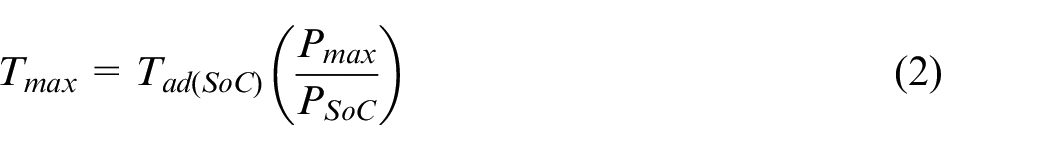
Simplified chemical kinetics based semi-empirical models are computationally inexpensive and with some initial tuning, can yield accurate NO_x predictions across a wide range of operating conditions.¹⁰ These models commonly assume that NO production takes place predominantly in the mixing-controlled (diffusion) combustion phase and that the major production pathway is the thermal (Zeldovich) mechanism.^25,26 Crank-angle resolved cylinder-pressure is used to determine the thermal state of the combustion mixture and the characteristic thermal NO production temperature.^7,10,12 Adiabatic flame temperature $(T_{ad})$ is commonly used as the characteristic NO production temperature^7,10,27 as it is considered to be a good estimate of the NO production temperature of a quasi-steady diffusion flame.^12,26 Because cylinder pressure sensors are expensive and not found in production engines, some semi-empirical models estimate the cylinder pressure indirectly from fuel injection data.^28,29

NO₂ can form a significant (up to 30%³⁰) fraction of the total engine-out NO_x emissions from diesel engines, particularly at higher levels of EGR, but to avoid increasing model complexity, semi-empirical models usually do not explicitly estimate NO₂. They assume that NO₂ emissions are either negligible or proportional to NO emissions, which can be reconciled during model calibration using experimental NO_x data. Some semi-empirical models, however, have additional mechanisms to estimate NO₂.^29,30

Semi-empirical models are typically calibrated using steady-state engine data (static tuning) and then their performance is tested at other steady-state points^7,11,12; or for models being developed for real driving / transient control, additional testing is conducted over different driving cycles. If needed, this is followed by dynamic model tuning using NO_x emissions data collected from on-board or portable emissions analysers.^28,29,31,32 Such real driving NO_x emission sensors, however, can be limited by their measurement accuracy (10%–12% errors^6,29).

Lyons and Timoney¹⁰ used the simplified Zeldovich mechanism with $T_{ad}$ to estimate NO_x emissions. Then using a quadratic formulation, they estimated actual NO_x emissions by regressively fitting the predictions to measured values from 521 steady-state test points. They reported good model performance (R² over 98%). Arrégle et al.²⁷ assumed that NO production was proportional to the instantaneous apparent heat release rate (AHRR). The model did not explicitly estimate Zeldovich NO but, instead, used $T_{ad}$ , AHRR and engine speed in an exponential NO_x production equation. Engine speed served as a proxy for in-cylinder mixing and turbulence levels. Three tuning parameters were calibrated using a fitting algorithm. Guardiola et al.¹² modified the Arrégle et al. model by additionally accounting for ‘re-burning’ (the re-entrainment of NO in the reducing zone of a diffusion flame), which improved the prediction accuracy by 1.3% at a slight computational time penalty.

Park et al.⁷ used CFD simulated NO production results at 35 different steady-state operating conditions to develop a physical model. The model used $T_{ad}$ and an effective NO production window to compute cyclic NO emissions. It had only one tuning parameter (Zeldovich pre-exponential coefficient) and reported overall good performance (R² over 98%). Guardiola et al.³¹ used an exponential NO_x correlation with multiple correction factors (for inlet air temperature and humidity, coolant temperature and transient operation) to predict emissions during transient operation. The ‘nominal’ NO_x values, instead of being estimated from a Zeldovich-derived equation, were obtained from steady-state experimental calibration maps. The model produced an average error of 50 ppm during transient operation. Barbier et al.³² used real driving NO_x data from a hybrid diesel vehicle to calibrate the Guardiola et al.³¹ model, and reported mean absolute errors of around 20 ppm. They declared real driving NO_x emissions to be a ‘viable’ method of calibrating semi-empirical NO_x models. Lee et al.²⁹ in their semi-empirical model, assumed that NO formation was proportional to the amount of fuel injected and reported around 10% error in transient driving NO_x predictions.

Paper scope

The current study uses a modified version of the semi-empirical model by Part et al.⁷ to test the hypothesis that a physical model that uses peak cyclically-resolved cylinder pressure to predict cyclic NO_x emissions will have good transient performance. This hypothesis is based on high-speed (cyclic) NO_x emissions measurement studies that have reported strong linear correlations between peak cylinder pressure and NO_x emissions.^21,33–35 The modified physical model instead of using CFD-predicted cylinder pressure uses experimental cylinder pressure data for 1800 consecutive cycles with cyclic, transient exhaust NO_x data (measured using advanced ‘fast’ NO and NO₂ analysers) for model development and testing. Moreover, it directly computes thermochemical properties of the combustion mixture using the open source chemical-kinetics and equilibrium solver Cantera,³⁶ instead of using correlations developed for a limited range of mixture conditions.

The paper also presents an alternate (to using portable or on-board NO_x sensors) means of testing and dynamically tuning semi-empirical transient NO_x prediction models by using high accuracy fast exhaust NO_x measurements.

Methodology

Experimental setup

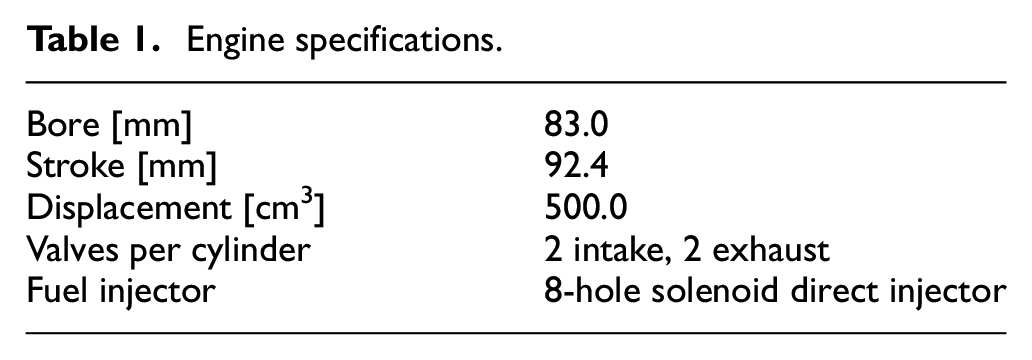
Experimental data was collected from a single-cylinder, automotive-type, compression-ignition (diesel) research engine. The engine and the test setup have been described in detail in previous publications.^21,37 Important specifications of the engine are summarised in Table 1 and a schematic of the setup with relevant sensors is shown in Figure 1.

Table 1.

Engine specifications.

Bore [mm]	83.0
Stroke [mm]	92.4
Displacement [cm³]	500.0
Valves per cylinder	2 intake, 2 exhaust
Fuel injector	8-hole solenoid direct injector

Figure 1.

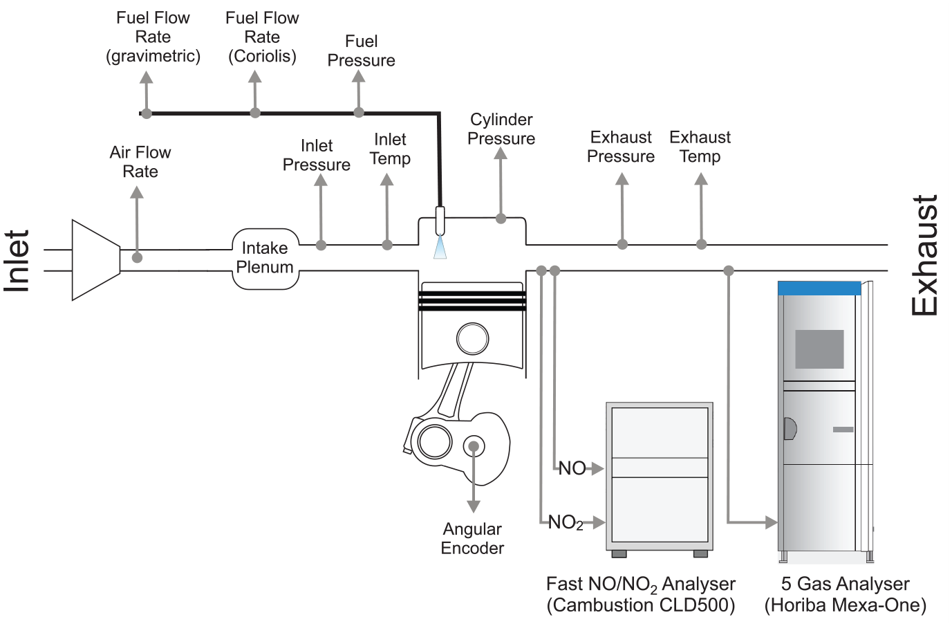
Schematic of experimental setup with relevant sensors labelled.

Cylinder pressure was measured every 0.1 CA° using a Kistler 6046Asp-3-2 transducer, and air and fuel flow rates were recorded at 1 Hz. A Sierra CP Airtrak 620S flow sensor was used for air flow measurement and fuel flow was measured independently using a gravimetric (Sierra CP FuelTrak) and Coriolis (Siemens MASS2100) flow meter. The engine was run on a standard EN590 compliant diesel fuel.

Exhaust NO_x emissions were measured using a standard (‘slow’) Horiba MEXA-ONE analyser, and ‘fast’ NO and NO₂ analysers manufactured by Cambustion. The Horiba MEXA-ONE worked on the chemiluminescence principle to measure NO and NO_x concentrations. Its NO channel had a response time of 1.2 s while the NO_x channel had a response time of 1.5 s. 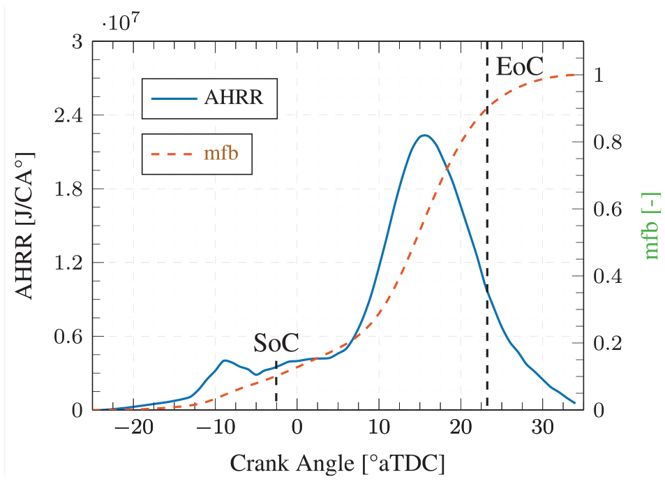However, because of transport delays due to the exhaust sampling point being significantly downstream of the exhaust ports (after an exhaust backpressure valve and a smoothing tank), the effective response time for the analyser was 15 s.³⁷ The fast NO analyser (Cambustion CLD500) also worked on the chemiluminescence principle but used a constant pressure heated sampling chamber to have a low $T_{10 - 90 %}$ response time 0.2 ms. The fast NO₂ analyser used laser-induced fluorescence with a heated capillary gas sampling system to achieve a high response rate of $T_{10 - 90 %}$ = 0.2 ms.³⁸ Exhaust samples for the fast NO_x analysers were collected approximately 70 mm downstream of the exhaust port. Special care was taken to ensure that measurement errors were kept low, including recalibrating the fast NO_x analysers every hour to account for any calibration drift. The raw signals from the fast NO analyser were also corrected for any quenching that could have occurred in the chemiluminescence detector.³⁷

As discussed in Fang et al.,¹⁵ slow and high speed data, which were recorded every 1 s and 0.1 CA°, respectively, were time-aligned to account for transportation delays. Crank-angle resolved NO_x data was used to calculate cyclic NO_x emissions by averaging NO_x concentration during the exhaust valve open period. Figure 2 shows sample NO_x results from the fast analyser for three consecutive cycles, along with corresponding cylinder pressure data to illustrate the NO_x averaging window from exhaust valve opening (EVO) to exhaust valve closing (EVC). This period was selected as the fast NO_x signals are valid only during this period when combustion products from the cylinder are being expelled. A mean value is then calculated over the valve opening period which represents NOx emissions for that cycle. Ball et al.³⁹ used a similar averaging approach and reported close (greater than 95% for most cases) agreement with mass averaged high speed NO measurements.

Figure 2.

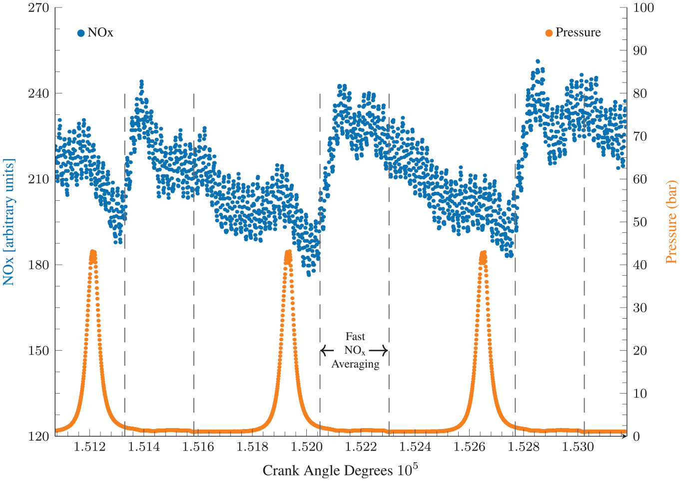
Crank angle resolved fast NO_x data and the corresponding crank angle resolved pressure measurements. Sample crank angle resolved NO_x averaging windows from EVO to EVC (dashed) for cyclic NO_x calculations.

Owing to data confidentiality requirements, all emissions data reported here has been re-scaled by an arbitrary scaling factor and thus presented in ‘arbitrary units’.

Operating conditions

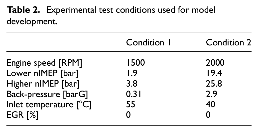
Data from two transient engine operating conditions, summarised in Table 2, was used for model calibration and testing. Transient engine operation was achieved on the engine dynamometer by adjusting fuel injection duration to switch between low and high load operating points, whilst maintaining other combustion parameters such as location of 50% mass fraction burned constant. High and low speed data were continuously collected for at least 1800 cycles at each condition. The first operating condition (Condition 1) represents low-load, medium-speed transient operation while Condition 2 represents high-load, high-speed transient operation. For both operating conditions, alternation load steps are applied to represent real driving conditions.

Table 2.

Experimental test conditions used for model development.

	Condition 1	Condition 2
Engine speed [RPM]	1500	2000
Lower nIMEP [bar]	1.9	19.4
Higher nIMEP [bar]	3.8	25.8
Back-pressure [barG]	0.31	2.9
Inlet temperature [°C]	55	40
EGR [%]	0	0

Physical model

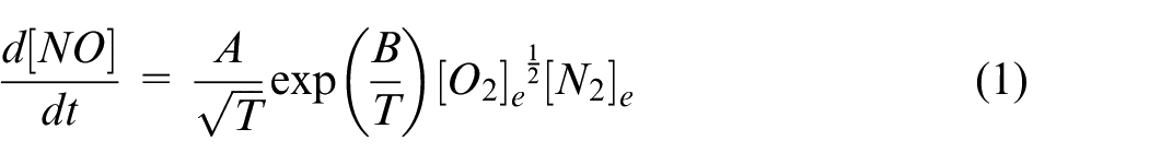
A physical model was adapted from the model of Park et al. ⁷ The model assumed that NO was produced only during diffusion combustion and was formed via the thermal (Zeldovich) pathway, which is active at temperatures above 1800 K.⁴⁰ The simplified thermal NO production rate equation, equation (1),²⁵ which is based on steady-state and equilibrium assumptions applied to the extended Zeldovich mechanism (Reactions R1 to R3) was used. In equation (1), T is the absolute temperature, terms within square brackets are molar concentrations, subscript e denotes equilibrium concentrations, A is an empirical pre-exponential factor, and B is an activation energy index.

\frac{d [N O]}{d t} = \frac{A}{\sqrt{T}} \exp (\frac{B}{T}) {[O_{2}]}_{e}^{\frac{1}{2}} {[N_{2}]}_{e}

(1)

O + N_{2} = NO + N

(R1)

N + O_{2} = NO + O

(R2)

N + OH = NO + H

(R3)

Peak thermal NO production rates were used as a proxy for average NO production rates as both were found to be proportional by Park et al.⁷ Crank-angle resolved measured cylinder pressure, along with calculated trapped cylinder mass and volume, were used to determine average cylinder temperature. Trapped cylinder mass was calculated from measured air and fuel flow rates by assuming a constant residual gas fraction, which represents the fraction of gases retained from the preceding cycle, that is, ‘internal EGR’.

For our study, $T_{ad}$ (adiabatic flame temperature) was assumed to be the characteristic NO production temperature and was calculated at the start of combustion (SoC), taken to be the 10% mass fraction burned (mfb) point, using Cantera. N-heptane was selected as the single component chemical surrogate to represent the diesel fuel. A constant-volume batch reactor was used to simulate $T_{ad}$ in Cantera where a 68-species skeletal mechanism from Lu et al. for n-heptane is used.⁴¹ Then the temperature at the peak pressure point $(T_{\max})$ was calculated using equation (2) by assuming that the burned gas was compressed isentropically during combustion. $T_{\max}$ was computed for each cycle and was used to calculate the peak cyclic NO production rate from equation (1). Equilibrium O₂ and N₂ concentrations were also obtained from Cantera.

T_{\max} = T_{ad (SoC)} (\frac{P_{\max}}{P_{SoC}})

(2)

Cyclic NO emissions were then calculated using the peak NO production rate and an effective NO production period of 10%–90% mfb illustrated in Figure 3. Since the highest NO production rates in diesel flames have been observed in the stoichiometric regions,²⁶ an equivalence ratio $(ϕ)$ of 1 was used for thermal NO production calculations.

Figure 3.

Combustion and effective NO_x production windows for a selected cycle.

NO_x estimates were obtained from the NO predictions by assuming a constant NO₂:NO_x ratio. From the high-speed NO and NO₂ measurements averaged for all the recorded cycles, conditions 1 and 2 had NO₂:NO_x ratios of 0% and 10%, respectively, which were used in the physical model. The high NO₂:NO_x at condition 2 are believed to result from the sporadic phenomenon of ‘injector dribble’ which was more active at the high load condition. Hydrocarbons introduced to the reacting mixture by injector dribble can generate HO₂ radicals and oxidise some of the NO to NO₂ as per Reaction R4. This was investigated in previous studies on the same engine using high-speed exhaust NO, NO₂ and hydrocarbon sensors.^35,38 A strong, linear correlation $(R^{2} > 0.8)$ between cyclic exhaust hydrocarbon and NO₂ was observed under similar conditions.

NO + {HO}_{2} = {NO}_{2} + OH

(R4)

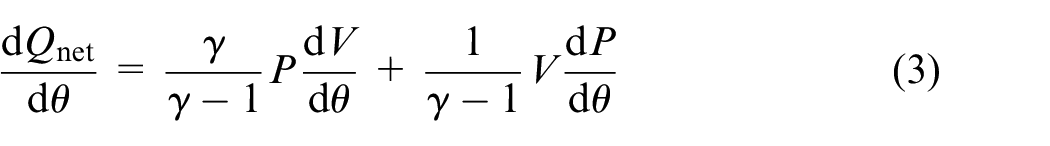
A simple net apparent heat release formulation shown in equation (3) that assumed a constant ratio of specific heats $(γ)$ was used to determine the mfb profile.²⁵ Guardiola et al.¹² showed that using a more comprehensive AHRR model increased computational time by more than 200 fold. Therefore the choice of the simple AHRR model was considered appropriate.

\frac{d Q_{net}}{d θ} = \frac{γ}{γ - 1} P \frac{d V}{d θ} + \frac{1}{γ - 1} V \frac{d P}{d θ}

(3)

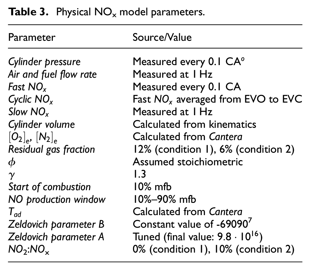
The model’s architecture is summarised in Figure 4 and a summary of the important parameters used in it and their sources is provided in Table 3.

Table 3.

Physical NO_x model parameters.

Parameter	Source/Value
Cylinder pressure	Measured every 0.1 CA°
Air and fuel flow rate	Measured at 1 Hz
Fast $N O_{x}$	Measured every 0.1 CA
Cyclic $N O_{x}$	Fast $N O_{x}$ averaged from EVO to EVC
Slow $N O_{x}$	Measured at 1 Hz
Cylinder volume	Calculated from kinematics
$[O_{2}]_{e}$ , $[N_{2}]_{e}$	Calculated from Cantera
Residual gas fraction	12% (condition 1), 6% (condition 2)
$ϕ$	Assumed stoichiometric
$γ$	1.3
Start of combustion	10% mfb
NO production window	10%–90% mfb
$T_{ad}$	Calculated from Cantera
Zeldovich parameter B	Constant value of -69090⁷
Zeldovich parameter A	Tuned (final value: $9.8 \cdot 10^{16}$ )
NO ₂:NO_x	0% (condition 1), 10% (condition 2)

Figure 4.

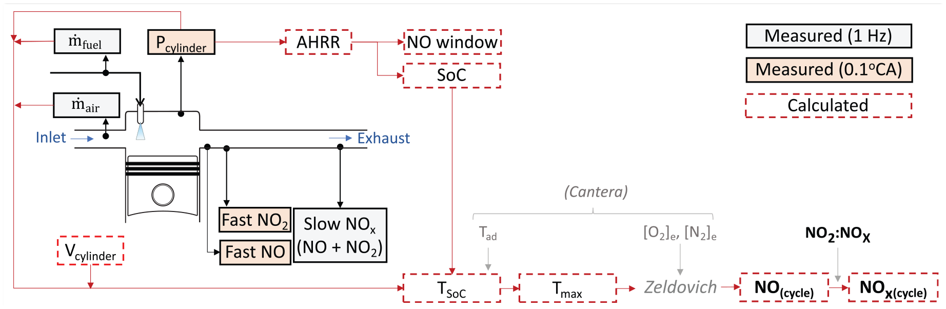
Overview of the physical NO_x model’s architecture.

Neural network model

The artificial neural network model used for comparison has been described in detail in previous publications.^15,21 It was based on a common ANN structure known as a multilayer perceptron illustrated in Figure 5, and comprised one input layer, one hidden and one output layer. The input parameters were carefully chosen through different filtering approaches where 14 engine parameters were identified and used as the input layer. A log-sigmoid activation function with a mean squared error (MSE) based error function was used. While the use of multiple-layer structure is adapted in a lot of studies centring around NO_x prediction, for the conditions tested in this study one-layer structure showed very high accuracy for all conditions tested. It is to be noted that the conditions studied here were never used or included in both the training and validation processes during the construction of the neural network. In addition, no fast NO_x results and maximum cyclic pressure were ever used during the training of the neural network. The neural network training was purely based on steady-state slow NO_x data. The predictions from ANN demonstrated in this study as a comparison therefore are mostly based on extrapolation where cyclic maximum pressure and other 13 channels of repopulated data are together used as the input. It is to be noted that the emphasis of this study is not on the machine learning aspect, but rather on the development of the semi-empirical NOx model, which holds greater relevance in this context. Nevertheless, we believe it is important to include previous results of a simplified machine learning model, considering it was trained using the same dataset. While the prior paper on machine learning primarily dealt with the impact of engine parameter selection, rather than the development of the ANN model itself, its inclusion in this study is justified. Both the semi-empirical and the machine learning models utilised maximum cylinder pressure as a key factor. This also motivates us to pursue a more physics-based approach in future machine learning model development. We also acknowledge the recent advances in ML modelling in the context of engine development which can significantly improve the current neural network model. For example, the use of hyperparameter tuning and optimization⁴² and the use of superlearner-based ensemble-ANN techniques^23,24 can be of interest.

Figure 5.

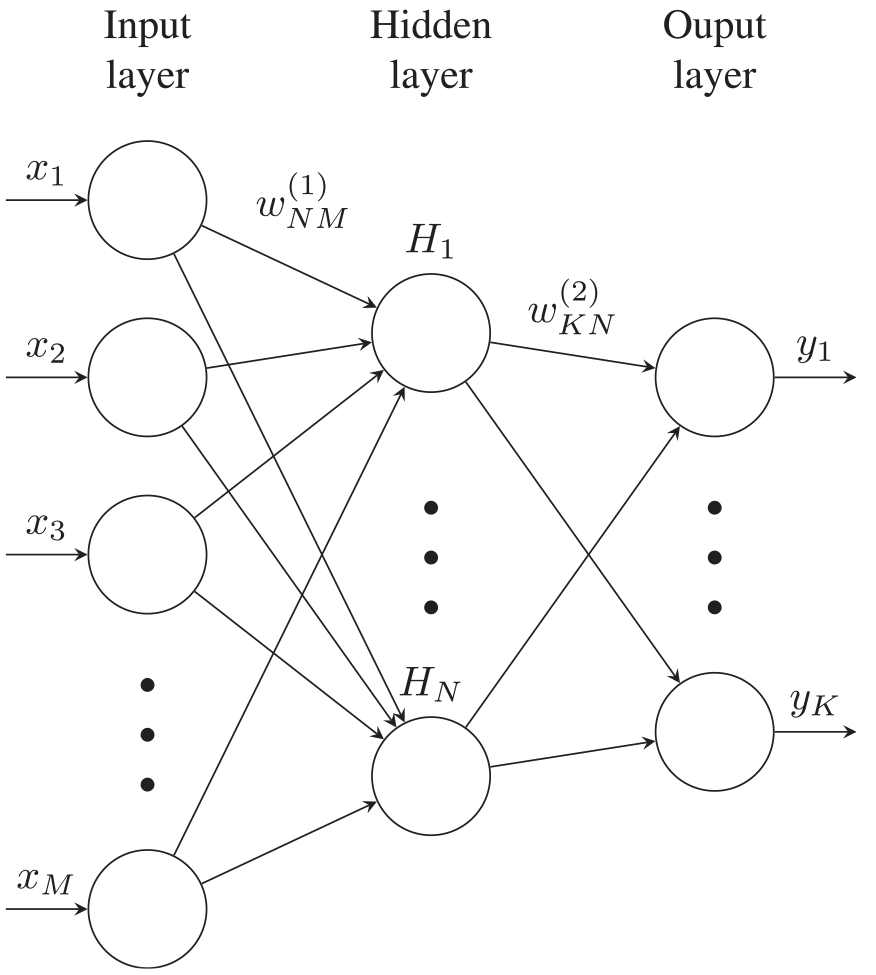
Schematic diagram of the neural network structure used as comparison.

Results and discussion

Physical model calibration and testing

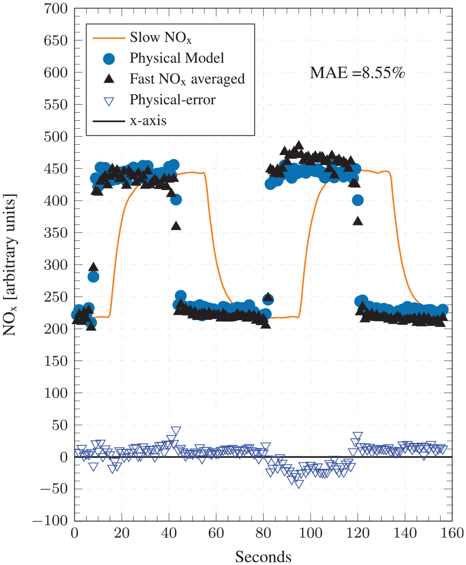
The model was calibrated manually for condition 1 by comparing cyclic experimental and physical model-predicted NO_x concentrations. This entailed selecting physically reasonable values for the Zeldovich coefficient A and an effective SoC timing that minimised NO_x prediction errors. It was found during calibration that using slightly higher $P_{SoC}$ values to find $T_{\max}$ in equation (2) yielded more accurate results. Therefore, cylinder pressure slightly after 10% mfb was used as a marker for effective SoC. An effective SoC of 17.5% mfb was used in the tuned model.

Figure 6 compares the physical model predictions with experimental values at condition 1 for the 1800 cycles considered. It also reports the cyclic errors (at the bottom) and the mean absolute error (MAE) as a percentage. Predictions from the ANN model, which will be discussed later, are also shown. The physical model demonstrates very good accuracy and transient response, whereby a low MAE of 8.55% is registered and the NO predictions track experimental values closely during the highly transient step-up/down events. Figure 7 illustrates the accuracy of the physical model on a correlation plot and reports a high goodness of fit with a coefficient of determination (R²) value of 0.95. 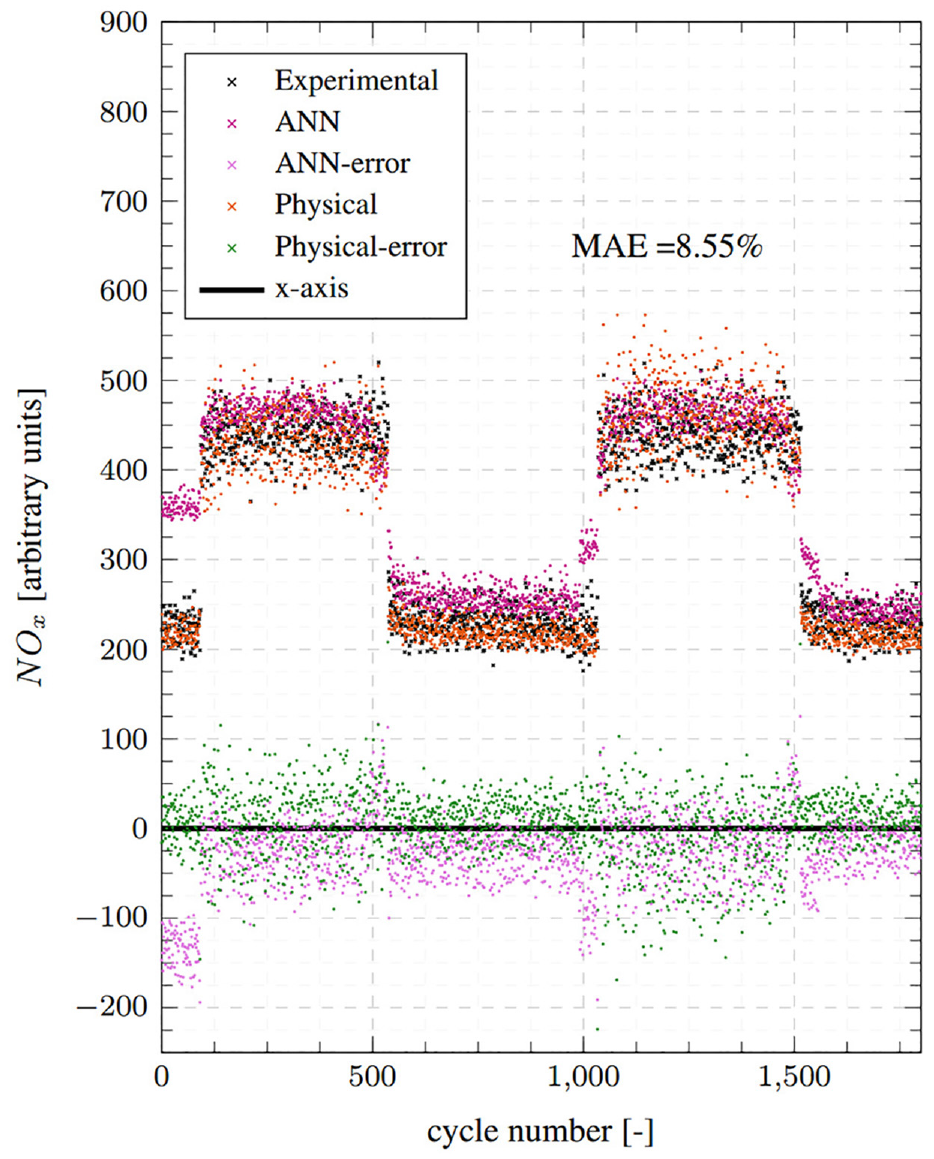No prominent data clusters are observed away from the $y = x$ line. These results are encouraging as they demonstrate that a simple physical model with minimal tuning can capture cyclic level changes in NO_x emissions.

Figure 6.

Top: Test point 1 comparisons between the physical model predictions, ANN NO_x model predictions and the cycle averaged fast-NO_x analyser readings. Bottom: Absolute errors for both ANN and physical models.

Figure 7.

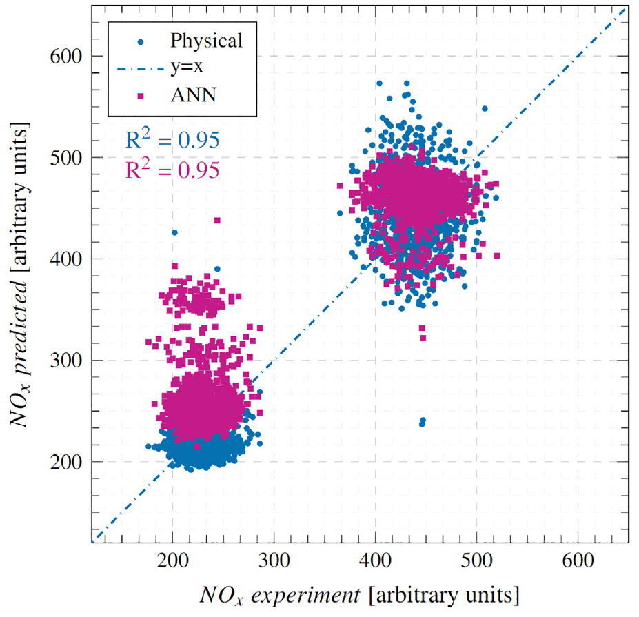
Correlation between experimental and predicted NO_x emissions at condition 1.

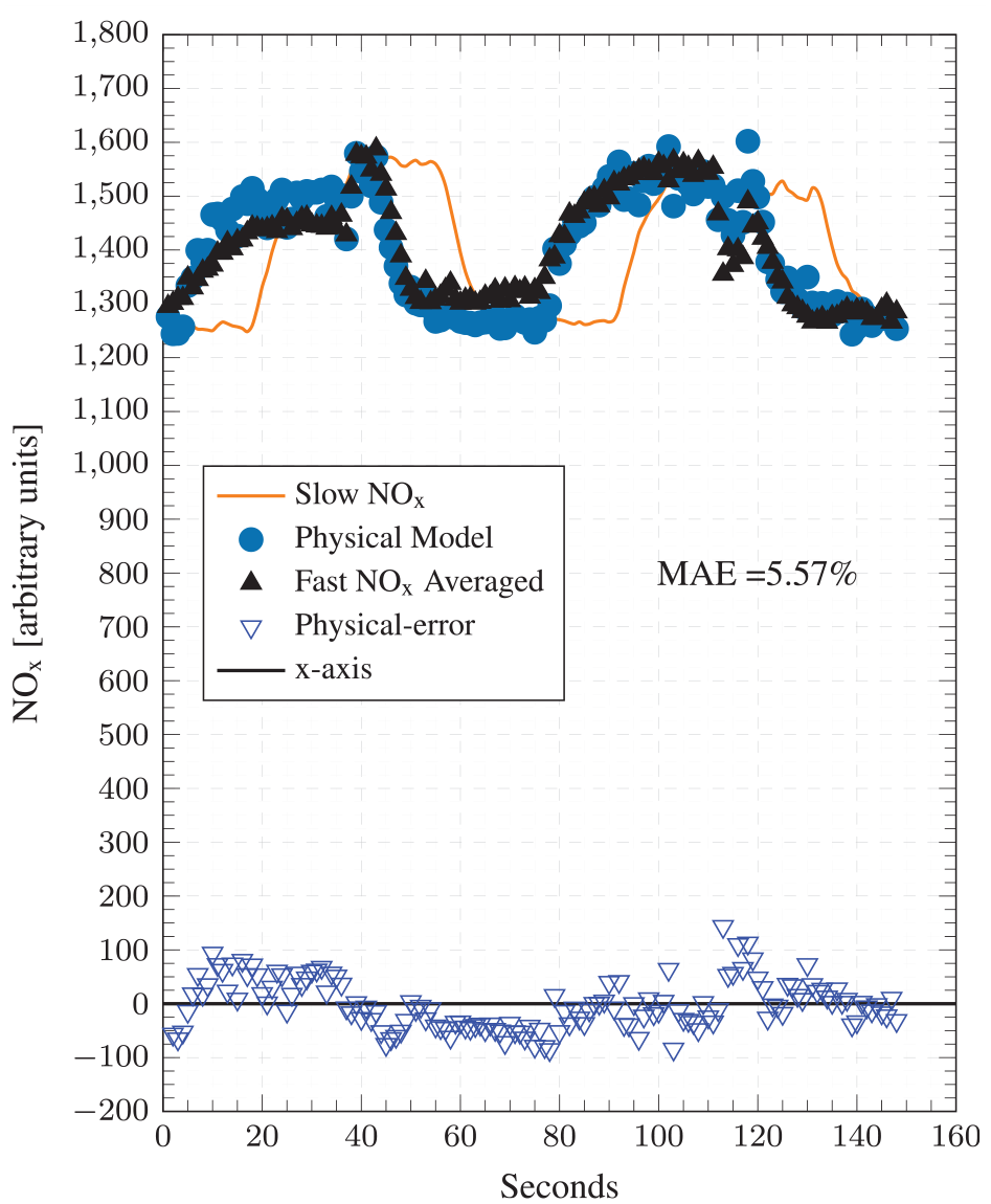
Next, the calibrated model was tested at condition 2 without changing any parameter settings except for the residual gas fraction, which was halved from 12% to 6% – assuming that the higher load case would have lower trapped residuals.²⁵ Model prediction results at this condition are presented in Figure 8. The model registers a very good transient performance by closely tracking experimental NO_x values and rapidly responding to load changes. The resulting errors are low with an MAE of 5.57%. The model’s performance at condition 2, which represents high load transient operation, is very encouraging for transient NO_x monitoring and control as the model was tuned under significantly different operating conditions at condition 1.

Figure 8.

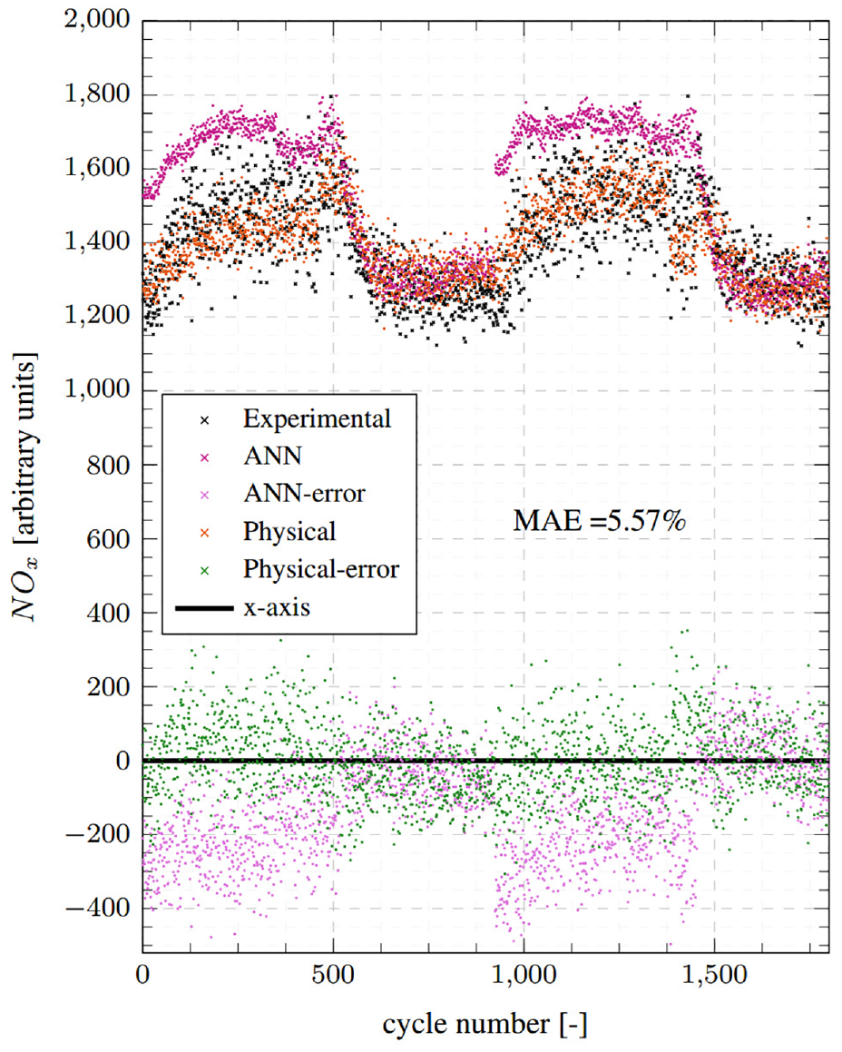
Top: Test point 2 comparisons between the physical model predictions, ANN NO_x model predictions, and the cycle averaged fast-NO_x analyser readings. Bottom: Absolute errors for both ANN and physical models.

Figure 9 presents the model’s prediction results at condition 2 as a correlation plot. A strong correlation between predicted and experimental NO_x emissions with an R² of 0.70 is observed. As with condition 1, no obvious clusters away from the $y = x$ line are present, which showcases the model’s predictive strength across the entire load range swept at condition 2. However, the R² value is lower than that at condition 1 (0.95), signifying a larger spread in the prediction results. This is an artefact of the experimental NO_x data at condition 2 having a higher degree of scatter. The absence of two distinct high and low load clusters in Figure 9, which were observed in Figure 7 for condition 1, illustrates this increased scatter. The high experimental scatter is primarily due to the transient load step at condition 2 being an increase of around 33% whereas at Condition 1 the increase is 100%. In addition at condition 2, some of the scatter can be attributed to the conversion of some of the NO produced during combustion to NO₂ via injector dribble-induced reactions discussed earlier.³⁸ At the relatively high load of condition 2, it is unlikely that much thermal NO₂ will be being produced and so this hydrocarbon induced mechanism is a likely cause.

Figure 9.

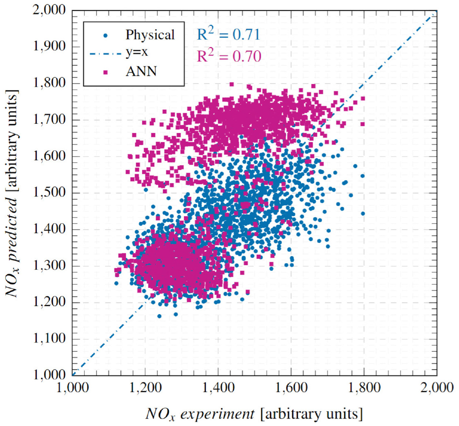
Correlation between experimental and predicted NO_x emissions at condition 2.

The accuracy of the physical model’s predictions is affected as a result because it only considers thermally produced NO and ignores other NO production and conversion mechanisms. The addition of sub-models for non-thermal NO_x production can potentially improve the results. This limitation of the model can, however, be leveraged for diagnostic purposes to identify abnormal NO_x production activity or sensor malfunction when scatter in NO_x estimates increases.

Comparison with ANN model

The performance of the physical and the ANN models is compared by referring to the results presented above in Figures 6 to 9. Overall, the physical model is found to perform better than the ANN model, both in terms of transient and steady-state accuracy as evidenced by the consistently low error values in Figures 6 and 8. The physical model has MAEs of 8.55% and 5.57% for conditions 1 and 2, respectively, while the ANN model has errors of 12.69% and 10%. Moreover, as was highlighted in Fang et al.¹⁵ and can be seen from the ANN results reproduced here, the ANN model has regions of high errors during transient operation, especially during step-up events, for example, first 100 cycles of condition 1 and cycles around 1000 when the second step-up event takes place (Figure 6); and first 400 cycles and cycles 9000-1500 for condition 2 (Figure 8). These high error points in the ANN model estimates appear as clusters in the corresponding correlation plots (Figures 7 and 9) above the $y = x$ line, signifying overestimation errors. The clustering observed in the ANN results is an artefact of its architecture and training regime, whereby steady-state data was used for its training. As mentioned earlier, the 14 input parameters used as input channels for the ANN model are repopulated with only cyclic maximum pressure used at the same frequency as the NO_x experiment, which can significantly contribute to poor predictions near load steps. This is further confirmed at steady regions of both operating conditions where the ANN model performed better for both conditions. It is to be noted that Condition 2 by nature can be significantly more challenging for the neural network model based on steady-state data, due to the different response times of all input channels and the fast condition changes that occurred in the testing. During high-load conditions, the discrepancies are also likely due to the fast analyser picking up the cycle-to-cycle variations which the model is not trained with. Whereas the physical models relying on cyclic peak pressure can also reflect this cycle-to-cyle variation. This was highlighted previously in our previous study.¹⁵ This further highlighted the importance of having high-frequency high-fidelity data as an input for neural network-based models which can be seen as a challenge in using such models for cyclic NO_x predictions.

The reason for the physical model’s superior response is its structure where crank angle resolved cylinder pressure data was used to capture cyclic changes in combustion intensity and phasing, and its effects on the NO production temperature. Previous high-speed NO_x measurement studies^33–35 have reported strong linear correlations between peak cylinder pressure and NO_x emissions. Fang et al.²¹ performed the Pearson correlation test on 32 measured engine parameters and cyclic NO_x emissions; and identified peak cylinder pressure as the parameter with the highest importance. They also reported a high Pearson correlation coefficient score for coolant temperature change. This indirectly pointed to a strong correlation between peak cylinder temperature and NO_x emissions because an increase in peak cylinder temperature leads to increased wall heat transfer and coolant temperature changes.

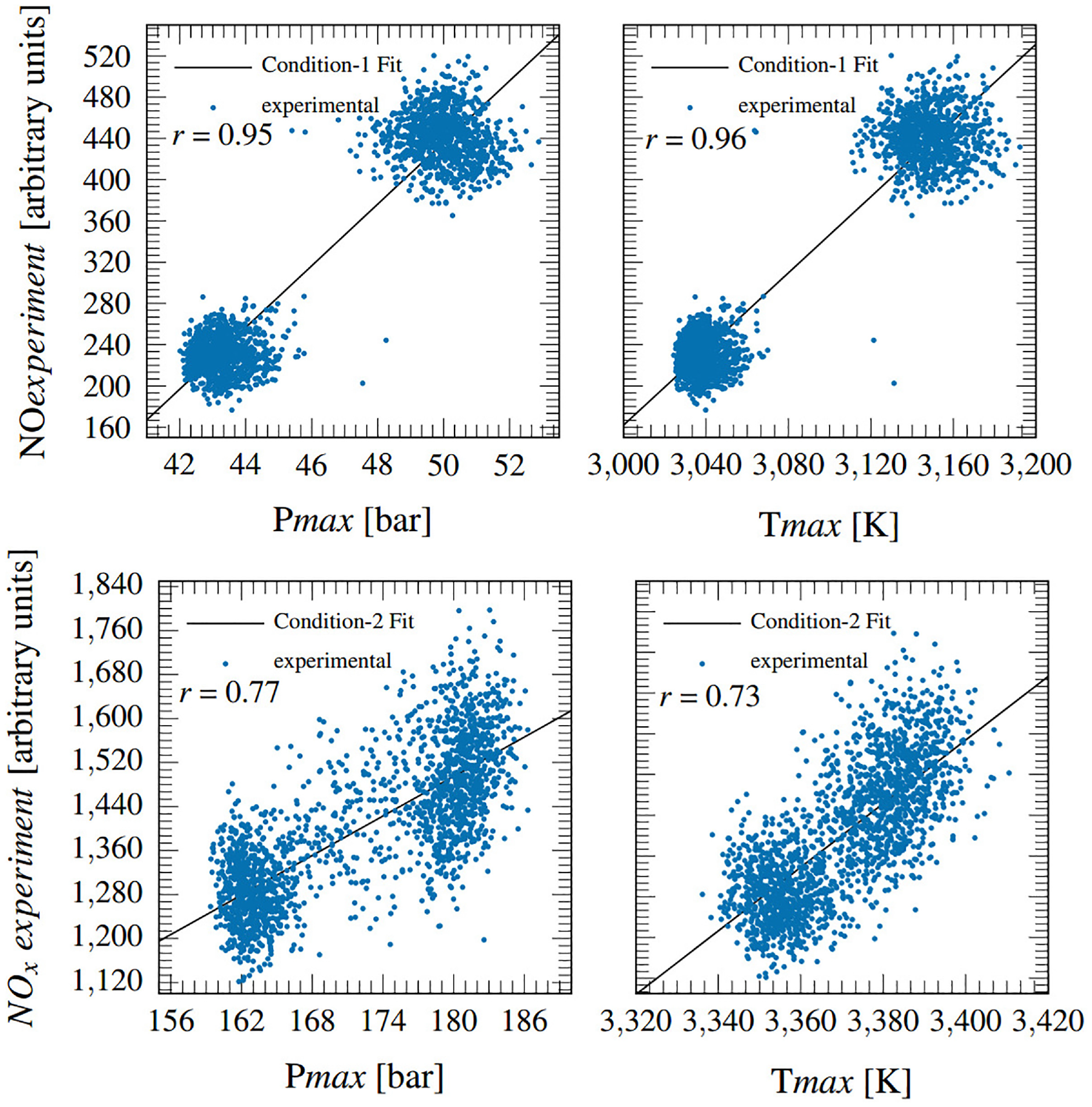
These findings are confirmed for the current data set in Figure 10 in which the left column shows the strong correlation that exists between peak pressure (measured) and exhaust NO_x; and the right column shows a comparably strong correlation between $T_{\max}$ (calculated from the physical model) and cyclic NO_x emissions. This also demonstrates the suitability of the characteristic $T_{ad}$ based NO_x production temperature choice. It is worth noting that the predicted value correlation with the experimental NO_x follows the correlation highlighted in Figure 10 where Condition 1 is significantly better. This is again likely caused by injector dribble-induced reactions during the experiments.

Figure 10.

Correlation of experimental cyclic NO_x with (left) peak cylinder pressure and (right) corresponding cylinder temperature.

The observed strong correlation between in-cylinder peak thermal conditions and exhaust NO_x concentrations can serve as a guide for developing simple (data-driven or physics-based) NO_x prediction models by establishing accurate estimation of peak cylinder pressure and temperature as a requirement for accurate NO_x predictions; and data from advanced fast NO_x analysers (like the ones used here) can provide cyclic level information about changes in NO_x emissions for dynamically tuning such models. Since the ANN model was not trained using cyclic data, it failed to accurately predict peak cylinder pressure during transient operational changes and thus had high errors during those periods as seen in Figures 6 and 8.

Comparison with slow speed NO_x

The slow-speed, chemiluminescence based NO_x analyser is commonly considered the benchmark for measurement accuracy but its slow dynamic response limits its utility for accurately measuring transient NO_x emissions. Therefore on-board and portable emissions analysers, which have higher measurement errors, have been used for developing transient NO_x models.^28,29,31,32 It has been shown previously³⁷ that measurements from fast NO_x analysers are in very close agreement with those from slow-speed analysers, which provides confidence in their measurement accuracy and thus makes them a source of high-fidelity transient NO_x data.

Figures 11 and 12 compare the experimental and predicted cyclic NO_x (averaged over 1 s windows) to the slow speed measurements. The cyclic averaged NO_x measurements are carefully aligned with the slow speed measurements through other channels to ensure a fair comparison. It can be seen that step responses in the slow speed analyser readings are severely delayed, which significantly under or over-reports exhaust NO_x concentrations during step-up and step-down episodes, respectively. This is linked to the physical position of the slow analyser further downstream in the exhaust, and the slower rise and drop are caused by the its slower dynamic response ( $T_{10 - 90 %}$ of 1.5 s vs 0.2 ms). The difference in peak NO_x emissions between two analysers is also likely caused by the location of the analyser where the agreement between the two analysers is highlighted in previous experimental work assuring the fidelity of both measurements.³⁵

Figure 11.

Test point 1 comparisons between the cycle averaged physical NO_x model predictions, the time-averaged fast-NO_x analyser readings and the slow-NO_x analyser readings.

Figure 12.

Test point 2 comparisons between the cycle averaged physical NO_x model predictions, the time-averaged fast-NO_x analyser readings and the slow-NO_x analyser readings.

The physical model was able to respond rapidly to cyclic changes in combustion and transient NO_x estimates from it thus closely following the fast NO_x measurements. For condition 1, the time-averaged physical model and the fast analyser reach steady-state almost instantly whereas the slow analyser takes around 6–8 s to reach a steady-state value after the load step, suggesting that engine-out NO_x emissions follow a slow transient path on a load step. Physically, a delay in the NO_x getting to a steady state as shown by the slow-NO_x channel would suggest that there is more NO measured than NO_x, which is not an accurate representation of the NO_x formation process. This is also highlighted by the previous study where a close alignment of NO_x and NO from the fast-NO_x analyser suggested NO₂/NO_x ratio has a similarly instantaneous response.³⁵

These results demonstrate that standard slow-speed NO_x analysers are ill-suited for dynamic engine testing and calibration, and fast-responding, accurate models like the physical model developed here can help bridge this gap. To the best of the author’s knowledge, the fast transient NO_x behaviour was for the first time demonstrated and validated through a semi-empirical NO_x model. The sub-10% errors in the physical model estimates put such models at par with portable and on-board NO_x analysers.^6,29 These models can thus serve as virtual sensors for real-time emissions monitoring to ensure RDE compliance. And perhaps can also be served as part of the model structure in physics-guided neural networks for NO_x emission predictions.⁴³

Conclusions

A simple physical model was developed in this study where the calibration was completed against crank-angle resolved NO_x emissions data measured from a high-speed diesel engine undergoing transient operation. The model was tested at a different transient operating point and produced acceptably accurate (MAE = 5.57%) NO_x emissions estimates. The model’s transient performance was found to be better than that of a previously developed ANN-based model. This improvement was attributed to the physical model’s design, whereby characteristic NO_x production temperature calculated for each cycle from crank-angle resolved cylinder pressure data served as a dynamic NO_x predictor. However, at operating points where non-thermal NO production / conversion mechanisms were present (injector dribble induced NO₂ production in the current study), the physical model’s accuracy suffered.

It was also shown that standard slow-speed NO_x analysers were ill-suited for dynamic engine testing and calibration, and fast-responding, accurate models like the physical model developed here can help bridge this gap. It was also for the first time demonstrated that a simple semi-empirical NO_x model based on cyclic peak pressure can indeed better capture the fast transient NO_x behaviour compared to slow-speed analysers. In the future, results from the physical model can be used to guide the training of a machine learning model, that is, a hybrid model, to improve its predictions at transient conditions. Moreover, the various NO_x prediction models can be tested at more extensive transient operating conditions to compare their performance under real-world driving scenarios.

Footnotes

Abbreviations

${[N_{2}]}_{e}$ Equilibrium nitrogen concentration

${[O_{2}]}_{e}$ Equilibrium oxygen concentration

$γ$ Ratio of specific heatsz

$ϕ$ Equivalence ratio

$θ$ CA location

A, B Zeldovich coefficients

AHRR Apparent heat release rate

ANN Artificial neural network

aTDC After top dead centre

CA Crank angle

CoV Coefficient of variation

EGR Exhaust gas recirculation

EVC Exhaust valve closing

EVO Exhaust valve opening

IMEP Indicated mean effective pressure

MAE Mean absolute error

mfb Mass fraction burned

MSE Mean square error

P Pressure

RDE Real driving emissions

RPM Revolutions per minute

SoC Start of combustion

T Temperature

t Time

T_ad Adiabatic flame temperature

V Volume

Declaration of conflicting interests

The author(s) declared no potential conflicts of interest with respect to the research, authorship, and/or publication of this article.

Funding

The author(s) disclosed receipt of the following financial support for the research, authorship, and/or publication of this article: This research was funded in whole or in part by the Engineering and Physical Sciences Research Council Prosperity Partnership, grant number EP/T005327/1. For the purpose of Open Access, the author has applied a CC BY public copyright licence to any Author Accepted Manuscript (AAM) version arising from this submission. The Prosperity Partnership is a collaboration between JLR, Siemens Digital Industries Software, the University of Bath and the University of Oxford. The authors would also like to thank the Dept. of Engineering Science technicians and maintenance teams for facilities support. Dr XiaoHang Fang gratefully acknowledges the financial support from the Natural Sciences and Engineering Research Council of Canada Discovery Grant (Grant No. RGPIN-2023-03309). Due to confidentiality agreements with research collaborators, data supporting this paper can only be made available to bona fide researchers subject to a non-disclosure agreement. Details of the data and how to request access are available from the ‘Oxford Research Archive’ repository at .

ORCID iDs

Fengyu Zhong

Xiaohang Fang

Felix Leach

Martin Davy

References

Senecal

Leach

. Racing toward zero: the untold story of driving green. Warrendale, PA: SAE International, 2021.

Basma

Rodríguez

. Analysis of decarbonization pathways. Technical report, International Council on Clean Transportation, 2023.

Joshi

. Year in review: progress towards decarbonizing transport and near-zero emissions. In: WCX SAE world congress experience, SAE International, April 2023.

Groß

Beulertz

Marr

, et al. Dual mode NO_x sensor: measuring both the accumulated amount and instantaneous level at low concentrations. Sensors 2012; 12(3): 2831–2850.

Wang

Y-Y

Rajagopalan

. Design of engine-out virtual NOx sensor using neural networks and dynamic system identification. SAE Int J Engines 2011; 4(1): 837–849.

Willems

Doosje

Engels

Seykens

. Cylinder pressure-based control in heavy-duty EGR diesel engines using a virtual heat release and emission sensor. In: SAE 2010 world congress & exhibition, April 2010. SAE International.

Park

Lee

Min

, et al. Prediction of real-time no based on the in-cylinder pressure in diesel engines. Proc Combust Inst 2013; 34(2): 3075–3082.

Ericson

Westerberg

Andersson

Egnell

. Modelling diesel engine combustion and NOx formation for model based control and simulation of engine and exhaust aftertreatment systems. In: SAE 2006 world congress & exhibition, April 2006. SAE International.

Xue

Caton

. Detailed multi-zone thermodynamic simulation for direct-injection diesel engine combustion. Int J Engine Res 2012; 13(4): 340–356.

10.

Lyons

Timoney

. Sensitivity of a DI diesel NOx model to changes in common rail pressure, injection patterns and EGR. In: 2005 SAE Brasil fuels & lubricants meeting, May 2005. SAE International.

11.

Timoney

Desantes

Hernández

Lyons

. The development of a semi-empirical model for rapid NOx concentration evaluation using measured in-cylinder pressure in diesel engines. Proc IMechE, Part D: J Automobile Engineering 2005; 219(5): 621–631.

12.

Guardiola

López

Martín

García-Sarmiento

. Semiempirical in-cylinder pressure based model for NOx prediction oriented to control applications. Appl Therm Eng 2011; 31(16): 3275–3286.

13.

Fang

Ismail

Bushe

Davy

. Simulation of ECN diesel spray a using conditional source-term estimation. Combust Theory Model 2020; 24(4): 725–760.

14.

Lai

Davy

Fang

. Flame acceleration and transition to detonation in a pre-/main-chamber combustion system. Phys Fluids 2022; 34(11): 116105.

15.

Fang

Zhong

Papaioannou

Davy

Leach

. Artificial neural network (ANN) assisted prediction of transient NOx emissions from a high-speed direct injection (HSDI) diesel engine. Int J Engine Res 2022; 23(7): 1201–1212.

16.

Pulga

Forte

Siliato

, et al. Artificial intelligence strategies for the development of robust virtual sensors: an industrial case for transient particle emissions in a high-performance engine. SAE Int J Engines 2023; 17: 237–253.

17.

Papaioannou

Fang

Leach

, et al. A random forest algorithmic approach to predicting particulate emissions from a highly boosted GDI engine. In: 15th International conference on engines and vehicles, September 2021. SAE International.

18.

Jayaprakash

Wilmer

Northrop

. Initial development of a physics-aware machine learning framework for soot mass prediction in gasoline direct injection engines. In: 16th International conference on engines and vehicles, August 2023. SAE International.

19.

Di Mauro

Chen

Sick

. Neural network prediction of cycle-to-cycle power variability in a spark-ignited internal combustion engine. Proc Combust Inst 2019; 37(4): 4937–4944.

20.

Parlak

Islamoglu

Yasar

Egrisogut

. Application of artificial neural network to predict specific fuel consumption and exhaust temperature for a diesel engine. Appl Therm Eng 2006; 26(8-9): 824–828.

21.

Fang

Papaioannou

Leach

Davy

. On the application of artificial neural networks for the prediction of NO_x emissions from a high-speed direct injection diesel engine. Int J Engine Res 2021; 22(6): 1808–1824.

22.

Owoyele

Pal

Vidal Torreira

. An automated machine learning-genetic algorithm framework with active learning for design optimization. J Energy Resour Technol 2021; 143: 082305–082404.

23.

Owoyele

Pal

. A novel machine learning-based optimization algorithm (ActivO) for accelerating simulation-driven engine design. Appl Energy 2021; 285: 116455.

24.

Owoyele

Pal

Vidal Torreira

, et al. Application of an automated machine learning-genetic algorithm (AutoML-GA) coupled with computational fluid dynamics simulations for rapid engine design optimization. Int J Engine Res 2022; 23(9): 1586–1601.

25.

Heywood

. Internal combustion engine fundamental. McGraw-Hill, 1988.

26.

Dec

Canaan

. Plif imaging of no formation in a DI diesel engine. SAE Trans 1998; 107: 176–204.

27.

Arrégle

López

Guardiola

Monin

. Sensitivity study of a NOx estimation model for on-board applications. In: SAE world congress & exhibition, April 2008. SAE International.

28.

d’Ambrosio

Finesso

Mittica

Spessa

. A control-oriented real-time semi-empirical model for the prediction of NOx emissions in diesel engines. Appl Energy 2014; 130: 265–279.

29.

Lee

Min

. Real-time NOx estimation in light duty diesel engine with in-cylinder pressure prediction. Int J Engine Res 2021; 22(12): 3519–3532.

30.

Finesso

Misul

Spessa

. Estimation of the engine-out NO₂/NO_x ratio in a EURO VI diesel engine. In: SAE 2013 world congress & exhibition, April 2013. SAE International.

31.

Guardiola

Pla

Blanco-Rodriguez

Calendini

. ECU-oriented models for NOx prediction. Part 1: a mean value engine model for NOx prediction. Proc IMechE, Part D: J Automobile Engineering 2015; 229(8): 992–1015.

32.

Barbier

Salavert

Palau

Guardiola

. Predicting instantaneous engine-out NOx emissions in a real-driving vehicle data scenario. Int J Engine Res 2023; 24: 3626–3641.

33.

Ball

Stone

Collings

. Cycle-by-cycle modelling of no formation and comparison with experimental data. Proc IMechE, Part D: J Automobile Engineering 1999; 213(2): 175–189.

34.

Karvountzis-Kontakiotis

Ntziachristos

Samaras

Dimaratos

Peckham

. Experimental investigation of cyclic variability on combustion and emissions of a high-speed SI engine. In: SAE 2015 world congress and exhibition, April 2015. SAE International.

35.

Leach

Davy

Peckham

. Cycle-to-cycle NO and NOx emissions from a HSDI diesel engine. J Eng Gas Turbine Power 2019; 141: 081007–081104.

36.

Goodwin

Speth

Moffat

Weber

. Cantera: an object-oriented software toolkit for chemical kinetics, thermodynamics, and transport processes. Version 2.5.1. https://www.cantera.org (2021).

37.

Leach

Davy

Peckham

. Cyclic NO₂:NO_x ratio from a diesel engine undergoing transient load steps. Int J Engine Res 2021; 22(1): 284–294.

38.

Leach

Shankar

Davy

Peckham

. The influence of cycle-to-cycle hydrocarbon emissions on cyclic NO:NO₂ ratio from a HSDI diesel engine. J Eng Gas Turb Power 2021; 143: 091016.

39.

Ball

Bowe

Stone

Collings

. Validation of a cyclic no formation model with fast no measurements. SAE Trans 2001; 110: 854–867.

40.

Glarborg

. Chapter 11 - Detailed kinetic mechanisms of pollutant formation in combustion processes. In: Faravelli

Manenti

Ranzi

(eds) Mathematical modelling of gas-phase complex reaction systems: pyrolysis and combustion., Computer Aided Chemical Engineering. Elsevier, 2019, pp.603–645, vol. 45

41.

Law

Yoo

Chen

. Dynamic stiffness removal for direct numerical simulations. Combust Flame 2009; 156(8): 1542–1551.

42.

Jeyamoorthy

Degawa

Sok

, et al. Development and comparison of virtual sensors constructed using AI techniques to estimate the performances of IC engines. In: SAE powertrains, fuels & lubricants conference & exhibition, August 2022. SAE International.

43.

Ihme

Chung

Mishra

. Combustion machine learning: principles, progress and prospects. Prog Energy Combust Sci 2022; 91: 101010.

Development of a semi-empirical physical model for transient NO x emissions prediction from a high-speed diesel engine

Abstract

Keywords

Introduction

Data-driven NOx models

Semi-empirical NOx models

Paper scope

Methodology

Experimental setup

Operating conditions

Physical model

Neural network model

Results and discussion

Physical model calibration and testing

Comparison with ANN model

Comparison with slow speed NOx

Conclusions

Footnotes

Abbreviations

Declaration of conflicting interests

Funding

ORCID iDs

References

Data-driven NO_x models

Semi-empirical NO_x models

Comparison with slow speed NO_x