Sage Journals: Discover world-class research

Abstract

Considering the strict regulations on the transport sector emissions, predictive models for engine emissions are essential tools to optimize high-efficient low-emission internal combustion engines (ICE) for vehicles. This aspect is of major importance, especially for developing new combustion concepts (e.g. lean, pre-chamber) or using alternative fuels. Among the gaseous emissions from spark-ignition (SI) engines, unburned hydrocarbons (uHC) are the most challenging species to model due to the complexity of the formation mechanisms. Phenomenological models are successfully used in these cases to predict emissions with a reduced computational effort. In this work, uHC phenomenological model approaches by the authors are further developed to improve the model predictivity for multiple variations including engine design, engine operating parameters, as well as different fuels and ignition methods. The model accounts for uHC contributions from piston top-land crevice, wall flame quenching, oil film fuel adsorption/desorption and features a tabulated-chemistry approach to describe uHC post-oxidation. With the support of 3D-CFD simulations, multiple novel modelling assumptions are developed and verified. The model is validated against an extensive measurement database obtained with two small-bore single-cylinder engines (SCE) fuelled with gasoline-like fuel, one with SI and one with pre-chamber, as well as against data from two different ultra-lean large-bore engines fuelled with natural gas (one equipped with a pre-chamber and one dual-fuel with a diesel pilot). The model correctly predicts the trends and absolute values of uHC emissions for all the operating conditions and the engines with an accuracy on average of 11.4%. The results demonstrate the general applicability of the model to different engine designs, the correct description of the main mechanisms contributing to fuel partial oxidation, and the potential to be extended to predict unburned fuel emissions with other fuels.

Keywords

Pollutant emissions phenomenological modelling internal combustion engines unburned hydrocarbon emissions spark-ignition pre-chamber dual-fuel

Introduction

The internal combustion engine (ICE) has and will have a central role in the transportation sector in the coming decades,^1–5 especially in combination with non-fossil fuels² and in the so-called ‘hard-to-electrify’ or ‘hard-to-abate’ sectors.^6,7 Virtual engine development tools have become essential to effectively design new engine concepts and tackle efficiently the associated engineering targets.⁸ To contain the environmental impacts of ICE, the research is strongly focused on the reduction of exhaust emissions. This applies to non-polluting species contributing to global warming like carbon dioxide (CO₂), and to pollutant emissions like mainly soot, carbon monoxide, nitrogen oxides and unburned fuel, that is, unburned hydrocarbons (uHC) in the case of hydrocarbon-based fuel. Regarding CO₂ reduction, research is focused on the design of new combustion concepts that can achieve high efficiencies possibly in combination with future-relevant renewable non-fossil fuels (e.g. green methanol, hydrogen). To tackle the pollutant issue, the new developed combustion concepts are optimized to generate low engine-out emissions in order to achieve ‘zero-impact emissions’⁹ in combination with a highly efficient after-treatment system. In this context, reliable exhaust emission models allow to optimize engine designs and minimize pollutant emissions for new engine concepts.

Among the gaseous engine emission species, unburned hydrocarbons are the most challenging species to simulate because of the heterogeneity and complexity of the multi-physical mechanisms contributing to their formation. Indeed, uHCs result from multiple three-dimensional (3D) phenomena taking place in the combustion chamber like the fuel injection, spray-wall interactions, oil and fuel films, complex geometry, flame-wall interaction and chemical kinetics. These phenomena are impossible to be fully modelled all together with the complete physical description even in physics-based and accurate 3D-CFD simulation.¹⁰ Phenomenological models offer a valuable possibility to estimate uHC contribution from physical phenomena at different engine operating conditions. In particular, the possibility to implement this kind of models within engine 1D/0D simulation environments offers the chance to refine the engine design and verify it on the whole operating map with reduced computational effort.^11–13

This work builds-up on the authors previous studies.^11–13 In the work from Esposito et al.,^11,12 extensive validation of an uHC model over a large experimental database from an SI direct injection (DI) small-bore SCE has been presented. A good overall capability of the uHC model has been demonstrated at stoichiometric and warm-engine operation. However, underestimation of uHC engine-out emissions has been shown at lean and cold-engine conditions. On the other hand, the models from Malfi et al.¹³ have been tested only on a reduced dataset from ultra-lean large-bore engines fuelled with natural gas.

In this work, previous approaches, knowledge and data gathered from the authors^11–13 have been merged and further developed to introduce new modelling features and enhance the accuracy of uHC phenomenological models as well as enlarge the prediction capability over relevant engine operating parameters and engine architectures.

Sources and modelling of uHC

Unburned hydrocarbons are a result of hydrocarbon fuel incomplete oxidation. The mechanisms leading to unburned hydrocarbon production in premixed-charge engines (e.g. SI, dual fuel, or pre-chamber concepts) are fundamentally alike and originate from the partial escape of a part of the fuel from the main flame propagation. According to a vast literature focused on the investigation and quantification of the most relevant sources of uHC,^14–18 the main mechanisms contributing to uHC emissions are¹²: combustion chamber crevices, wall flame quenching and oil film. The process leading to the uHC engine-out emission values can be subdivided into ‘formation’ (escape of unburned fuel from the main combustion phase according to the above-mentioned sources) and ‘post-oxidation’ (inside the cylinder, the uHC released in the combustion chamber, once mixed with the hot bulk gases, can be partially oxidized).¹²

Crevices are narrow zones in the combustion chamber with a high surface/volume ratio, which trap unburned mixture due to the compression and quench the flame front because of the high wall heat losses.¹⁴ During the compression stroke, the unburned mixture is compressed into the crevices while it starts to be released as soon as the in-cylinder pressure decreases. The crevices-uHC mechanism is proven to be the main contribution to uHC at warm engine operation.^14,19–21 Among the crevices, it is widely recognized that the main source of uHC emissions^22–25 is the so-called piston top-land (TL) crevice which is the volume located between the liner, the piston top shoulder and the first compression ring. Therefore, the TL crevice is the main source modelled within engine 1D/0D simulation.^26–33 The common approach for the modelling normally consists of assuming the TL crevice volume at a certain temperature and calculating the mass exchange with the combustion chamber with the ideal gas law during the engine cycle.

Wall flame quenching is the mechanism representing flame extinction near the walls of the combustion chamber and it contributes to uHC formation. As the flame extinguishes, a thin layer of unburned mixture is left on the combustion chamber surfaces. This layer has been estimated to be in the range of 10–100 μm (50–400 μm,¹⁹ 50–100 μm,¹⁴ 15–100 μm³⁴). It is estimated that the of wall flame quenching contribution to uHC is quite limited at warm engine operation (in the range of 5%–10%)^15,35 because the quenched layers expand in the hot burned gases and can be oxidized. However, the contribution of flame quenching is estimated to increase at diluted or cold engine operation. The main modelling approach for wall flame quenching applied in 1D/0D models relies on the calculation of the quenching distance based on the flame thickness. In particular, the ratio between the quenching distance and flame thickness is identified as the Péclet number for flame quenching (Pe_q)¹⁹ and normally is in the range of 5 to 10.^18,19,34

Oil film adsorption and desorption consider the fuel mass diffusion resistance in the liquid (oil film on the liner) and the gas phases, based on the difference of fuel concentration in the combustion chamber (varying from before to after combustion) and depending on the solubility of the specific fuel in the oil type at the operating temperature.^14,15,30,36 The common modelling approach^{26,27,29–32,37–41} is based on Fick’s second law,¹⁹ which describes the fuel diffusion in the oil layer by a 1D schematization. However, it can be simplified into a 0D approach as shown in Refs.^27,42 with comparable results.

uHC post-oxidation highly depends on the selected fuel, the temperature that the uHC encounters after their formation, as well as oxygen availability and residence time. uHC formation mechanisms that result in the unburned mixture (e.g. crevices and flame quenching) are estimated to be post-oxidized for about 2/3. In contrast, mechanisms that consist of only fuel released (e.g. oil film desorption) are expected to oxidize by about 1/3.¹⁵ Modelling approaches for the post-oxidation are mainly divided into one-step kinetics^{26,27,30,31,43–45} and threshold temperature approaches.^42,46 However, these highly simplified descriptions are often accompanied by adjustable parameters to reproduce experimental values of uHC.

Methodology

Experimental data

In this study, data from four different engines (A, B, C, D) are considered for the validation of the developed model. The engines have different characteristics, sizes, combustion systems and were operated with different fuels. Engines A and B are both small-bore single-cylinder engines (SCE) with very similar bore-to-stroke ratios, but different compression ratios, fuelling and ignition systems. Indeed, engine A is a conventional DI SI engine designed to operate stoichiometric with reduced enleanment capabilities in this setup, while engine B has an active pre-chamber (PC) fuelled with gasoline designed to reach ultra-lean conditions. Engines C and D are large-bore engines for marine or power generation applications, designed to operate at ultra-lean conditions and with natural gas (NG) port-fuel injection. Both engines have been tested with two different piston designs (different piston top-land heights), labelled as ‘low top land’ (LTL) and ‘high top land’ (HTL).¹³ While engine C ignites the charge with a pilot diesel injection, engine D is equipped with an active PC with an auxiliary NG fuel injection. A summary of the considered engines is reported in Table 1. This includes also the previously published works where the experimental methodology for each engine has been explained in detail.

Table 1.

Main characteristics and data of the four engines considered in this study.

Engine characteristics
	Engine A	Engine B	Engine C	Engine D
Ignition concept	SI	Active PC	Diesel pilot	Active PC
Fuel	RON95E5^a	RON95E10	Dual-fuel (Diesel/NG)	NG
Injection concept	DI	PFI + PC	DI (pilot), PFI (NG)	PFI (main), PC (auxiliary)
AFR concept	Stoich./lean	Stoich./ultra-lean	Ultra-lean	Ultra-lean
Number of cylinders/-	1	1	1	6
Total displacement / dm³	0.4	0.4	32.5	378.3
TL crevice volume / % of displacement	2.30	1.60	0.50/0.80^b	0.35/0.40^b
Bore/mm	75.0	76.0	310.0	460.0
Stroke/mm	90.5	90.0	430.0	580.0
Compression ratio	11.8	15.0	confidential	confidential
Operating conditions used in this work
Engine speed (n_E) / min⁻¹	1200–4000	3000	720	600
IMEP/bar or engine load / %	3–16 bar	13 bar	25%–100%	11%–100%
Rel. AFR λ/-	0.9–1.5	1.0–2.2	2.1–2.6	2.1
Coolant/oil temperature T_cool / °C	30–90	90	85	85
Valve timing	Variation	Constant	Constant	Constant
Total-HC (THC) measurement	FID/ppmC₃	FID/ppmC₃	FID/ppmC₁	FID/ppmC₁
References for experimental methodology	Esposito et al.^47,48	De Bellis et al.⁴⁹	Malfi et al.¹³	Malfi et al.¹³

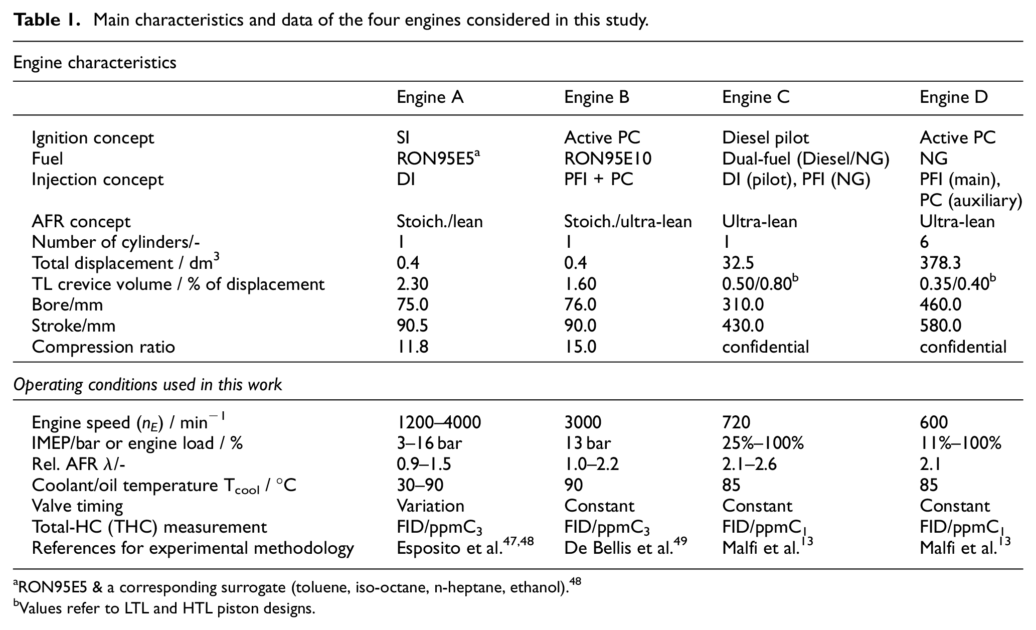
RON95E5 & a corresponding surrogate (toluene, iso-octane, n-heptane, ethanol).⁴⁸

Values refer to LTL and HTL piston designs.

The main development of the uHC model has been performed on the base of engine A because of the availability of a very extensive engine database, and 3D-CFD simulations.

All the considered measurements have been performed at stationary conditions, by setting a certain level of engine load in terms of indicated mean effective pressure (IMEP), engine speed (n_E), relative air-fuel ratio (λ), coolant and oil temperature (T_cool = T_oil). For engine A, the extensive emission database consists also of emission values at different sampling locations in the exhaust runner of the SCE. In total, for each selected operating point, 1000 consecutive cycles were recorded. Figure 1 reports a schematic of the Engine A SCE with the emission measuring positions relevant for the evaluation of uHC emissions in this study. Both values will be used for comparison against the simulated results.

Figure 1.

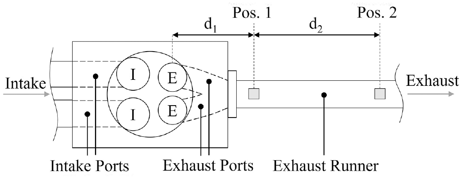
uHC measurement positions: the distances are approximately d₁ = 120 mm and d₂ = 400 mm.

Simulation model

3D-CFD RANS simulations

The 3D-CFD simulations considered in this study are the same as presented in Ref.,¹² performed according to the methodology explained in Ref.¹⁰ These 3D-CFD RANS investigations have been carried out with the software CONVERGE CFD v2.4 mainly to investigate the uHC formation mechanism from the piston top-land crevice. The data has been then post-processed to provide information to support and validate the modelling hypotheses and approach for the phenomenological uHC model. In particular, a geometrical post-processing of the 3D results from CFD has been coded in MATLAB and used to extract the trends of variables of interest in specific zones within the cylinder domain. A schematic and overview of the different zones evaluated in the post-processing is provided in Figure 2.

Figure 2.

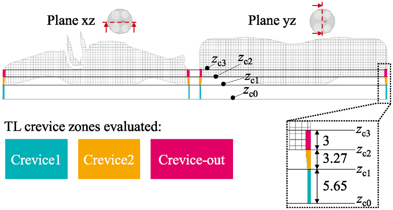
Illustration of the zone post-processing of the 3D-CFD results with details of the piston top-land crevice zones (dimensions are given in mm). Reworked from Ref.¹² with permission of SAE International.

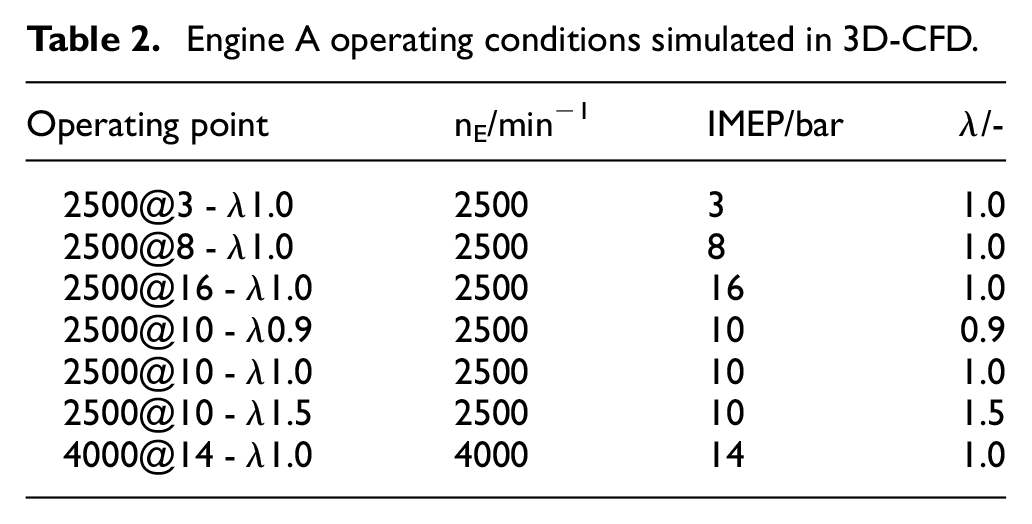
In Figure 2, z_c0 represents the base of the piston top-land crevice while z_c1 and z_c2 are the lowest and highest piston height respectively. The code for the zone post-processing uses as input the 3D-CFD cell-based results at a specific crank angle, the zones are identified based on cell coordinates, and the calculation of average quantities of interest is done in three separate zones around the TL crevices as depicted in Figure 2. All of them have ring-like forms. The zone ‘Crevice1’ consists of the lowest and narrowest zone of the TL crevice. The zone ‘Crevice2’ is directly above Crevice1 and reaches the piston shoulder. Since the piston is not flat, Crevice2 is a real crevice zone only for approximately 50% of the piston circumferential length. On the yz plane of Figure 2, it can be observed how Crevice2 really represents the gap between the piston and the liner while on xz plane, Crevice2 is a crevice outlet zone. The zone ‘Crevice-out’ is above Crevice2 and as wide as its outlet and it extends for 3 mm above the highest piston surface and allows the evaluation of the crevice outflow and oxidation thermodynamic state. The operating point simulated and considered for the development of the uHC phenomenological models are summarized in Table 2 and assume warm engine operation (T_cool = T_oil = 90°C).

Table 2.

Engine A operating conditions simulated in 3D-CFD.

Operating point	n_E/min⁻¹	IMEP/bar	λ/-
2500@3 - λ1.0	2500	3	1.0
2500@8 - λ1.0	2500	8	1.0
2500@16 - λ1.0	2500	16	1.0
2500@10 - λ0.9	2500	10	0.9
2500@10 - λ1.0	2500	10	1.0
2500@10 - λ1.5	2500	10	1.5
4000@14 - λ1.0	4000	14	1.0

Base 1D engine models

The GT-SUITE models used for the implementation of the uHC modelling include the geometry of the combustion systems between the low-pressure indication transducers, respectively in the intake and the exhaust runners as explained in Refs.^11,12 Measured instantaneous pressures and average temperatures are used as boundary conditions, as well as the rotational speed. The injected fuel is controlled by a PID controller to match the experimental air-to-fuel ratio. More details about the base model settings for engine A can be found in Refs.,^11,12 for engine B in Ref.,⁴⁹ and for engines C and D in Ref.¹³

The combustion model together with the uHC sub-models are both implemented in the GT-SUITE framework under the form of ‘user coding’. The combustion chamber is described by a two-zone approach, where the burned and unburned gases are subdivided into two zones at different temperatures and at the same pressure. To focus only on the predictivity of the uHC models, a combustion profile obtained from the analysis of the measurements through a three-pressure analysis (TPA) has been used to describe the combustion for the selected operating points. The uHC model is coupled to the combustion model by a burn rate manipulation process dependent on the release and post-oxidation uHC phenomena.¹³ The heat transfer calculation is managed using a modified Woschni correlation¹⁹ identified in GT-SUITE as WoschniGT with assumed wall temperatures for engine A as described in Ref.,¹¹ 3D-estimated temperatures for engine B and experimentally-derived temperatures for engines C and D.

Unburned hydrocarbon model

Among the main uHC mechanisms,¹² this work focuses on the piston top-land filling and emptying mechanism,^50–55 the wall flame quenching,^34,56 the adsorption and desorption of fuel from the oil layer^42,57 with the addition of a novel approach to estimate the fuel direct entry in the oil film for engine A.

In the following, both uHC formation and post-oxidation processes will be described for the four different formation sub-models considered in this study.

Top-land crevices – The developed model calculates the amount of mixture trapped in the TL crevice and its associated mass flow through the energy, mass and species balances. The energy balance for the gas trapped in the crevices can be written as:

\frac{dE}{dt} = - \frac{δ Q_{W}}{dt} + \frac{d m_{crev}}{dt} h_{flux}

(1)

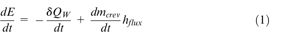
where E is the total energy in the crevice volume, δQ_W/dt is the wall heat transfer, dm_crev/dt is the mass flow rate from the cylinder, and h_flux represents the enthalpy of the volume where the flow flux originates. The mass and species balances are:

\frac{dm}{dt} = \frac{d m_{crev}}{dt}

(2)

\frac{d m_{k}}{dt} = \frac{d m_{crev}}{dt} Y_{crev, k}

(3)

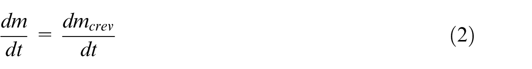
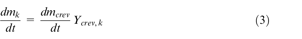
where Y_crev,k represents the mass fraction corresponding to the k-th species transferred between the cylinder and the crevice volume. Regarding the total internal energy, it can be calculated by multiplying the mass and the respective specific internal energy:

E = me

(4)

Therefore, if the mixture is considered as an ideal gas, the internal energy can be written as:

e = e_{0} + \int_{T_{0}}^{T} c_{v} dT

(5)

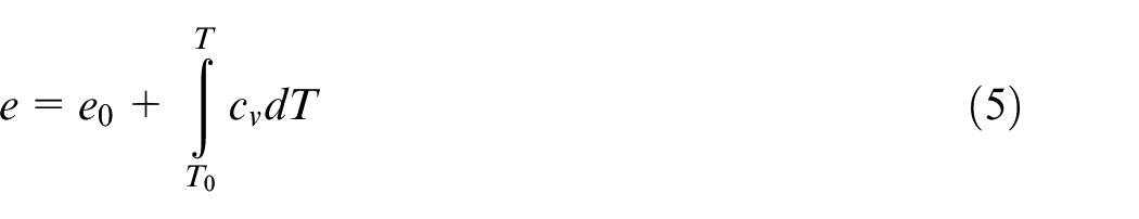
In which c_v represents the specific heat at a constant volume which generally relies on both the gas temperature, T, and its composition, x_k. Once assigned the crevice volume, V_tl, the gas density can be also evaluated. The thermodynamic state of the gas trapped in the crevices is univocally determined by the knowledge of instantaneous density and specific internal energy. Using the gas state equation, the pressure in the top land crevice can also be estimated.

The heat transfer coefficient, σ_crev, in the crevices is calculated through the definition of the Nusselt number, considering that the TL geometry predominantly extends in a specific direction:

σ_{crev} = \frac{N u_{crev} k_{crev}}{D_{crev}}

(6)

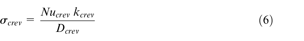
with k_crev representing the thermal conductivity of the trapped gas in the crevices, and D_crev indicating the crevice’s hydraulic diameter, defined as:

D_{crev} = \frac{4 A_{crev}}{P_{crev}}

(7)

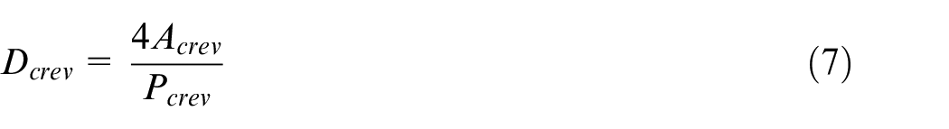
Here, A_crev represents the cross-section area of the crevices, taken perpendicular to its primary dimension, and P_crev is the cross-section wetted perimeter. The Nusselt number is calculated with the empirical correlation proposed in Ref.⁵⁸ The solution of mass and energy balances within crevices allows to estimate the instantaneous profiles of temperature and pressure, reported in Figure 3. The pressure trend is almost equal to that in the cylinder, while the temperature evolution strictly depends on the size and geometry of the crevices volume. The gas trapped in the TL crevice follows the unburned gas temperature evolution, with some delay and dimming related to the filling and emptying process and to the wall heat transfer.

Figure 3.

Exemplary model results for Engine A at operating condition 2500@3 - λ1 (cfr. Table 2): (a) average cylinder temperature with unburned and burned gas as well as crevices’ gas temperature and (b) cylinder pressure and pressure in the crevices.

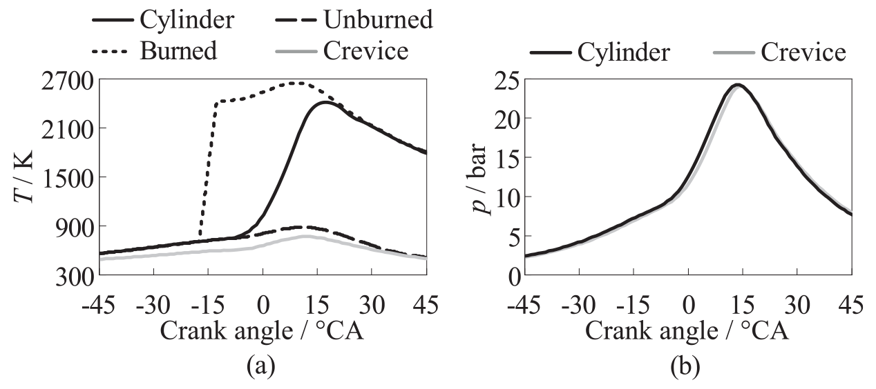
Usually, in literature, the crevice temperature is fixed at a constant value equal to that of the piston³⁰ or liner, or an average of the two temperatures. In a previous work,¹² the crevice temperature was calculated over the crank angle as a function of the temperatures of piston, liner and unburned gas with a specific formula that has been validated against 3D data. In this work, an alternative and more general approach is implemented in which the crevice temperature is calculated during the entire engine cycle from the energy balance equation. The calculated temperatures have been compared to the ones obtained through the 3D simulations to prove the approach reliability. In particular, both the Crevice1 and Crevice2 zones evaluated from CFD with geometric post-processing described depicted in Figure 2 are taken as reference. In Figure 4, the temperature comparisons have been depicted for all the available data. The crevice temperature from Esposito et al.¹² (black dotted line) reproduced a temperature profile similar to Crevice1 (cfr. Figure 2), which is the deeper and colder part of the TL crevice. The approach adopted in this study (black continuous line) overall shows similar temperature profiles to Ref.¹² with slightly higher levels in correspondence to the pressure peak, which can be considered more realistic considering also the temperature of the Crevice2 zone in CFD.

Figure 4.

Comparison among the 3D-CFD average temperatures in the zones Crevice1 (dashed grey line) and Crevice2 (dashed-dotted grey line), the simulated crevice temperature T_crev in this study (black continuous line) and calculated temperature T_crev from Esposito et al.¹² (dotted black line) for all the operating points simulated in 3D-CFD.

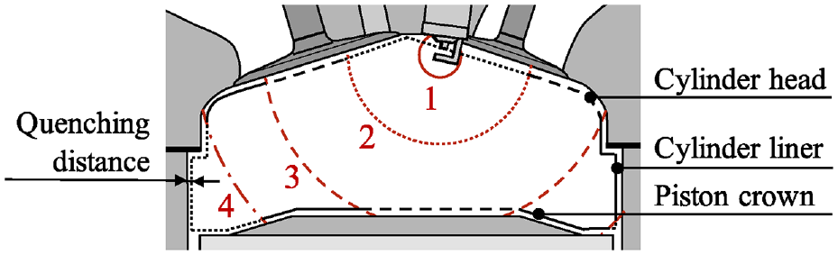
Flame wall quenching – To estimate the amount of the wall flame quenching, a simplified model for flame-wall interactions is employed. The quenched volume is evaluated by conceptualizing the combustion chamber as a cylindrical structure with a centrally located spark plug. The combustion chamber walls are then categorized into three distinct zones (Figure 5): cylinder head, cylinder liner and piston crown, each having its unique temperature. Beginning with the unburned gas volume, under the assumption of spherical flame propagation within a cylindrical combustion chamber, the real-time evaluation of the wall areas coming in contact with the advancing flame front is carried out.⁵⁹

Figure 5.

Combustion chamber areas schematization for wall flame quenching.

In Figure 5, representative flame configurations are depicted during four different instants of the flame progression. In the initial stage, the flame remains entirely detached from the cylinder walls (1); as it expands, a section of the flame front touches the cylinder head (2). Subsequently, the flame extends to reach the piston crown (3) and finally, the cylinder liner (4). The quenched volume variation can be estimated by multiplying the i-th combustion chamber wall areas (head, liner and piston) reached by the flame front in a time step by the quenching distances, δ_q,i = Pe_q,i· δ_fl, which is evaluated through the Péclet number (Pe_q,i) definition. Among all the terms cited above contributing to the evaluation of the quenching contribution, detailed in previous author work,¹³ a focus on the Péclet number estimation is posed. This term can be related to the normalized wall heat flux, φ_q, according to the correlation presented by Boust et al.^56,60:

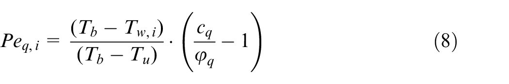
P e_{q, i} = \frac{(T_{b} - T_{w, i})}{(T_{b} - T_{u})} \cdot (\frac{c_{q}}{φ_{q}} - 1)

(8)

In the model presented, the normalized wall heat flux φ_q is held constant at 0.3, a value recommended in the situation of a laminar head-on quenching at ambient conditions.³⁴ The wall temperature T_w,i varies according to the specific region reached by the flame front, whether it is the cylinder head, liner, or piston. To correct the inaccuracies of the presented correlation, a tuning constant, c_q, is introduced in equation (8). By combining the quenching distances δ_q,i, and the area subject to the flame quenching, dA_q,i, with the gas density, it is possible to calculate the finite quenched mass in a time step. As a result, this mass, dm_q, is integrated over the engine cycle to compute the uHC contribution from wall quenching.

Oil layer – The modelling of the mechanism for uHC formation from the oil layer relies on the assumption of a dynamic equilibrium of desorption and absorption of the vaporized fuel into the oil layer. Within this model, the fuel concentration undergoes variations across different phases, shifting from the bulk gas to the oil film state. The mass flux occurring at the interface between these phases is determined by factors such as the Henry number, the mass transfer conductance of both gas and liquid phases, the mass concentration of vaporized fuel in the bulk gas phase, and the mass concentration of dissolved fuel within the oil film.²⁷ This mass flux is positive during the absorption of fuel into the oil film, and it reverses when desorption begins. The calculation of the fuel mass flow rate relies on the product between fuel flux into the oil and the surface area of the oil layer in contact with the gas mixture. This area is calculated in real-time accounting for the piston motion.

Fuel direct inclusion in the oil layer – In this work, an additional phenomenon is newly considered to contribute to the uHC emissions for the operating points at cold engine conditions. Indeed, the fuel injected into the combustion chamber that reaches the liner surface might directly be included in the oil layer,⁶¹ especially at low oil temperatures at which the fuel solubility in oil is increased. To mimic this additional source of uHC during the injection time, a fixed percentage of the injected fuel is assumed to be directly included within the oil layer and is directly added to the fuel mass in oil calculated by the mechanism described in the previous sub-section. During the expansion phase, this increased fuel quantity in the oil layer contributes to an increased fuel desorption from the oil layer thus, increasing the uHC production from this mechanism.

To quantify this additional uHC source, 3D-CFD calculations available for some representative operating points^10,12 for engine A are post-processed and the maximum percentage of fuel impinging the liner walls is evaluated and assumed as the amount of fuel that enters the oil film at cold engine conditions. Subsequently, based on 3D-CFD data, a correlation to estimate the injected fuel percentage forming the liquid film is developed depending on engine IMEP and λ values:

x_{fuel_inj} = 1.628 \cdot \ln (IMEP) + 2.271 \cdot λ - 3.544

(9)

Figure 6 reports the agreement between the fraction of injected fuel impinging the liner as evaluated in 3D-CFD and the estimation through equation (9). It can be observed that the amount is in the order of magnitude of 1%–4% and the developed correlation reproduces the 3D-CFD trend quite accurately for the different operating points.

Figure 6.

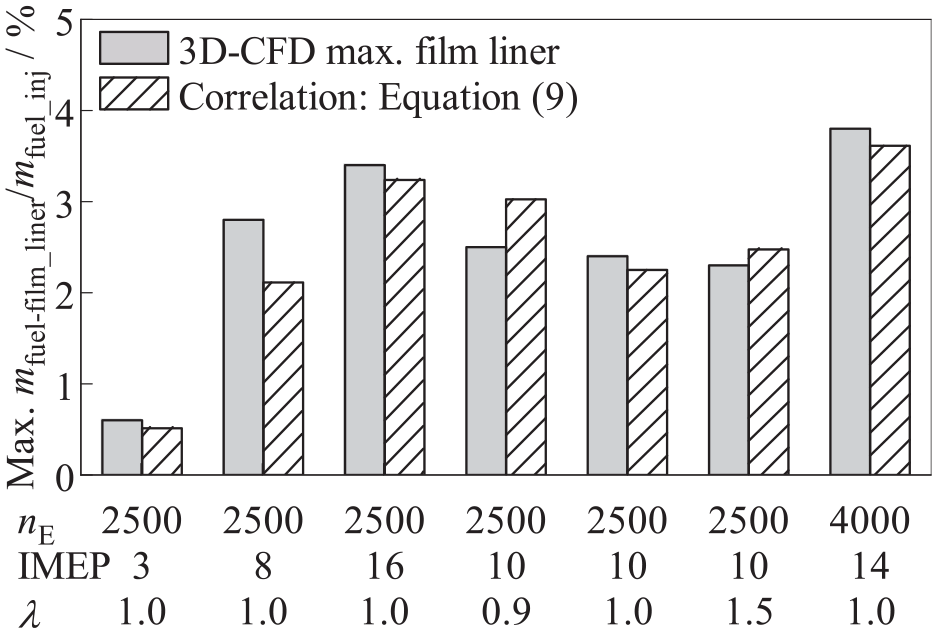
Estimation of fuel direct entry in the oil layer: comparison between 3D-CFD estimation and developed correlation from equation (9).

Boundary layer model – In order to reproduce appropriate conditions in terms of temperature and gas composition to evaluate the uHC post-oxidation rate, a boundary-layer based model has been developed. The presented approach aims to account for more realistic conditions at which the fuel oxidation process takes place, in contrast to conventional literature approaches assessed in the past.^62,63 Indeed, previous works usually consider an average temperature between wall and cylinder gas as reference oxidation temperature, and the concentrations considered for the oxidation of the species are average values for the entire cylinder. Previous work from the authors¹² estimated the temperature at which the uHC post-oxidation occurs as a function of wall and burned gas temperature variable over crank angle and showed a good reproduction of the temperature observed in the zone Crevice-out in 3D-CFD (see Figure 2), which represents the zone at which the oxidation of the uHC released from the piston TL crevice happens.

In this work, the boundary layer (bl) state is individually computed for various uHC-forming regions, namely crevices, wall quenching and oil layer. The calculations in those regions adopt a common mathematical approach. Regarding the uHC emissions from the TL crevice, the boundary layer represents a volume near the cylinder wall accumulating the mass exiting from crevices during the expansion phase. During this phase, the mass released from the TL crevice mixes with a part of the burned gas originating from the bulk burned gas region of the cylinder.

The temperature and volume of the boundary layer are evaluated on a crank angle basis by solving specific mass and energy balances expressed as:

\frac{d m_{bl}}{dt} = {\overset{\cdot}{m}}_{crev} + {\overset{\cdot}{m}}_{b}

(10)

\frac{d (m_{bl} \cdot e_{bl})}{dt} = {\overset{\cdot}{m}}_{crev} \cdot h_{crev} + {\overset{\cdot}{m}}_{b} \cdot h_{b} - p_{cyl} \frac{d V_{bl}}{dt}

(11)

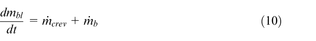
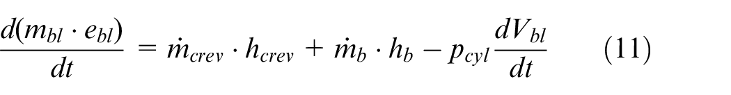
Here, m_bl represents the mass contained in the boundary layer, ṁ_crev the mass flow exiting from the top land crevice, ṁ_b is the entrained burned gas mass flow rate, e_bl is the specific internal energy of the boundary layer and V_bl is its volume, p_cyl represents the in-cylinder pressure, and h_crev, h_b and h_bl are the specific enthalpies of top land crevices, burned gas and boundary layer, respectively. ṁ_b characterizes the burned gas flux coming from the bulk region of the cylinder. This is defined to be proportional to the mass flux coming from the crevices through the tuning constant k_oxid (k_{oxid_crev} for the TL crevice):

{\overset{\cdot}{m}}_{b} = k_{oxid_crev} \cdot {\overset{\cdot}{m}}_{crev}

(12)

The energy balance for the boundary layer allows to estimate the temperature evolution for this cylinder region. In Figure 7, the calculated temperature trends for the crevices boundary layer are compared to the post-oxidation temperature modelled in Esposito et al.¹² and the temperature evaluated in the Crevice-out zone from 3D-CFD simulations (see Figure 2). In the proposed model, the post-oxidation process initialization corresponds to the rise of the boundary layer temperature. Hence, this happens after the top land crevice begins to release gases, after the cylinder peak pressure. This explains the absence of the BL temperature trend in the early stage of the expansion stroke, represented by the grey bands in Figure 7. The rest of the diagram represents the time at which the post-oxidation process occurs and hence the boundary layer region in the phenomenological model aims to reproduce a similar temperature. Indeed, it can be observed that the BL temperature quickly rises reaching a level that is in line with that in the Crevice-out zone from 3D-CFD simulations and similar to the post-oxidation temperature calculated in Ref.¹²

Figure 7.

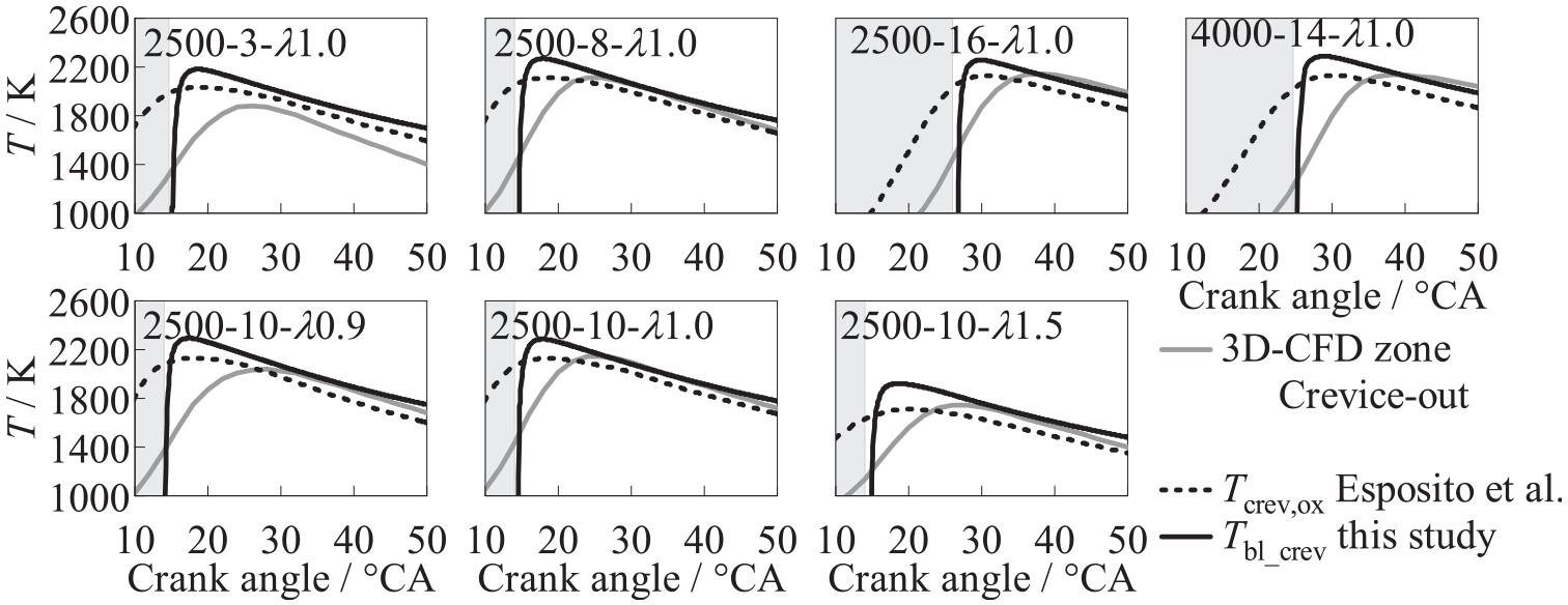
Comparison among the calculated boundary layer temperature for the TL crevice developed in this work, the average 3D-CFD temperature in the zone Crevice-out, and the previous approach to compute the TL crevice oxidation temperature from Esposito et al.¹² for all the investigated points with CFD. Grey bands highlight the instants before post-oxidation (and top-land crevice boundary layer model) activation.

As mentioned previously, the determination of the boundary layer state for the uHCs generated by wall flame quenching and absorption-desorption from oil follows a comparable approach to that used for the TL crevice. Concerning the wall flame quenching, one difference lies in the replacement of the production term ṁ_crev, attributed to the TL crevice, with the quenched mass rate, denoted as ṁ_quench, derived from the model detailed in the section above. Another variation consists in the quenching boundary layer which is assumed to not mix with the burned gas (ṁ_b = 0 in equations (10) and (11)), and the tuning constant k_oxid, in this case (k_{oxid_quench}), represents a weighting factor used to define the temperature of the gas in the boundary layer, whose level is between the temperatures of combustion chamber walls and burned gas, according to:

T_{bl_quench} = (1 - k_{oxid_quench}) T_{w} + k_{oxid_quench} T_{b}

(13)

The approach presented in equation (13) is different from the previous boundary layer model,¹³ but similar to that presented in Ref.¹² with the difference that the weighting factor there was between 0.2 and 0.3. The choice to have a separate boundary layer computation for the wall flame quenching arises from the necessity to account for a different release timing and thermodynamic state of the quenched mixture compared to those of the mixture released from the TL crevice. Indeed, the wall flame quenching happens in a phase of the expansion stroke with high and rising temperatures. Conversely, the TL crevice mixture is released after the peak pressure and encounters comparatively lower and decreasing temperatures. Adopting the same formulation for the boundary layer temperature would result in an unrealistic complete oxidation of the quenched mixture due to the high temperatures. Physically, to undergo post-oxidation, the quenched mixture needs to diffuse into the burned zone and this process has been proven to be a limiting factor for the post-oxidation of quenched layers.⁶⁴ To account for this slow diffusion, Esposito et al.¹² introduced a factor to strongly limit the post-oxidation of the wall flame quenching. In this work, k_{oxid_quench} accounts for this diffusion delay of the quenched layers into the hot burned gases. As far as the oxidation of uHC released from the oil layer is concerned, an approach similar to that adopted for the uHC oxidation from wall flame quenching is applied. This is controlled by the tuning constant k_{oxid_oil}, which acts as expressed by equation (13). A summary of the of the boundary layer calculations is schematized in Figure 8.

Figure 8.

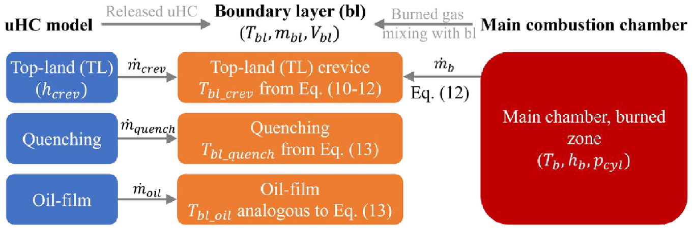
Sketch of the boundary layer areas and calculations considered in this work.

Post-oxidation kinetic modelling – As mentioned in Section 2, one-step kinetics is a common approach to describe uHCs post-oxidation. In previous work,¹³ a global kinetic reaction has been used for the evaluation of the oxidation rate of the released uHCs. This methodology is widely used because of the simplicity of application and the sensitivity of the main parameters involved in the oxidation process. However, this approach has some limitations. One of the main drawbacks is that the global kinetic reaction is a result of a fitting of different reaction processes, generally taken from experimental data or a detailed kinetic mechanism, in a quite wide set of engine-like conditions. This implies that the global reaction is not fitted for the actual condition present in the cylinder or the boundary layer but for an average engine condition. Another limit is the validity of the global reaction outside the conditions used for its evaluation.

As an advance of the existing models, a tabulated kinetic approach is here adopted for the oxidation process. This allows considering the exact conditions present in the boundary layer, both the thermodynamic state and the composition, improving the evaluation of the oxidation rate and allowing the application of the model within the thermochemical conditions used for the tabulation.

Similarly to previous works of the authors,⁶⁵ the chemistry tabulation is synthesized in a progress variable (and its derivative). This is defined as the formation enthalpy variation of the evolving mixture, computed with respect to a reference temperature of 298 K. The formation enthalpy (h_f) evolution is normalized by its variation between the final and beginning stages of the reaction process:

c = \frac{h_{f} (t) - h_{f} (t_{0})}{h_{f} (t_{end}) - h_{f} (t_{0})}

(14)

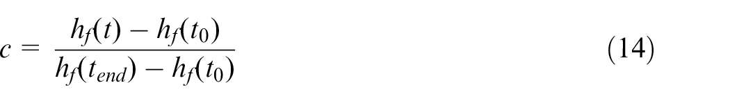
The progress variable time derivative, ċ_i, is tabulated in offline chemistry simulations in an adiabatic homogeneous reactor at 99 different and prefixed values of the progress variable, c_i, for various initial conditions of temperature, pressure, equivalence ratio and residual gas content. During engine simulations, the C-atom-based fuel equivalent oxidation fraction (r_ox), as already presented in previous work,¹² is calculated according to:

\int_{0}^{r_{ox}} \frac{dc}{\overset{\cdot}{c}} = Δ t

(15)

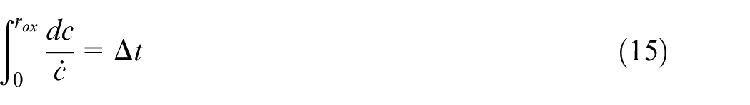
where Δt is the simulation time step and values of $\overset{\cdot}{c}$ are looked up from the above table at the current levels of temperature, pressure, equivalence ratio and residual content within the boundary layer. The integral in equation (15) is numerically solved by an algorithm where the upper bound of integration, r_ox, is iteratively changed until the equation is satisfied. The oxidation rate is finally used to calculate the mass of uHC that oxidizes during the time step:

m_{uHC, ox} = m_{uHC} \cdot r_{ox}

(16)

Results

Model calibration and sensitivity analysis

Before presenting the results of the uHC model, this section describes how the model can be tuned and what are the effects of its constants. Based on the description provided in the previous paragraphs, the constants to be selected for each engine are: c_q from equation (8) for the Péclet number estimation, and the three oxidation constants for TL crevice, wall flame quenching and oil layer, respectively (k_{oxid_crev}, k_{oxid_quench}, k_{oxid_oil}). To show the effect of the calibration constants on the model results, a sensitivity analysis is presented in Figure 9 for Engine A. In particular, the trend of the released uHCs (before post-oxidation) and post-oxidized concentration values are shown over crank angles for all the sub-models, (a) for the TL crevice, (b) for the wall flame quenching and (c) for the oil layer. Additionally, also the r_ox variable, which is evaluated in the boundary layer of each sub-model, is reported (right y-axis).

Figure 9.

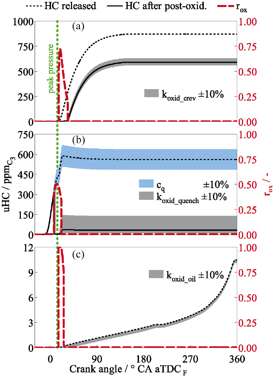
Instantaneous trends of uHC concentration before (released, dotted black line) and after the post-oxidation process (full black line) together with the r_ox variable that describes the post-oxidation (red dashed line). (a) Piston TL crevice, (b) wall flame quenching and (c) oil layer adsorption/desorption. Engine A: n_E = 1500 min⁻¹, IMEP = 3 bar, λ = 1.1.

Figure 9(a) shows that the TL crevice uHCs are released after the peak pressure when the combustion is almost complete, and oxidize intensely only for about 20° CA. This mechanism limits the production of uHC from this source until about 35° CA aTDC_F. Moreover, it is visible that the uHCs from flame wall quenching (Figure 9(b)) start to accumulate first, with a quite weak post-oxidation rate. The release of uHC from the oil layer (Figure 9(c)) also starts when the combustion ends, having an almost constant production rate and quite low levels.

A sensitivity analysis is superposed to all the representative trends shown in Figure 9. All four model constants are varied by ±10%. The variation of c_q is shown in the sub-plot (b) and highlighted through the light blue scatter band. For the k_oxid constants, the grey scatter bands highlight the sensitivity related to the ±10% variation. It can be observed that only the wall flame quenching model is quite sensitive to the variation of the model constants (namely c_q and k_{oxid_quench}) with strongly nonlinear behaviour due to the complex and high-temperature sensitivity of the wall quenching and its post-oxidation. The TL crevice sub-model shows approximately ±6% on the final uHC concentration with ±10% of k_{oxid_crev}, while the oil layer sub-model is almost insensitive to the variation of k_{oxid_oil}. This is due to the very late release of uHC when the temperature is too low for oxidation.

Regarding the tuning procedure, some steps are applied to identify the most appropriate set of constants, which are based on the following general observations. For the operating points at stoichiometric conditions and especially at high loads, the uHC production is expected to be dominated by the contribution of the crevices. The mass exchange between the top-land crevice and the cylinder is only determined by the instantaneous in-cylinder pressure and the geometric characteristics of the crevice volume, and no calibration parameters can control this phenomenon. Therefore, the final uHC contribution from crevices can be varied only by changing the intensity of the post-oxidation process through the constant k_{oxid_crev}, whose effect is depicted in Figure 9(a). This constant has been calibrated with a focus on the high-load points at stoichiometric conditions and kept constant for all other operating points. In the second step, the uHC production due to flame wall quenching is controlled by the c_q constant. This parameter allows increasing the quenching layer thickness at the wall and, as a consequence, it raises the quenching uHC emission especially at low loads and at diluted conditions. Then, the tuning on the post-oxidation of this uHC contribution through the constant k_{oxid_quench} as highlighted in Figure 9(b) allowed to improve the trends of uHCs, especially over λ. Finally, concerning the production of uHC from the oil layer, no actual tuning is applied, and also its post-oxidation is generally marginal whatever the value of k_{oxid_oil} as demonstrated in Figure 9(c).

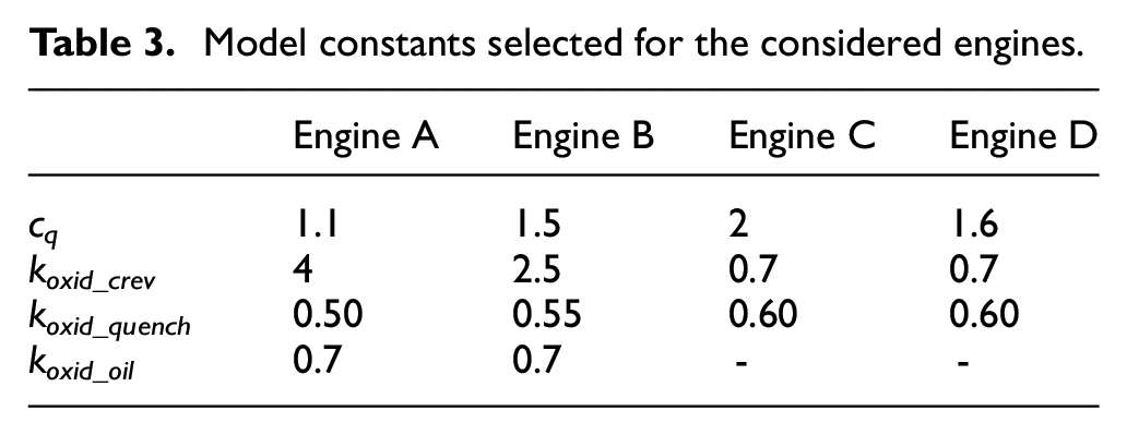
A summary of all the optimal values selected for the model constants for the considered engines is reported in Table 3. The model constants are kept fixed in all the operating conditions of each engine. It is worthwhile considering that the engines under study are very different in terms of dimensions, type of fuel, air/fuel proportions, mixture ignition mode and crevice size. Regarding the variability in c_q, this seems correlated with the mixture air-fuel ratio because engine A, which runs stoichiometric or close to stoichiometric, has a lower value than the other ultra-lean engines. Further differences among engines B, C and D can be related to the flame propagation in combination with the different geometries. Regarding k_{oxid_crev}, this looks strongly correlated with the TL crevice volume reported in Table 1. It is interesting to note that engines C and D, which have similar designs and the same main fuel (natural gas) have the same values for k_{oxid_crev} and k_{oxid_quench}, while the difference in c_q can be connected to the differences in the mixture ignition mode (pre-chamber fuelled with NG and diesel pilot, respectively) and consequent flame propagation. Both engines have no sub-model for oil layer adsorption/desorption because of the very high solubility of natural gas in oil, resulting in an early uHC release during expansion and an almost complete post-oxidation.

Table 3.

Model constants selected for the considered engines.

	Engine A	Engine B	Engine C	Engine D
c _q	1.1	1.5	2	1.6
k_{oxid_crev}	4	2.5	0.7	0.7
k_{oxid_quench}	0.50	0.55	0.60	0.60
k_{oxid_oil}	0.7	0.7	-	-

uHC prediction results

Figure 10 shows the comparison between predicted and measured cylinder-out uHC concentrations over the extensive database available for Engine A with variations in engine load, λ, valve timing and spark timing. The last load variation, λ variation and the spark timing variation are at cold engine conditions, where the coolant and oil temperature are maintained at 30°C instead of the standard level of 90°C, typical of warm engine operation. The spark timing variation at cold engine conditions represents the so-called ‘catalyst heating operation’ which has spark-timing retardation from optimal to very delayed combustion (until 10% coefficient of variation of IMEP is reached) at low load and low speed (n_E = 1200 min^−
1, IMEP = 3 bar, λ = 1.0). uHC measurement data (black lines) refers to two measurement positions along the exhaust line (see Figure 1). In particular, the overall model results (red continuous line) are shown together with the individual sub-models contributions (dashed blue line for TL crevice, dashed-dotted orange line for wall flame quenching, dashed-dotted green line for oil layer). For reference, the red dotted line shows the predicted values of the model from Esposito et al.¹² to show the improvements achieved in this study. It is quite visible how the prediction results follow the trends and the absolute levels of the measured uHC for all the operating conditions. As an example, the model predicts the reduction of uHC production at increasing load and speed (with stoichiometric air/fuel ratio), which is mainly due to the more intense post-oxidation process caused by higher in-cylinder temperatures. The model also detects the increase of uHC concentration in the case of lean air/fuel mixtures, which is related to the growth of wall flame quenching intensity (thicker quenching layer). The contribution of the oil layer is marginal in most cases but becomes essential to enhance the model predictivity at cold engine conditions. The simulation is also able to predict the trends and levels of uHC at catalyst heating operation, which is a very extreme operating condition. Compared to previous studies,^11,12 the actual model is able to capture better the trends over IMEP and λ, and above all, reaches very high accuracy at cold engine operation. This aspect is of major importance since the uHC prediction especially at a cold start is of central interest. It can be noted that for the EVC variations (lower row of Figure 10), the model shows a tendency to overestimate uHCs and it does not seem to perceive the effect of EVC retardation (increase of valve overlap). This might be due to 3D gas exchange and mixing effects with residual gases, which are not described in the current model. Globally, the presented model demonstrates to be accurate with an average deviation of 11.7% considering all the operating conditions of Figure 10.

Figure 10.

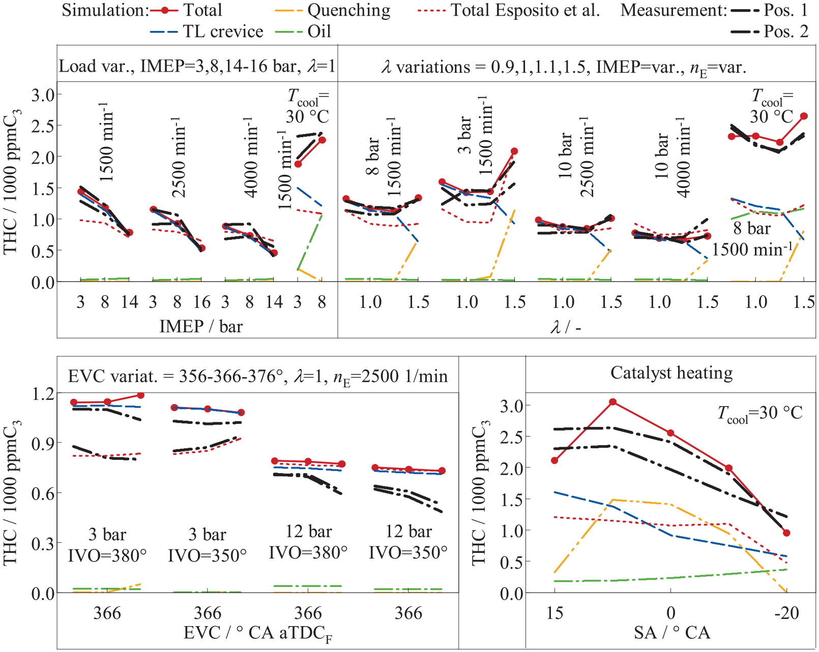
Experimental/simulation comparison of cylinder-out uHC concentration of Engine A. Upper row: load and λ variations; lower row: EVC and spark advance (SA) variation at catalyst heating conditions. Dotted red lines are the total predicted uHC from Esposito et al.¹² reported to highlight the improvement in the results achieved in this work.

Figure 11 presents the results of the uHC model for engines B, C and D. In this case, only one measurement dataset is used for comparison. As previously, single contributions of the uHC sub-models are reported in the figure. As far as engine B is concerned, a λ sweep at fixed engine speed and load is used for validation. Higher deviations are observed only at the first two richer points at λ=1 and 1.1, while the rest of the points show a very high accuracy of the predictions. On average, the deviation is 12.7% while it drops to 4.4% excluding the first two points. It is interesting to note how the trend of increasing λ is reproduced as a result of the quenching contribution.

Figure 11.

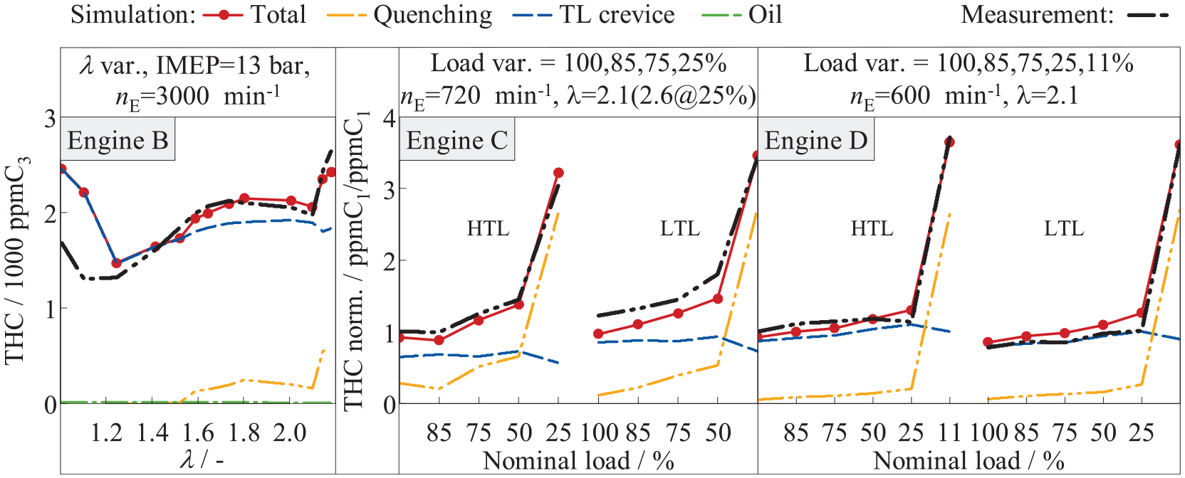
Experimental/simulation comparison of cylinder-out uHC concentration of Engine B (λ sweep), C and D (load sweep).

As far as engines C and D are concerned, the results consist of load variations at ultra-lean conditions for both ‘high top-land’ (HTL) and ‘low top-land’ (LTL) piston ring-pack configurations. The model predicts the increase of uHC production when the load decreases. This is mainly caused by an increase in the flame quenching layer thickness at the cylinder walls depending on the higher residual content, the mixture air-fuel ratio and on the lower cylinder pressure and temperature levels. On the other hand, the uHC production from the top-land slightly decreases with the load reduction, since a smaller amount of fuel is trapped in the crevice region when the in-cylinder peak pressure is lower. The simulation detects the effects of the ring pack dimension up to a certain extent since the piston design with the smallest top land height (LTL) leads to slightly reduced uHC emissions as shown in the experiments. The accuracy of the predictions is very high, and the average deviation observed is about 10% for both engines C and D and all the considered operating conditions.

As a final remark, it is worthwhile observing that the uHC model performs quite well for all studied engines, adopting similar calibration constants (see Table 3). This is a very important point in light of the substantial differences among the engines in terms of size, supplied fuel, rotational speed, air/fuel ratio and ignition system. This also allows to foresee the possibility of successfully applying the uHC model to further engines and fuels to evaluate their unburned fuel emissions in a pure predictive mode.

Assessment of model upgrades

In this final section, the advantages of the presented model improvements are highlighted. These can be summarized in three points:

1) Fuel inclusion in the oil layer at cold conditions.

2) Energy equation in the crevices replacing the isothermal hypothesis.

3) Post-oxidation computation by a tabulated approach instead of one-step chemistry.

The advantages of the first improvement can be inferred from the observation of Figure 10, where results for the Engine A conditions at 3 and 8 bar of IMEP and 1500 min⁻¹ are compared for two different coolant temperatures. This comparison highlights that uHC contributions from crevices and flame wall quenching have similar magnitude at cold and warm engine operation as to be expected based on thermodynamics (same IMEP means similar pressure and gas temperatures). However, as also well-known from literature,^14,66 the oil layer contribution becomes crucial at cold engine conditions because of the increased oil film thickness and increased fuel solubility in oil. Without the introduced enhancing mechanism of fuel entrainment within the oil layer, a poor uHC prediction would have been found under cold conditions, resulting in uHC levels similar to those estimated under warm operations as visible also in the results from Esposito et al.¹²

Figure 12 shows the impact of the model improvements 2) and 3) for three load variations and four λ variations for the Engine A. Concerning the introduction of the energy equation to estimate the temperature into the crevices, the advantages can be observed in Figure 12 comparing the actual final results of this work (red lines) with results obtained by fixing the temperature of the gas into the crevices equal to that of the piston (dashed teal lines). The comparison is performed by superimposing the crevice boundary layer temperatures since these temperatures have been verified against CFD results as shown in Figure 7. The average deviation on the selected points varies from 7.2% to 29.7% demonstrating the improvement associated to the crevice temperature calculation.

Figure 12.

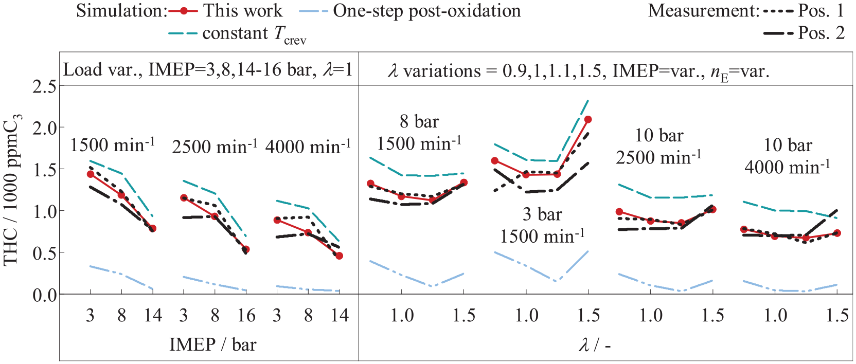
Comparison of uHC results from this work (red lines) against results in isothermal hypothesis for crevice gas (dashed teal lines) and results obtained with one-step chemistry for uHC post-oxidation (dot-dashed light blue lines).

Finally, the model enhancement deriving from the new post-oxidation approach can be observed again in Figure 12 by comparing the actual final results of this work (red lines) with results obtained through the application of the well-assessed one-step chemistry approach^{26,27,30,31,43–45} (dot-dashed light blue lines). Once again, these results have been obtained maintaining the same crevice boundary layer temperature. In this case, the average deviation of the predicted uHC for the considered points increases from 7.2% up to 83.9% demonstrating the potential need for an arbitrary recalibration of the one-step approach and the advantage of the here proposed post-oxidation method based solely on tabulated chemistry.

Concerning the same type of comparisons for engines B, C and D, regarding model improvement 2), the average deviations of the predicted uHC increase from 12.7% up to 15.0%, from 10.7% up to 11.7% and from 9.5% up to 29.7%. Regarding model improvement 3), the average deviations for engines B, C and D, increase from 12.7% up to 63.2%, from 10.7% up to 26.0% and from 9.5% up to 20.5%. Also, for these engines, the results have been obtained maintaining the same crevice boundary layer temperature to evaluate model improvements 2) and 3). The obtained results confirm increased predictivity of the here proposed model.

Summary and conclusions

This work has presented further developments to a model for the prediction of unburned hydrocarbons emitted by internal combustion engines. Starting from the authors’ previous work,^11–13 model approaches have been refined in order to increase the level of physical description of the adopted phenomenological models. New modelling aspects like the direct fuel inclusion in the oil film have been considered. The model is developed with the help of 3D-CFD simulations and validated against four different engines including two small-bore single-cylinder engines fuelled with gasoline, and two large-bore naval engines fuelled with natural gas. The model capabilities to predict uHC are very high at a very wide range of operating conditions including cold start, very different engine designs, fuels and ignition sources. In total, 83 different engine operating conditions from the four engines have been considered for the validation and the average deviation is 11.4%.

The model proves to correctly describe the major effects contributing to uHC and incomplete fuel combustion in a physical manner. Therefore, the model is suitable for the future virtual development of new combustion concepts. With the right update of model constants, the model could be extended to predict unburned fuel emissions from engines fuelled with alternative potentially non-fossil fuels like methanol, hydrogen, or ammonia. Future work will focus on the extension and validation of the models in combination with those fuels.

Footnotes

Appendix

Acknowledgements

The authors are thankful to Convergent Science Inc. for providing licences for the CONVERGE software.

Declaration of conflicting interests

The author(s) declared no potential conflicts of interest with respect to the research, authorship, and/or publication of this article.

Funding

The author(s) disclosed receipt of the following financial support for the research, authorship, and/or publication of this article: This work was partially funded by ‘Deutsche Forschungsgemeinschaft’ (DFG – German Research Foundation) – GRK 1856. The 3D-CFD simulations were performed with computing resources granted by RWTH Aachen University under project ‘rwth0239’.

ORCID iDs

Enrica Malfi

Stefania Esposito

Massimiliano De Felice

References

Reitz

Ogawa

Payri

, et al. IJER editorial: the future of the internal combustion engine. Int J Engine Res 2020; 21: 3–10.

Onorati

Payri

Vaglieco

, et al. The role of hydrogen for future internal combustion engines. Int J Engine Res 2022; 23: 529–540.

Senecal

Leach

Diversity in transportation: Why a mix of propulsion technologies is the way forward for the future fleet. Results Eng 2019; 4: 100060.

Leach

Kalghatgi

Stone

Miles

The scope for improving the efficiency and environmental impact of internal combustion engines. Transp Eng 2020; 1: 100005.

Kalghatgi

Is it really the end of internal combustion engines and petroleum in transport?

Appl Energy 2018; 225: 965–974.

Khan

MZA

Khan

Ravi

Turner

Aziz

Potential of clean liquid fuels in decarbonizing transportation – an overlooked net- zero pathway?

Renew Sustain Energ Rev 2023; 183: 113483.

Kalghatgi

Is it the end of combustion and engine combustion research? Should it be?

Transp Eng 2022; 10: 100142.

Morcinkowski

Adomeit

Mally

Esposito

Walter

Yadla

. Emissionsvorhersage in der Entwicklung ottomotorischer EU7-Antriebe. In: Liebl

(eds) Experten-Forum Powertrain: Ladungswechsel und Emissionierung 2019. Proceedings, (2020). Wiesbaden: Springer Vieweg.

Maurer

Yadla

Balazs

, et al. Designing zero impact emission vehicle concepts. In: Liebl

(ed.) Experten-Forum Powertrain: Ladungswechsel und Emissionierung 2020. Berlin, Heidelberg: Springer, 2021, pp.75–116.

10.

Esposito

Mally

Cai

Pitsch

Pischinger

Validation of a RANS 3D-CFD gaseous emission model with space-, species-, and cycle-resolved measurements from an SI DI engine. Energies 2020; 13: 4287.

11.

Esposito

Diekhoff

Pischinger

Prediction of gaseous pollutant emissions from a spark-ignition direct-injection engine with gas-exchange simulation. Int J Engine Res 2021; 22: 3533–3547.

12.

Esposito

Diekhoff

Pitsch

, et al. Development of phenomenological models for engine-out hydrocarbon emissions from an SI DI engine within a 0D two-zone combustion chamber description. SAE technical paper 2021-24-0008, 2021.

13.

Malfi

De Bellis

Bozza

, et al. A phenomenological model for the description of unburned hydrocarbons emission in ultra-lean engines. Int J Engine Res 2022; 23: 995–1011.

14.

Hochgreb

Chapter 6 - Combustion-Related Emissions in SI Engines, In: Eran

(ed), Handbook of Air Pollution From Internal Combustion Engines. Academic Press, 1998; pp. 118–170.

15.

Cheng

Hamrin

Heywood

, et al. An overview of hydrocarbon emissions mechanisms in spark-ignition engines. SAE technical paper 932708, 1993. DOI: 10.4271/932708.

16.

Alkidas

AC.

Combustion-chamber crevices. Prog Energy Combust Sci 1999; 25: 253–273.

17.

Alkidas

AC.

The effects of head gasket geometry on engine-out HC emissions from S.I. engines. SAE technical paper 1999-01-3580, 1999. DOI: 10.4271/1999-01-3580.

18.

Amano

Okamoto

Unburned hydrocarbons emission source from engines. SAE technical paper 2001-01-3528, 2001. DOI: 10.4271/2001-01-3528.

19.

Heywood

JB.

Internal combustion engine fundamentals. New York: McGraw-Hill, 1988, p.930.

20.

Alkidas

Drews

Miller

. Effects of piston crevice geometry on the steady-state engine-out hydrocarbons emissions of a S.I. engine. SAE technical paper 952537, 1995. DOI: 10.4271/952537.

21.

Adamczyk

Kaiser

Lavoie

GA.

A combustion bomb study of the hydrocarbon emissions from engine crevices. Combust Sci Technol 1983; 33: 261–277.

22.

Wentworth

JT.

Piston and ring variables affect exhaust hydrocarbon emissions. SAE technical paper 680109, 1968. DOI: 10.4271/680109.

23.

Wentworth

JT.

The piston crevice volume effect on exhaust hydrocarbon emission. Combust Sci Technol 1971; 4: 97–100.

24.

Adamczyk

AA.

Hydrocarbon emissions from an annular crevice: effects of spark/insert position, equivalence ratio and pressure. Combust Sci Technol 1989; 64: 263–276.

25.

Haag

Heuer

Krämer

, et al. Reduction of hydrocarbon emissions from SI-engines by use of carbon pistons. SAE technical paper 952538, 1995. DOI: 10.4271/952538.

26.

D’Errico

Ferrari

Onorati

, et al. Modeling the pollutant emissions from a S.I. engine. Warrendale, PA: SAE International, 2002. DOI: 10.4271/2002-01-0006.

27.

Dorsch

Neumann

Hasse

Application of a phenomenological model for the engine-out emissions of unburned hydrocarbons in driving cycles. J Energy Resour Technol 2016; 138: 022201.

28.

Min

Cheng

WK.

Oxidation of the piston crevice hydrocarbon during the expansion process in a spark ignition engine. Combust Sci Technol 1995; 106: 307–326.

29.

Trinker

Cheng

Davis

GC.

A feedgas HC emission model for SI engines including partial burn effects. SAE technical paper 932705, 1993. DOI: 10.4271/932705.

30.

Sodré

Yates

DA.

An improved model for spark ignition engine exhaust hydrocarbons. SAE technical paper 971011, 1997. DOI: 10.4271/971011.

31.

Schramm

Sorenson

SC.

A model for hydrocarbon emissions from SI engines. SAE technical paper 902169, 1990. DOI: 10.4271/902169.

32.

Frølund

Schramm

Simulation of HC-emissions from SI-engines - a parametric study. SAE technical paper 972893, 1997. DOI: 10.4271/972893.

33.

Oliveira

Hochgreb

Effect of operating conditions and fuel type on crevice HC emissions. SAE technical paper 1999-01-3578, 1999. DOI: 10.4271/1999-01-3578.

34.

Suckart

Linse

Schutting

Eichlseder

Experimental and simulative investigation of flame–wall interactions and quenching in spark-ignition engines. Automot Engine Technol 2017; 2: 25–38.

35.

Lorusso

Kaiser

Lavoie

GA.

In-cylinder measurements of wall layer hydrocarbons in a spark ignited engine. Combust Sci Technol 1983; 33: 75–112.

36.

Schramm

Sorenson

SC.

Solubility of gasoline components in different lubricants for combustion engines determined by gas—liquid partition chromatography. J Chromatogr A 1991; 538: 241–248.

37.

Huang

Pan

, et al. An investigation on simulation models and reduction methods of unburned hydrocarbon emissions in Spark Ignition Engines. Combust Sci Technol 1996; 115: 105–123.

38.

Min

Effects of the oil and liquid fuel film on hydrocarbon emissions in spark ignition engines. Proc IMechE, Part D: J Automobile Engineering 2002; 216: 759–771.

39.

Yildirim

Gul

Ozatay

Karamangil

. Simulation of Hydrocarbon Emissions from an SI Engine. SAE Technical Paper 2006-01-1196, 2006, https://doi.org/10.4271/2006-01-1196.

40.

de Albuquerque

PCC

de Andrade Ávila

Barros Zárante

Sodré

JR.

Lubricating oil influence on exhaust hydrocarbon emissions from a gasoline fueled engine. Tribol Int 2011; 44: 1796–1799.

41.

Ihsan Karamangil

Sürmen

Yenice

. Mathematical modeling of hydrocarbon emissions from oil film for different fuels. Fuel 2014; 115: 818–825.

42.

Dent

Lakshminarayanan

PA.

A model for absorption and desorption of fuel vapour by cylinder lubricating oil films and its contribution to hydrocarbon emissions. SAE technical paper 830652, 1983. DOI: 10.4271/830652.

43.

Sodré

JR.

Further improvements on a HC emissions model. SAE technical paper 1999-01-0222, 1999. DOI: 10.4271/1999-01-0222.

44.

Tinaut

Melgar

Horrillo

AJ.

Utilization of a quasi-dimensional model for predicting pollutant emissions in SI engines. SAE technical paper 1999-01-0223, 1999. DOI: 10.4271/1999-01-0223.

45.

Da Silva

LLC

Nigro

FEB

. Modeling of hydrocarbons formation and emission in gas engines. SAE technical paper 2000-01-2038, 2000. DOI: 10.4271/2000-01-2038.

46.

Eng

Leppard

Najt

, et al. The effect of fuel composition on hydrocarbon emissions from a spark ignition engine: iso-octane/toluene and n-octane/toluene fuel mixtures. Warrendale, PA: SAE International, 1998. DOI: 10.4271/982557.

47.

Esposito

Mauermann

Lehrheuer

, et al. Effect of engine operating parameters on space- and species-resolved measurements of engine-out emissions from a single-cylinder spark ignition engine. SAE technical paper 2019-01-0745, 2019. DOI: 10.4271/2019-01-0745.

48.

Esposito

Cai

Günther

Pitsch

Pischinger

Experimental comparison of combustion and emission characteristics between a market gasoline and its surrogate. Combust Flame 2020; 214: 306–322.

49.

De Bellis

Malfi

Bozza

, et al. Experimental and 0D Numerical Investigation of ultra-lean combustion concept to improve the efficiency of SI engine. SAE Int J Adv Curr Pr Mobil 2021; 3: 1993–2008.

50.

Bignion

Spicher

. Investigation of the influence of top land crevice geometry on hydrocarbon emissions from SI engines. SAE technical paper 982560, 1998.

51.

Christensen

Johansson

Hultqvist

The effect of piston topland geometry on emissions of unburned hydrocarbons from a homogeneous charge compression ignition (HCCI) engine. SAE technical paper series. Warrendale, PA: SAE International, 2001.

52.

Namazian

Heywood

JB.

Flow in the piston-cylinder-ring crevices of a spark-ignition engine: effect on hydrocarbon emissions, efficiency and power. SAE technical paper 820088, 1982. DOI: 10.4271/820088.

53.

Min

Cheng

Heywood

JB.

The effects of crevices on the engine-out hydrocarbon emissions in SI engines. SAE technical paper 940306, 1994.

54.

Angstrom

Königsson

Kuyper

, et al. The influence of crevices on hydrocarbon emissions from a diesel-methane dual fuel engine. SAE Int J Engines 2013; 6: 751–765.

55.

Smith

Cheng

Heywood

. Crevice volume effect on spark ignition engine efficiency. SAE technical paper 2014-01-2602, 2014.

56.

Boust

Sotton

Labuda

Bellenoue

A thermal formulation for single-wall quenching of transient laminar flames. Combust Flame 2007; 149: 286–294.

57.

Min

Cheng

WK.

Oil layer as source of hydrocarbon emissions in SI engines. J Eng Gas Turbine Power 1998; 120: 669–677.

58.

De Bellis

Malfi

Bozza

, et al. A thermodynamic model of a rapid compression expansion machine applied for the estimation of the flame speed of air/hydrogen mixtures. Fuel 2023; 341: 127657.

59.

Grill

Billinger

Bargende

Quasi-dimensional modeling of spark ignition engine combustion with variable valve train. SAE technical paper 2006-01-1107, 2006.

60.

Boust

Bernard

Sotton

, et al. A model of flame quenching in non-isothermal initial conditions. In: 4th European combustion meeting, Vienne, Austria, 14 April 2009.

61.

Alzahrani

Fatouraie

Sick

Analytical model for liquid film evaporation on fuel injector tip for the mitigation of injector tip wetting and the resulting particulate emissions in gasoline direct-injection engines. Int J Engine Res 2022; 23: 49–63.

62.

Jensen

Schramm

The role of post flame oxidation on the UHC emission for combustion of natural gas and hydrogen containing fuels. Warrendale, PA: SAE International, 2003.

63.

Kuppa

Nguyen

Goldmann

, et al. Numerical modelling of unburned hydrocarbon emissions in gas engines with varied fuels. Fuel 2019; 254: 115532.

64.

K-C

Hochgreb

Chemical kinetic simulation of hydrocarbon oxidation through the exhaust port of a spark ignition engine. Combust Flame 1996; 107: 383–400.

65.

De Bellis

Malfi

Lanotte

, et al. A tabulated chemistry multi-zone combustion model of HCCI engines supplied with pure fuel and fuel blends. Energies 2022; 16: 265.

66.

Froelund

Schramm

Tian

Wong

Hochgreb

Analysis of the Piston Ring/liner oil film development during warm-up for an SI-engine. J Eng Gas Turbine Power 2001; 123: 109–116.

Phenomenological model for unburned hydrocarbon emissions from spark-ignition,pre-chamber,and dual-fuel internal combustion engines

Abstract

Keywords

Introduction

Sources and modelling of uHC

Methodology

Experimental data

Simulation model

3D-CFD RANS simulations

Base 1D engine models

Unburned hydrocarbon model

Results

Model calibration and sensitivity analysis

uHC prediction results

Assessment of model upgrades

Summary and conclusions

Footnotes

Appendix

Acknowledgements

Declaration of conflicting interests

Funding

ORCID iDs

References