
Abstract
The cold start process for a gasoline direct injection (GDI) engine was studied through multidimensional simulations using a Fractal Engine Simulation (FES) model integrated into CONVERGE CFD. The simulations were focused on the very first firing cycle in the cold start process, as most of the hydrocarbon emissions derive from this cycle. The dramatically changing engine speed and low wall temperatures in the cylinder present challenges for simulation. It turned out that the FES model was able to predict the in-cylinder pressure traces for all four cylinders for the first firing cycle, and gave good agreement with the experimental measurements under these extremely transient conditions. More comprehensive analysis demonstrated the causes for the different behavior of the combustion in different cylinders: more injected fuel and a higher induced tumble ratio in cylinder 3, the first to fire, led to a higher average equivalence ratio and better fuel distribution, which resulted in the highest peak pressure; the worse fuel distribution from the lower tumble ratio, together with the lower normalized turbulence, caused weaker combustion in cylinder 4; the peak pressures were similar and on the low side for cylinders 2 and 1, mainly determined by the low average equivalence ratio. An improved strategy with multiple injections was proposed, with the first two in the intake stroke and two later injections in the compression stroke rather than one injection during each stroke. Although the total injected fuel was the same as the baseline strategy, more fuel evaporated due to the enhanced fuel evaporation from both droplets and wall films, resulting in a higher average equivalence ratio in the cylinder. The peak cylinder pressure and IMEP rose by 33.3% and 8.4%, respectively, using the 4-injection strategy compared to the baseline 2-injection strategy, and the 4-injection strategy was verified by the experiments, as well.
Keywords
Introduction
Gasoline direct injection (GDI) engines work by injecting the fuel directly into the combustion chamber, where it can mix with air, as opposed to port fuel injection (PFI) engines, where the fuel is injected into the intake port. The GDI engine has been studied extensively and developed rapidly since it first appeared on the market, where it is now dominant for its improved fuel economy, higher engine efficiency, and reduced engine emissions. Based on the 2021 EPA automotive trends report, 1 the market share for light-duty vehicles equipped with GDI has been increasing and reached a new high of 57% in model year 2020, compared to 2.3% in model year 2008. However, the cold start emissions for a GDI engine, especially for the first several firing cycles, remain a key problem due to the more stringent emissions standards for model year 2025.
In a cold start process for a GDI engine, the fuel rail pressure (FRP) is much lower than the normal working pressure, leading to poor atomization. The unevaporated injected fuel forms liquid films when it impinges on the wall, and the evaporation from the wall wetting is a very slow process due to the low vapor pressure and the cold walls. The unevaporated portion will escape the combustion process and may eventually contribute to engine-out emissions. Moreover, the catalysts in the after-treatment system cannot be fully operational because the temperature is below the light-off temperature of around 250°C. 2
Different experimental3–6 and simulation7–11 studies have been used to focus on what happens during the cold start process and what may be done to reduce the emissions. Efforts are needed in the experiments to eliminate the wall wetting and maintain a cold wall to mimic a cold-start environment, which introduces extra work and difficulties. Computational fluid dynamics, on the other hand, can provide detailed information about the complicated physics happening in the engine, extend understanding, and suggest the directions for improvements. As a result, more and more researchers provide both experiment and simulation results for a complementary purpose.
Malaguti et al. 7 investigated the fuel film formation and mixture preparation for low-temperature cranking operation of a GDI engine, with the help of the three-dimensional simulation platform, Star-CD. Their research provided understanding of the origins of spark-plug fuel deposits, and suggested some improvements in injection management. Xu et al. 8 studied the effects of engine speed and injection timing for a GDI engine based on a Ford in-house CFD code. They also stated that a wider piston bowl design could produce the most robust mixture cloud for ignition. Morita et al. 10 et al. used Star-CD to study how a stratified mixture was formed during fast idle conditions, and proposed a “variable exhaust valve-timing system” to reduce the hydrocarbon emissions. Ravindran et al. 11 proposed a modified version of the G-Equation combustion model for capturing the flame propagation under cold-start conditions in a direct injection spark ignition (DISI) engine.
All these simulations were carried out using different constant engine speeds. However, as indicated by the cycle-to-cycle experimental measurements in a prior study by our research team, 12 most of the hydrocarbon (HC) emissions originate in the very first firing cycle of the cold start, and then decrease gradually. Therefore, the very first firing cycle should be given special attention. For this, a constant engine speed cannot be used in the simulation, since the engine speed increases sharply during the firing events in the very first firing cycle, and different combustion intensities were observed for different cylinders due to the effects of the transient engine speed. As pointed out in another study 13 of ours, the transient conditions, including transient engine speed, fuel vapor pressure, and fuel rail pressure, are critical to consider during the engine cold start simulations which will otherwise yield different results.
The remainder of this paper is structured as follows. The engine configuration and the experimental details are shown first. The settings in the multidimensional simulations are covered, including different models used in CONVERGE CFD and an overview about the Fractal Engine Simulation model. Next, the simulated results are presented for all four cylinders in the very first firing cycle under cold start conditions, and the conditions that result in different combustion intensities are demonstrated and analyzed in detail. Finally, a new strategy is put forth and the potential capability is shown to enhance the evaporation process, and consequently, the following burning process. Validations and comparisons with experiments are provided as well.
Engine configuration
In this study, a Ford 2017-model-year 4-cylinder 2.0-liter turbocharged gasoline direct injection (GDI) engine was used. The bore and stroke were 87.5 and 83.1 mm, respectively, and the compression ratio was 10:1. The geometry of the engine is shown in Figure 1, with two intake valves and two exhaust valves per cylinder. The six-hole fuel injector could provide up to 200 bar of fuel pressure. The engine employed a baseline dual-injection strategy during the cold start process, with an early injection happening during the intake stroke to provide a homogeneous background fuel distribution, and a late injection during the compression stroke to provide a rich fuel cloud near the spark plug region for ignition. The firing order of the four cylinders was 3-4-2-1 in the engine, and all four cylinders had the same engine timings shown in Figure 2 for the first firing cycle of cold start.
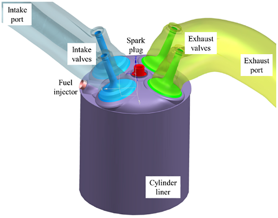
Engine geometry in this research.
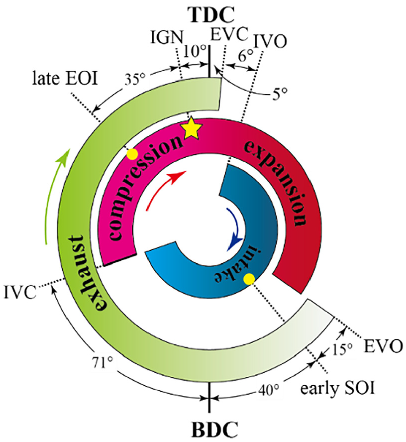
Engine timings in the cold start process: TDC: top dead center; BDC: bottom dead center; IGN: time of ignition; SOI: start of injection; EOI: end of injection; EVO: exhaust valve opening; EVC: exhaust valve closing; IVO: intake valve opening; IVC: intake valve closing.
Experiment setup
The engine in this cold start research was set in an environmental chamber with a controlled ambient temperature of 22°C ± 1°C. A water brake dynamometer was connected to the engine’s flywheel to generate a simulated idle load. A National Instruments cRIO system was used to replace the engine control unit (ECU) so that different parameters could be easily tuned in the engine. The in-cylinder pressure for all four cylinders were tracked using a 4-channel oscilloscope connected to the pressure transducer charge amplifiers. The high-resolution transient engine speed was captured and calculated based on the pulse signals of a rotational incremental encoder, which was installed on the flywheel. Figure 3 depicts a schematic diagram of the experimental setup, and more information can be found in previous papers12,14 from our team.
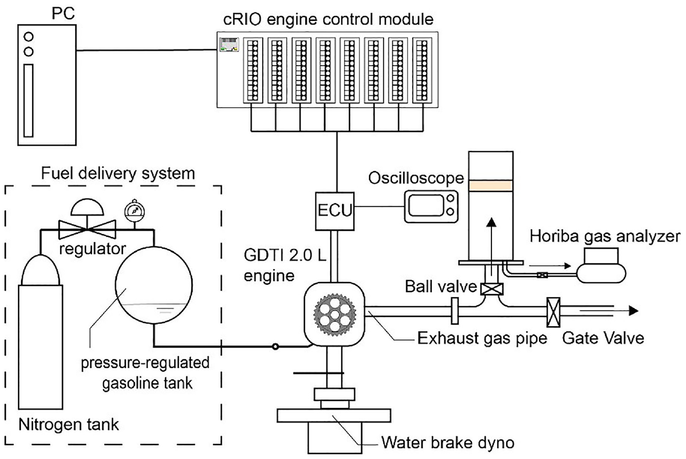
Schematic diagram of the cold start experiment. 14
The instantaneous engine speed from the experiments for the very first firing cycle was used in the cold start simulations. Figure 4 presents 10 curves of engine speed, coming from 10 different cold start experiments on different days. The trends of these curves were very similar, though there were slight differences. The compression TDC for cylinder 3, 4, 2, and 1 corresponded to 0, 180, 360, and 540 CAD, respectively, according to the firing order 3-4-2-1. Thus, the engine speed would increase sharply right after these TDCs, and then gradually decreased as the combustion progressed and exhaust valves opened. The process repeated for each of the four firing events in each cylinder, and the engine speed finally increased from around 300 RPM to about 1200 RPM. The transient engine speed led to different pressure traces in different cylinders and was critical to consider in the cold start simulations, which will be shown later. One of these curves was arbitrarily chosen to be used in the simulations as there would be no significant differences if other curves had been used. For more consistent comparisons among the four events, the fuel rail pressure (FRP) was kept constant at 80 bar for all cylinders in the experiments through external fuel rail pressurization which was independent from the production rail pressure control system.
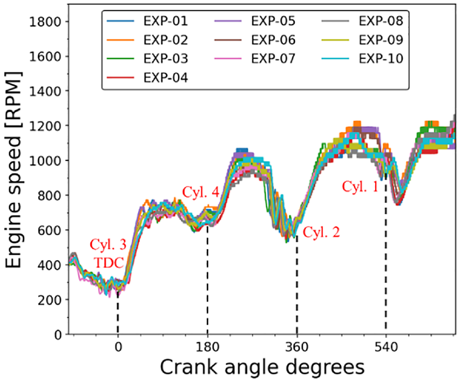
Transient engine speed curves in the very first firing cycle.
CFD model
CONVERGE CFD™ (CONVERGE for short), a commercial three-dimensional CFD package widely used in engine simulations, was used to perform all simulations in this study. Autonomous meshing in CONVERGE makes it easy to accommodate complex moving geometries, saving a significant amount of time for users. It will repeat the mesh generation process when the piston or the valves move, and produce a finer/coarser mesh as necessary for the simulations. We applied fixed embedding in the mesh as well, for those regions where a finer resolution was critical to the accuracy of the solution, including but not limited to the regions near the injections when simulating the sprays, the valve surfaces during their movements, and the spark plug gaps during the ignition period. Furthermore, another technique named adaptive mesh refinement (AMR) was implemented to locally refine the grid for the regions where the temperature or the velocity changed dramatically, without unnecessarily slowing the calculation with a globally refined grid.
Two full cycles were used for simulating the very first firing cycle, with the first one simulating the cranking cycle used for engine synchronization in the experiments, and the second one simulating the combustion process. Often in engine simulations, the first simulation cycle is used to set the flow conditions for the following cycle of interest and establish the residual gas quantity. This was not the purpose in our case since we were simulating the first cycle to fire. A constant pressure was used at the inlet and outlet surfaces throughout the simulation. The manifold air pressure (MAP) was measured in the experiments, and it fluctuated within only 3% of the ambient pressure before IVC of the last cylinder to fire. Thus, the same average value was taken for all four cylinders in the simulation. We did not include any acoustic/manifold tuning effects in the simulation, and no effects of interaction between different cylinders were considered for the intake and exhaust sides, which were assumed negligible in the current study. As the interest was the very first firing cycle after the engine sat overnight, room temperature was assigned to all the wall surfaces as the boundary conditions.
Different models were used in the simulation to resolve the complicated physics in the engine. Turbulence was modeled using the standard k-ε model of the Reynold-Averaged Navier-Stokes (RANS) method. During the injection process, the droplet breakup was predicted using the modified Kelvin-Helmholtz and Rayleigh-Taylor (KH-RT) model. 15 No Time Counter 16 (NTC) and Post and Abraham Collision Outcomes 17 methods were employed for droplet collisions. The O’Rourke model 18 was used to simulate the effects of turbulent flow on the droplets. The droplet-wall interactions were described using the wall film model.
One goal of the paper is to analyze the average flow features in the very first firing cycle resulting from the cold-start conditions. The RANS model is primarily focused on capturing the ensemble-averaged behavior of the turbulent flows, and in our case represents ensemble-averaged mean flow characteristics that would be representative of a typical individual cold start cycle; of course, cycle-to-cycle variations are always present in any actual engine cycle. Although measurements in different experiments are provided below, the simulation results are always compared to the results averaged in the very first firing cycle.
The Fractal Engine Simulation (FES) model19,20 was used to simulate the combustion phenomenon. It uses the fractal geometry 21 in mathematics to account for the flame surface wrinkling, and calculates the turbulent flame speed from the local fractal dimension and the laminar flame speed, shown as equation (1).
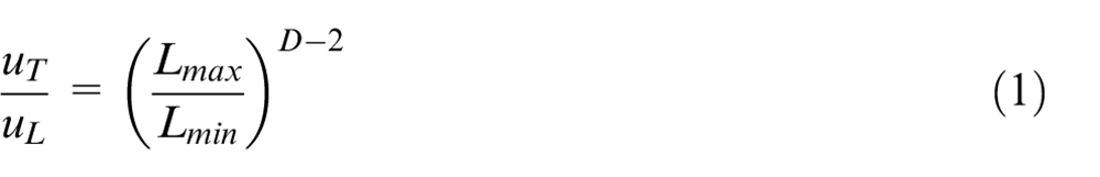
where

where
Iso-octane was used as the fuel for the reaction kinetics, and considering the importance of vapor pressure in cold start simulations, the vapor pressure was changed to that of gasoline having a Reid vapor pressure (RVP) of 7, with true vapor pressure (TVP) calculated from Moshfeghian’s correlations. 27 Unlike Figure 4, where TDCs for different cylinders are presented at different crank angles in a sequential manner, the TDCs of the four cylinders are shifted to 720 CAD in the results shown below for better and easier comparison.
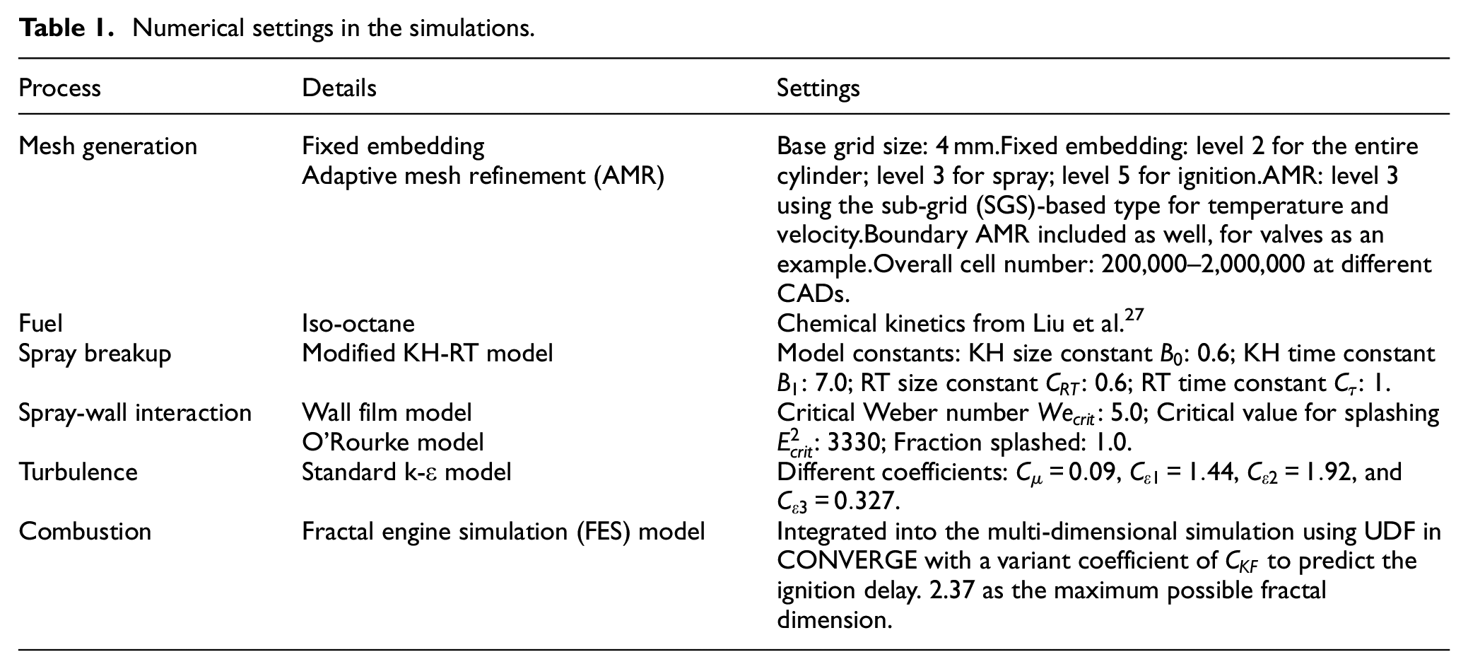
Some detailed settings in the simulation are provided in Table 1.
Numerical settings in the simulations.
Simulation results
Results in four cylinders
Pressure traces from five experiments for all four cylinders and the FES results are shown in Figure 5. For each cylinder, four experimental curves stayed quite close to each other, while the combustion in one curve was weak compared to the others. This was caused by cyclic variations in the bulk flow, making turbulence levels and fuel distribution different in different cycles, and thus making the ignition or combustion unstable. However, the predictions using the FES model are always compared to those robust combustion cycles in the experiments. The magnitude and location of peak pressure, averaged from the four robust combustion cases, with the experimental 95% confidence intervals, are presented as the dots and error bars in Figure 5. The simulated results for cylinders 3 & 2 matched well with the experiments, while the simulated peak pressures were a bit low for cylinders 4 & 1, due to the possible extra evaporated fuel in the experiments introduced from the back flow of evaporated fuel into the intake manifold during the compression stroke from cylinders 3 & 2 and subsequently inducted into cylinders 4 and 1, respectively. 26 The resulting indicated mean effective pressure (IMEP) was slightly lower for the last cylinder to fire, cylinder 1 (3.4% below the lower 95% confidence limit), but stayed within the confidence intervals for the other three cylinders.
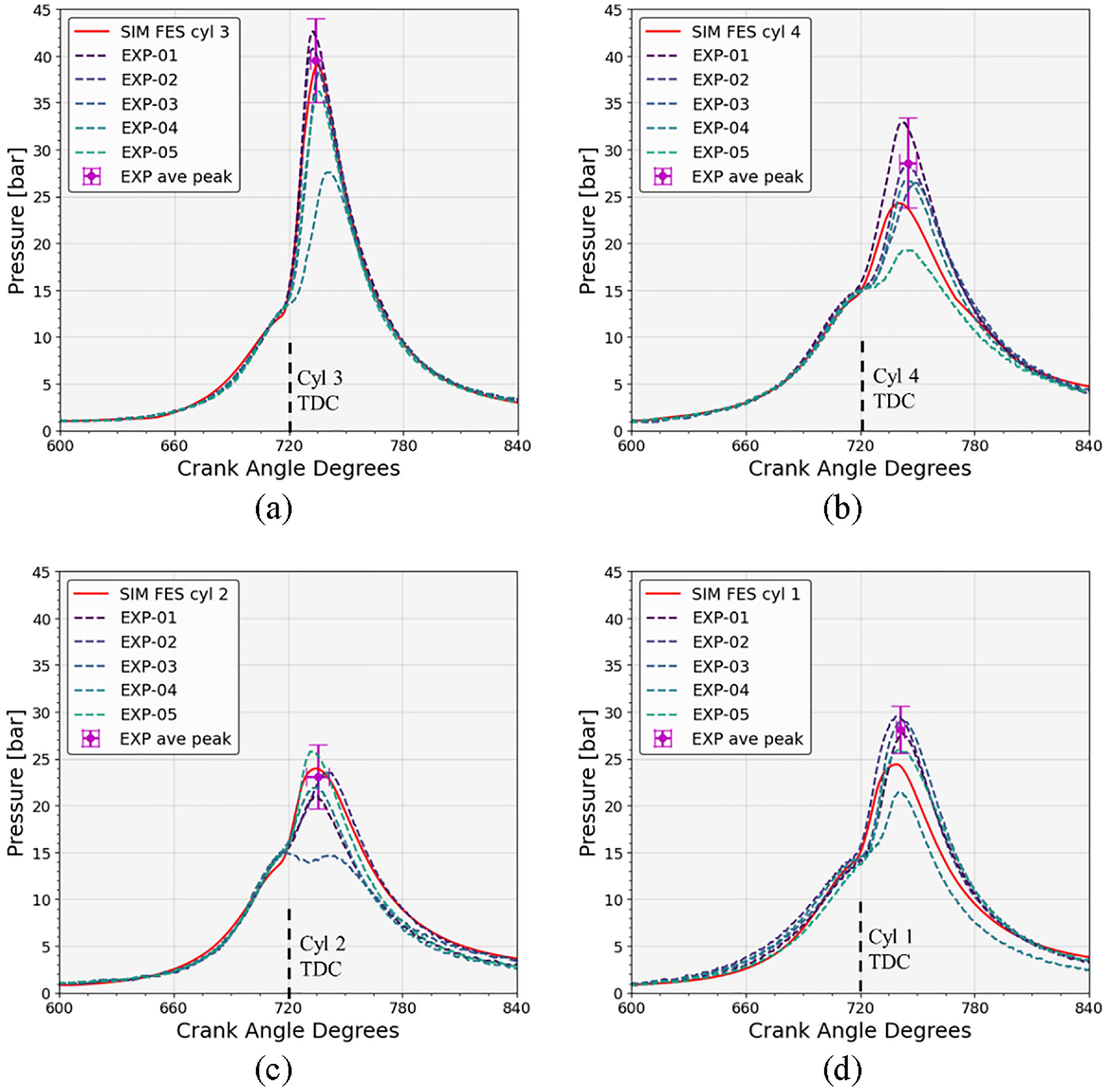
In-cylinder pressure traces for different cylinders: red solid curves for simulation results, and all dashed curves for five different experiments: (a)–(d) for cylinder 3, 4, 2, 1, respectively, based on the firing order; pink dots for experimental average peak pressures, with error bars calculated from the four robust experiments.
In general, the FES predictions were comparable to the experimental measurements: all the initial combustion events matched well with the experiments; the peak pressures in cylinders 3 and 2 fell among the four robust combustion curves, whereas they were a little lower for cylinders 4 and 1, but the differences were not huge; the phasing of the peak pressure was comparable as well; the trends for the combustion in different cylinders appeared the same, strongest in cylinder 3, while relatively weak and close for the other three cylinders.
More detailed validations about the FES model are presented in the paper, 26 including apparent heat release rate (AHRR), integrated heat release (IHR), and additional different operating parameters (a sweep of ignition timings). The slight deviations in the compression stroke between the simulation and experiment pressure traces in Figure 5 are caused by a small amount of twisting of the shaft-encoder coupling when the extremely transient engine speed was measured during the very first firing cycle, which is discussed extensively in the paper. 26
Detailed analysis of different cylinders
One interesting fact inferred from the peak pressure shown in Figure 5 is that the combustion was much stronger for cylinder 3 (the first to fire), while it was weak and quite similar for the other three cylinders. This was mainly determined by the average vapor-phase equivalence ratios and fuel distributions in the different cylinders, which is the main focus of this section.
Fuel tracking at the time of ignition for each cylinder is shown in Figure 6, where the bars with different colors indicate the mass percent of the fuel in different locations. The shaded bars (both blue and red portions) represent the total evaporated percent at the time of ignition. The percentage was similar for cylinders 3 & 4, and higher than cylinders 2 & 1, where it was very close as well. Although the same FRP and injection timing were used, different cylinders presented different characteristics for fuel evaporation, mainly due to the different transient engine speeds. Different intensities of turbulence and tumble/swirl flow were expected due to the different engine speed records (see Figure 4), affecting the mixing and evaporation process for different cylinders. These complex effects can be visualized as close but different curves in the 0–0.033 s range of Figure 7(a) for the early injection and 0–0.0032 s of the zoomed-in figure in Figure 7(a) for the late injection, where the mass percent for the evaporated fuel in the actual time space is shown. A more significant factor influenced by the engine speed variation was the residence time of the fuel sprays and films in the cylinder: a lower speed resulted in a longer residence time for the fuel in cylinders 3 & 4, leading to gradually increasing, but finally higher total percent of evaporation (Figure 7(a)), relative to cylinders 2 & 1. Note that the intake stroke for cylinder 3 is not shown in Figure 4, but the engine speed was about 350 RPM as it was just cranking; the engine speed at SOI of early injection for cylinder 4 was about 300 RPM, which was before the engine sped up.
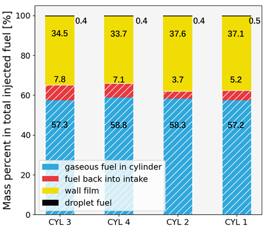
A fuel tracking at the time of ignition for different cylinders: the bars represent the mass percent in total injected fuel; blue bars for gaseous fuel in cylinder, red for fuel back into the intake ports, yellow for the wall wetting, and black on top for the droplet fuel in cylinder; the shaded bars indicate the total evaporated mass.
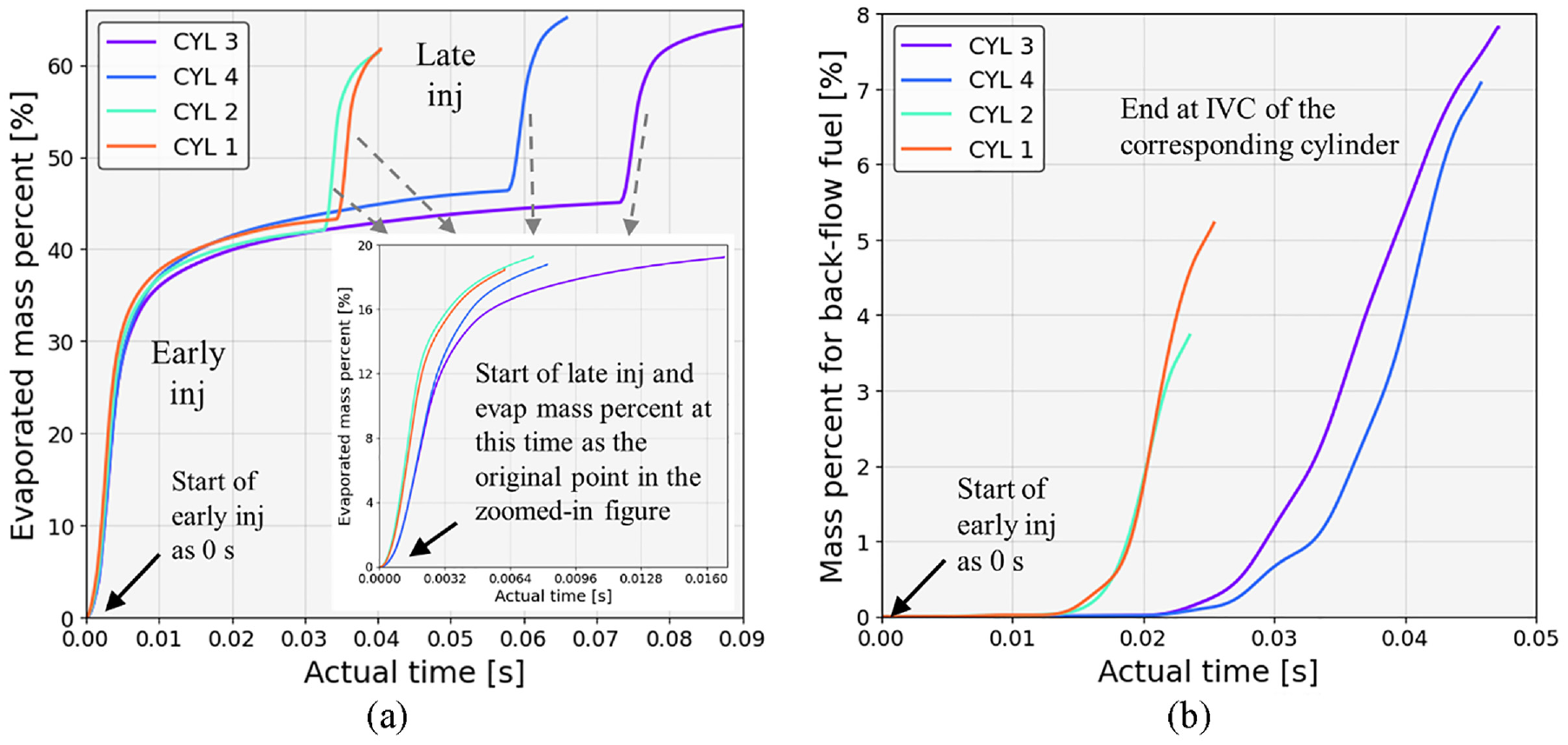
Evaporated fuel mass percent of total injected fuel as a function of actual time: evaporated fuel from SOI to 700 CAD in (a); fuel back into the intake ports from SOI (early) to IVC of each cylinder in (b). Although the same timings in crank angle are used for different cylinders, the durations in the actual time space are different due to different transient engine speeds.
Although more fuel evaporated in the first two cylinders to fire, the fraction (blue bars in Figure 6) which remained in the cylinder was about the same for each; the difference came from the fuel that flowed back into the intake ports during compression (shown as the red bars in Figure 6) as the momentum of intake air was not strong enough at the low engine speeds between BDC and late IVC. In general, the fraction of the back-flow fuel increased with time as the piston rose between intake BDC and IVC, and the back-flow was delayed and extended at lower engine speeds, as displayed in Figure 7(b), showing the relation between the back-flow fuel percent and the actual time starting from the SOI of early injection. It is worth noting that although the gaseous fuel fractions in different cylinders were almost the same, the average equivalence ratios for cylinders 3 & 4 were greater than cylinders 2 & 1, shown as the blue curve in Figure 8. There are two reasons for this: (1) 9% more fuel was injected in the first two cylinders, a representative typical fuel injection strategy for cold start; (2) the total mass of fresh air inducted into the cylinder was almost the same at BDC, but back-flow with different durations (in actual time) caused a greater retention of air in cylinders 2 & 1 (100%:101.3%:103.8%:102.8% for relative mass of fresh air in each cylinder at IVC, following the firing order). Different amounts of air in each cylinder also had an impact on the in-cylinder pressure traces between IVC and TDC, which was not huge, but can be observed in Figure 5.
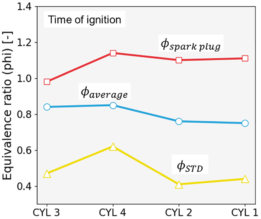
Equivalence ratios at the time of ignition in different cylinders: blue curve for the average equivalence ratio, red for equivalence ratio around the spark plug, and yellow for the standard deviations of the equivalence ratio.
Presented in Figure 8, the equivalence ratio around the spark plug is about 1.1 for cylinders 4, 2, & 1, which is very close to the optimal equivalence ratio, where the laminar flame speed is the highest, whereas it is less than 1 for cylinder 3. This indicates that the initial combustion was the slowest in cylinder 3, though the later combustion was the strongest, as explained below, compared to the other cylinders.
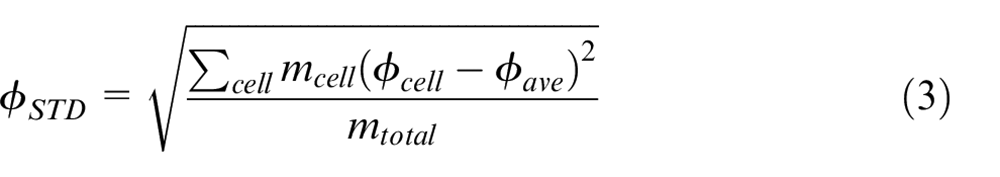
The fuel spatial distribution at the time of ignition is another key parameter for GDI engines, which is indicated by the standard deviation (
The highest
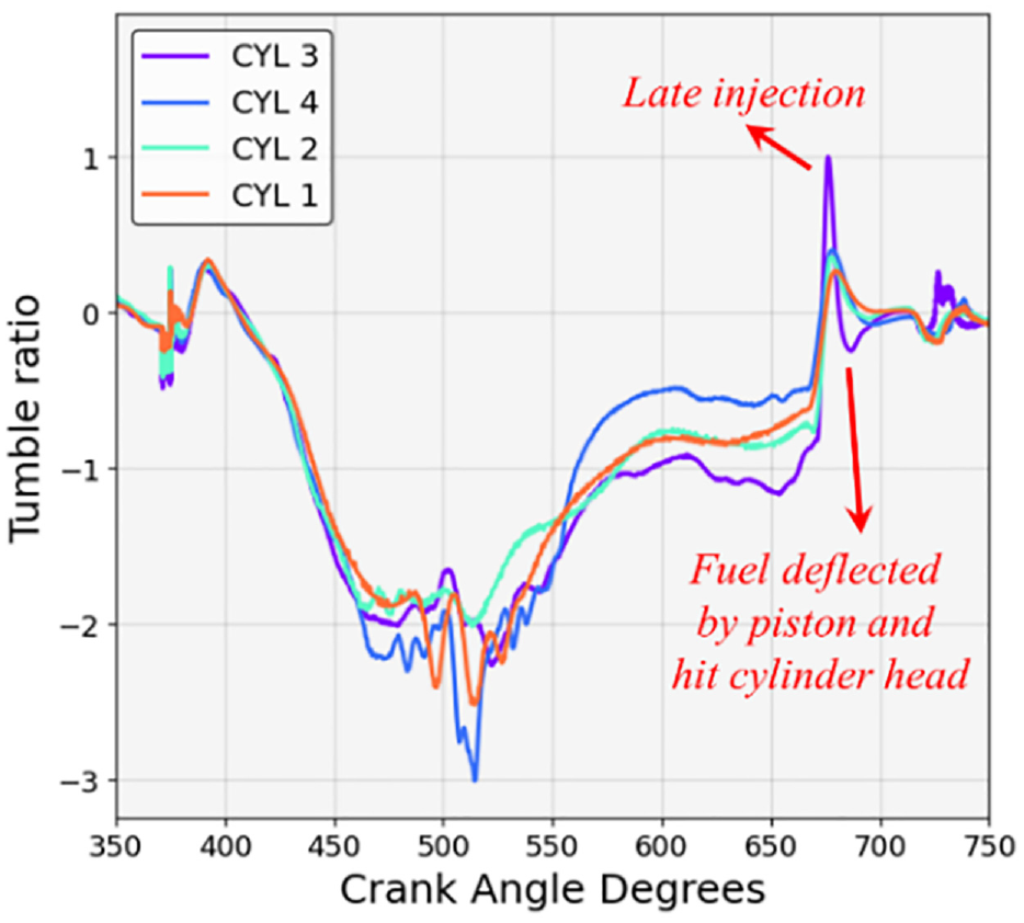
Tumble ratios in the different cylinders with crank angles.
The transient engine speed during the cold start process introduced more difficulties in predicting the fluid motion in the cylinder, but basically stronger fluid motion was maintained for a higher average engine speed, which was more resistant to the same induced momentum by the injections (same FRP). Thus, the induced tumble ratio was obvious for cylinder 3 (cranking engine speed, basically), and very weak for the other three cylinders (engine speed was higher than 600 RPM), where the second peak was hardly seen.
The fuel concentrations for late injection are clearly visualized in Figure 10, where the equivalence ratio distributions for different cylinders at different crank angles are presented. The fuel was injected into the cylinder and hit the piston bowl at 675 CAD, and was deflected to the cylinder head at 680 CAD. Then the fuel would move and diffuse in the cylinder such that the mixture became more and more uniform. As seen for cylinder 3, at the lowest engine speed (most mixing time) and highest induced tumble ratio, the fuel spread to the other regions, becoming more uniform. Despite the lower tumble ratio in cylinders 2 and 1, the homogeneity of the air-fuel mixture at 700 CAD was even better than, or at least similar to cylinder 3, as less fuel was injected in cylinders 2 & 1 than cylinder 3. The same results are indicated quantitatively by
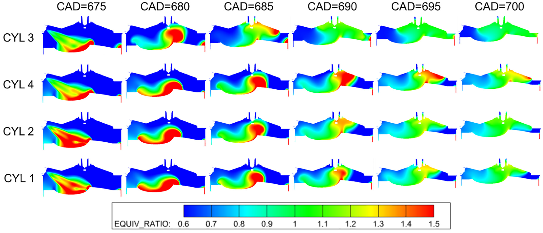
Equivalence ratio distributions in different cylinders at different crank angles; ignition occurs at 10 CA° BTDC, TDC is 720 CA°.
Another parameter which can affect the intensity of combustion is the turbulence level in the cylinder. As demonstrated in one
13
of our previous papers about cold start, the mass fraction burned (
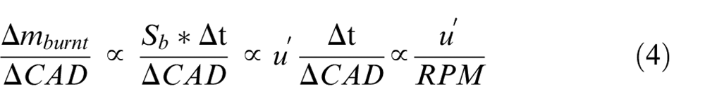
Thus, the RPM-normalized turbulence intensity should be compared among the four cylinders with their different engine speeds. The engine speeds (
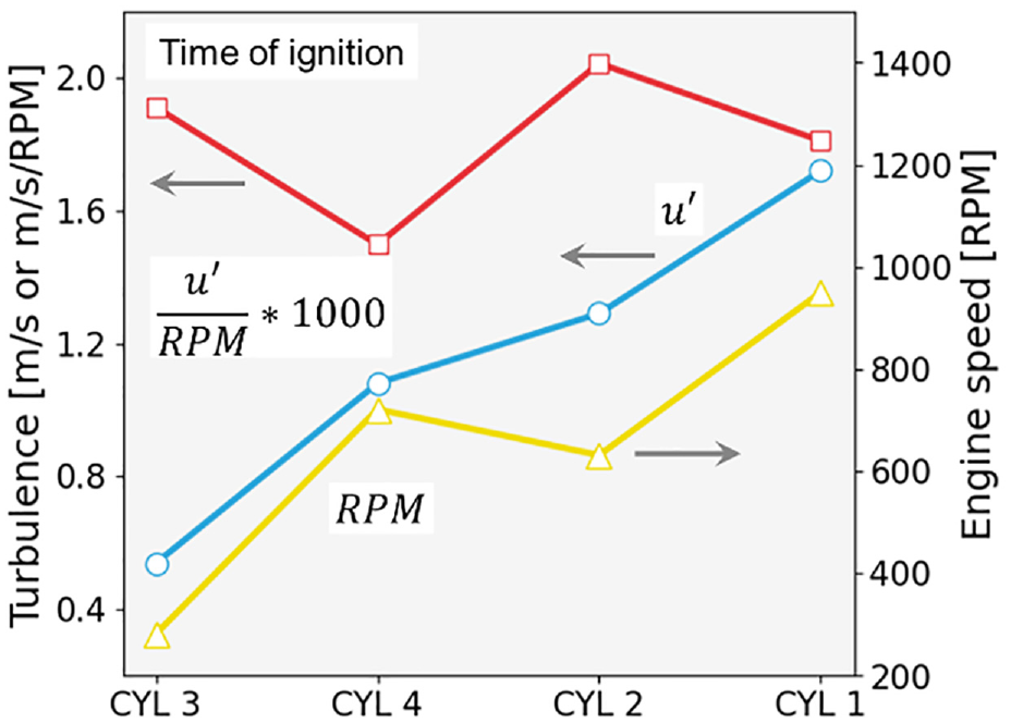
Turbulence levels and engine speed of different cylinders at the time of ignition.
The combustion behavior in different cylinders can be explained when Figures 8 and 11 are considered together. More injected fuel led to a higher average equivalence ratio for cylinders 3 and 4, and the better in-cylinder fuel distribution for cylinder 3 resulted in stronger combustion with a peak pressure achieved around 40 bar. The mixture inhomogeneity, together with the low normalized turbulence, inhibited the overall combustion rate for cylinder 4, and the peak pressure reached only 25 bar, which was very close to that of cylinders 2 and 1, where similar parameter values (
Improved strategy
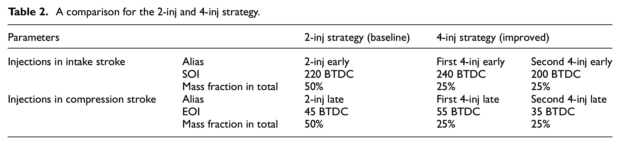
Using the FES’s capability of simulating non-uniform turbulent combustion shown above, an improved strategy (4-injection strategy) with multiple injections was studied. In the new strategy, both the early and late injections (as described in Figure 2) were further subdivided into two injections each, with an injected mass split ratio of 50%−50%, while the total injected mass in the intake and compression stroke was kept the same as the baseline strategy. The baseline (Figure 2) and the improved strategy will be denoted by the 2-inj and 4-inj strategy below, respectively, and the detailed parameters describing these two strategies are presented in Table 2.
A comparison for the 2-inj and 4-inj strategy.
The simulations were carried out for cylinder 3, which was the first one to fire in the very first firing cycle. To present the combustion intensities using both strategies, the pressure traces from both experiments and simulations are shown in Figure 12, where all five experimental curves are for the 4-inj strategy, and the experimental verification for the 2-inj strategy has already been provided in Figure 5(a). A clear trend is that the combustion under the 4-inj strategy is much stronger than the 2-inj strategy (peak pressure increased from 39 to 52 bar, and IMEP increased from 6.66 to 7.22 bar), and there is no significant variance among the five experimental curves, which is further evidence that the combustion is stronger and stable using the improved strategy. More complete fuel evaporation is the underlying explanation for this (discussed below).
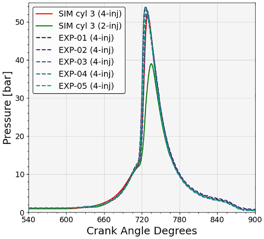
In-cylinder pressure traces for both 2-inj and 4-inj strategy: red solid for 4-inj, green solid for 2-inj, and all dashed curves for five different 4-inj experiments.
The average gas-phase equivalence ratio from the simulations is shown first in Figure 13, where the standard deviation (
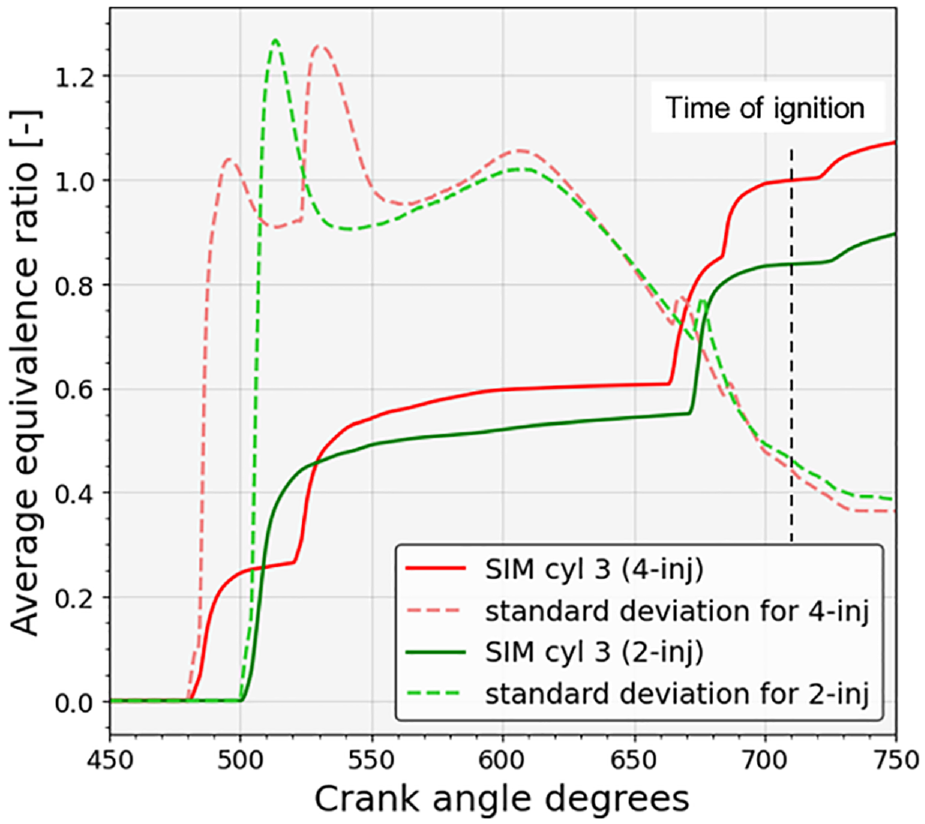
Equivalence ratio in two strategies: red curves for 4-inj, and green curves for 2-inj; solid curves for average equivalence ratio in cylinder, dashed curves for standard deviation of equivalence ratio.
The results of the different injection strategies are shown in Figure 13, where the equivalence ratios increase abruptly right after each injection. The standard deviations increased sharply after each injection since almost all the fuel vapor is first concentrated on the path of the impinging spray, and decreased gradually as the fuel was dispersed with the bulk flow in the cylinder. The fuel-air mixtures became more and more uniform with crank angle, and no big difference was seen between the two strategies from the standard deviation curves at the time of ignition. The main difference was the average equivalence ratio, which was determined by the total evaporated fuel amount. At the time of ignition, the average equivalence ratio was about 1 for the 4-inj strategy, but only 0.84 for the 2-inj strategy; the spatial fuel distribution is presented in Figure 14, where different levels of equivalence ratios for the two strategies are shown. The close-to-one average equivalence ratio resulted in much stronger combustion for the 4-inj strategy.
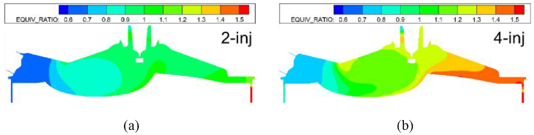
Fuel distribution at the time of ignition: (a) for 2-inj and (b) for 4-inj strategy.
Figure 15 tracks the state of the injected fuel at different crank angles from the early injections all the way to the time of ignition for both strategies, presenting where the injected fuel is distributed in the cylinder. The vertical axis represents the ratio of the corresponding fuel mass to the total injected mass from both/all injections. The gaseous fuel in cylinder is shown in Figure 15(a), and it has exactly the same trend as the average equivalence ratio in Figure 13. The 4-inj curve at around 650 CAD, just prior to the late injection, is very close to 50% which means almost all the fuel from the early injection has evaporated before the late injections, while the lower curve for the 2-inj strategy indicates thicker films on the wall and incomplete evaporation. The trend of the wall wetting can be clearly seen in Figure 15(b): about 34% remains in the films for the 2-inj strategy at the time of ignition, while only 24% for the 4-inj strategy; the majority of the overall wall wetting stems from the late injection(s).
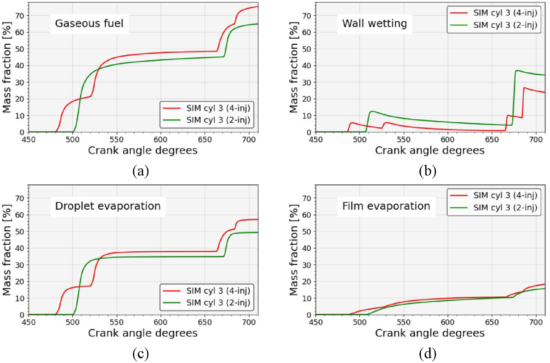
Fuel tracking in cylinder: vertical axis for mass fraction in total injected mass during all injections; red curves for 4-inj, and green curves for 2-inj; gaseous fuel in (a), wall films in (b), droplet evaporation in (c), and film evaporation in (d).
Figure 15(c) and (d) are more interesting, and they reveal more details about the evaporation process. Figure 15(c) shows the fraction of the fuel evaporated from fuel droplets; this includes two contributions, from the fuel spray before hitting the wall and from the droplets in the rebound and splashed portion. Figure 15(d) shows the evaporation from the surface fuel films, which is a gradual and slow process compared to the droplet evaporation, due to a low wall temperature and limited surface area. In both cases, a higher evaporation rate is seen for the 4-inj strategy.
The droplet evaporation, Figure 15(c), is discussed first. Two possible reasons are responsible for the faster evaporation in the 4-inj strategy. We will take the early injection as an example for explanation, and the late injection works in the same way.
As mentioned earlier, the same fuel rail pressure (FRP) was used for these two strategies. Thus, it would be expected that the injection duration for the 2-inj early injection (see alias in Table 2) was approximately the same as the sum of the durations for the first and second injections for the 4-inj early injection (also Table 2). Then the 2-inj early injection could be hypothetically divided into two continuous injections for analysis: the first half equivalent to the first 4-inj early injection, with the second half leading to the differences. In the 4-inj strategy, the time between two early injections was long enough (over 15 times as long as the injection duration) that the evaporated fuel from the first injection would be moved away by the bulk flow from its original location (near the injected spray path), which created a fresher or leaner mixture near the injection path compared to the second half in the 2-inj strategy, thus promoting the evaporation process from the second 4-inj early injection.
The other possible reason was related to the rebound and splashed portion after the fuel droplets collided with the wall. Those rebound and splashed droplets from the first half of the 2-inj strategy were pushed closer to the wall by the second half of the injection and the induced flow fields near the wall, so that more droplets got re-deposited instead of escaping from the wall and ended up contributing to the wall wetting.
Although the differences in Figure 15(d) are small, a higher film evaporation rate can be seen for the 4-inj strategy. To explain this, the late injections are considered first. Figure 16 shows the equivalence ratio distributions at EOI of each injection, where the injection process can be visualized. Table 2 gives the temporal order of each injection: First 4-inj late, 2-inj late, and second 4-inj late from early to late. These correspond with different piston heights: First 4-inj late, 2-inj late, and second 4-inj late from low to high. Thus, the fuel spray would impinge on different locations of the piston bowl. The first 4-inj late hit the right half of the bowl, and the second 4-inj late mainly hit the left part, resulting in a larger wetting area, which accelerated the evaporation process for the 4-inj strategy compared to that for the 2-inj strategy.
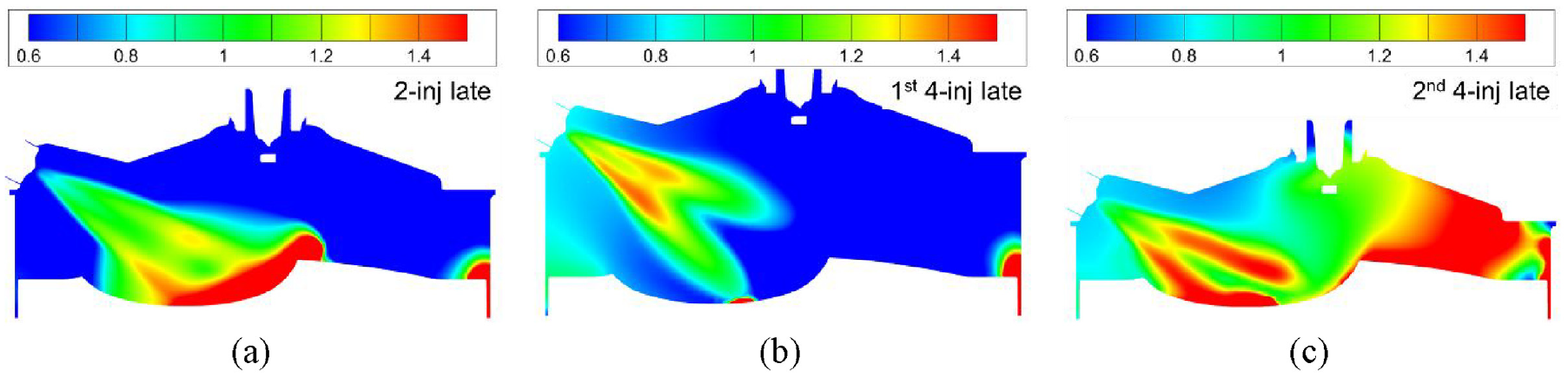
Equivalence ratio distributions at EOI of each injection for different strategies: (a) for late injection in 2-inj strategy, (b and c) for first and second late injection in 4-inj strategy, respectively.
To add to this, the impingements from the early injections using different strategies are compared. The film thicknesses at 10 CAD after each SOI are shown in Figure 17, where the cylinder and the piston geometries are shown as well. These early injections were during the intake stroke, where the piston was moving downwards. Most of the fuel spray in the two early injections in the 4-inj strategy from the 6-hole injector hit the same area of cylinder wall, and only a small portion (lower part) hit different locations, which slightly increased the evaporation area. So, compared to the late injection, the differences for the early injections were even smaller.
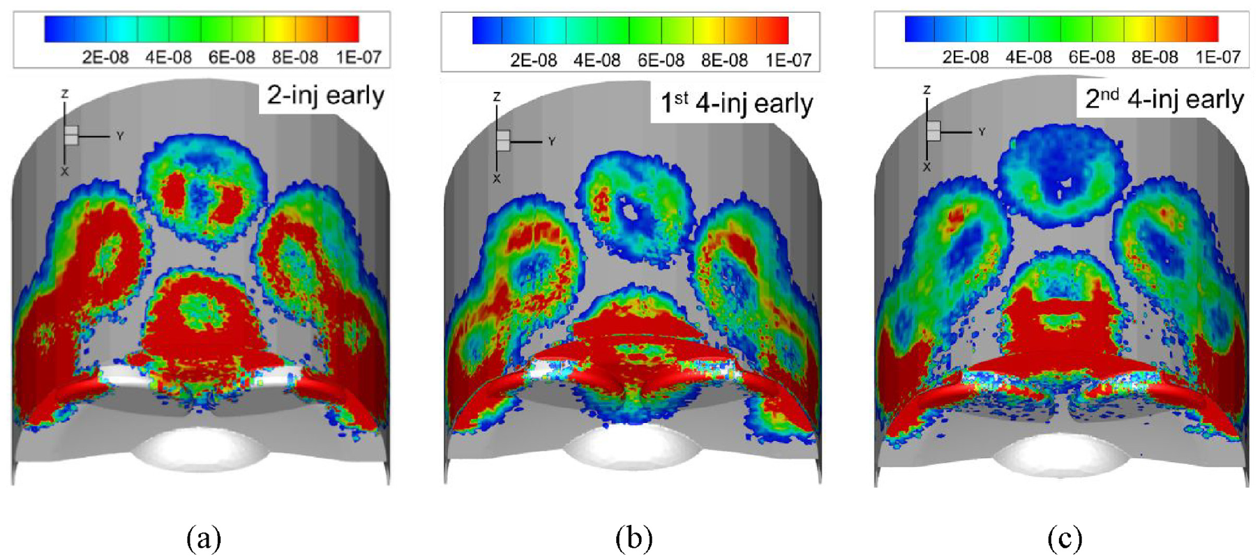
Film thicknesses on the wall at 10 crank angles after each SOI: unit, meter: (a) for early injection in 2-inj, (b) for first early injection in 4-inj, and (c) for second early injection in 4-inj.
The final remarks in this section are related to the effects of the improved strategy on the other three cylinders. Typically, like cylinder 3, the other cylinders also experienced increased amounts of evaporated fuel with multiple injections, resulting in stronger combustion. However, the rapidly increasing engine speed in the improved strategy caused by the stronger combustion in the previous cylinder(s) led to a lower RPM-normalized turbulence intensity during combustion; this had an adverse effect, which was relatively weak but not negligible, compared to the enhancement from the higher average equivalence ratio. A comparison of the engine speeds using the 2-inj and 4-inj strategies is provided as Figure 3 in our previous paper. 14 In particular, for the intake strokes of cylinders 2 & 1, seen in that figure, the engine speed with the 4-inj strategy significantly surpassed that of the 2-inj strategy, enhancing the engine intake turbulence intensity, making a direct comparison of the effects of the normalized turbulence more complicated. Nevertheless, the overall effect is presented in Figure 4 of that same paper 14 : the combustion process for all four cylinders was greatly enhanced in the improved strategy, with the least increase of peak pressure for cylinder 1 (the last one to fire), where the engine speed increased the most.
Summary and conclusions
A multidimensional simulation using the FES model was carried out for all four cylinders of a GDI engine in the very first firing cycle for the cold start process. Rapidly changing transient engine speeds and the low evaporation rate of the fuel introduced extra complexity into the simulations. The in-cylinder pressure traces in the experiments were presented first to provide validations for the FES model, followed by a thorough analysis of the causes for different combustion intensities in different cylinders. An improved 4-injection strategy, was proposed as well, displaying great potential to enhance the fuel evaporation process during cold start.
The primary conclusions from this study are:
Comparing cylinder pressure traces from the experiments for all four cylinders with the FES model, it was able to predict the combustion intensities in different combustion regimes, including the initial combustion, the level and phasing of the peak pressure, and the respective trends in all four cylinders. This verified the capability of the FES model to simulate engine behavior under cold start conditions, which included the transient engine speeds and cold walls.
In the very first firing cycle for the GDI engine studied, very strong combustion was observed for cylinder 3 (peak pressure about 40 bar), which was the first one to fire, while it was relatively weaker and quite similar for the other three cylinders, with peak pressures about 15 bar lower than cylinder 3.
Fuel tracking in the four cylinders indicated that more fuel was evaporated for the first two cylinders to fire due to the quite low engine speed. Also, for the same reason, for these two cylinders, more fuel/air mixture flowed back into the intake ports before IVC. The overall effect was that the mass fraction of gaseous fuel in cylinder for the first two cylinders to fire was very close to the other two cylinders at the time of ignition, around 57%−58% of total injected fuel.
A higher average equivalence ratio due to more injected fuel and a better fuel distribution caused by a higher tumble ratio led to the very strong combustion for cylinder 3, the first to fire. Cylinder 4 (second to fire), compared to cylinder 3, had more non-uniformity for the air-fuel mixture, making the combustion weaker. Lower normalized turbulence made the combustion even weaker for cylinder 4. About 9% less fuel was injected into cylinders 2 and 1 (this is the strategy of the production engine), which caused the lower average equivalence ratio (0.76 and 0.75 in cylinders 2 and 1, respectively, compared to 0.84 in cylinder 3) and thus a lower peak pressure.
An improved strategy was identified, where a 4-inj strategy showed promise to evaporate more fuel from both droplets and films under cold start, resulting in a peak pressure increase of about 15 bar compared to the baseline strategy (about 40 bar peak pressure).
Droplet evaporation was enhanced using the 4-inj strategy. There were two possible reasons: a more dilute mixture near the path of the second early/late injection created a lower fuel vapor pressure environment for evaporation, and the rebounding and splashed droplets from the first early/late injection had a higher fuel mass and more time for entrainment.
For both early and late injections, the 4-inj strategy distributed the fuel that impacted the piston and cylinder over a larger area relative to the 2-inj strategy, which would accelerate the film evaporation process.
An interesting observation related to the large engine speed variations during the cold start is the partial disconnect of the usual linear relationship between turbulence intensity and engine speed that is typical of steady operation. Since the turbulence characteristics are largely set up by the intake process, the turbulence levels at the time of ignition more closely reflect the engine speed during intake and not the engine speed at the time of ignition as reflected in the normalized turbulence intensity seen for cylinder 4, the second to fire.
Footnotes
Acknowledgements
We wish to thank CONVERGE CFD™ for providing us with licenses for their simulation software and for their generous technical support. All the simulations shown in this study would not have been possible without the resources and continued support from the Texas Advanced Computing Center (TACC) of the University of Texas at Austin.
Declaration of conflicting interests
The author(s) declared no potential conflicts of interest with respect to the research, authorship, and/or publication of this article.
Funding
The author(s) disclosed receipt of the following financial support for the research, authorship, and/or publication of this article: This work was financially supported by the Ford Motor Co. through the University of Texas at Austin’s Site of the NSF Center for Efficient Vehicles and Sustainable Transportation Systems (EV-STS).