Turbulent flow development within the discharge cavity of a screw compressor

Abstract

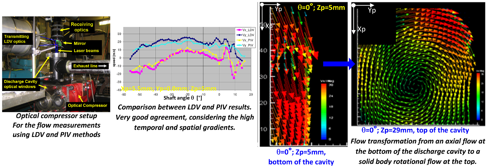
Spatial flow field velocities within the discharge cavity of an optical screw compressor have been measured using LDV and PIV techniques. Angle-resolved velocities were obtained over a time window of 1° at a speed of 1000 rpm, pressure ratio of 1 and temperature of 55°C. Comparison between the LDV and PIV results showed very good agreement and provided a good level of confidence in the presented data. Overall, the flow field results revealed the presence of a complex, turbulent, 3D and vortical flow structure within the discharge cavity. LDV measurements at the exit of the discharge port showed that the inflow into the cavity has two distinct flow features that includes undulated velocity profiles with high gradient during the opening of the port, and uniform jet-like flows during the rest of the time. The energy necessary to create that jet-like flow was from the built-in pressure in the rotors. Turbulence fluctuations were high and followed the mean flow variations with values up to 35% of the mean values during the undulating flow. PIV spatial mean flow measurements showed a uniform axial flow close to bottom of cavity that has been transformed to a stable solid body vortex at the top of the cavity. These measurements within the discharge cavity are made for the first time and they are unique and in great detail that can be used for validation of CFD codes and optimisation of compressors to improve their efficiency for different system applications.

Graphical abstract

Introduction

Nowadays, the use of screw compressors is widespread and has widely replaced the traditional reciprocating compressors with many industrial applications, for example, apart from their regular use in refrigeration and air conditioning systems, they are also commonly used for air compression, engine supercharging, food process, pharmaceutical and pneumatic transport. This is due to their simple design and high efficiency over a wide range of speeds and pressure differences, and more importantly, the development in manufacturing tools which enables new rotor’s profiles to be made with fine tolerances within 3 μm at a reasonable cost.^1,3 The screw compressor used in this investigation was an ‘N’ type rotor profiles with 5/6-lobe configuration which consists of two rotors, male and the female, contained in a casing with no valves and their meshing lobes form a number of working chamber flows (five here) within which compression takes place as described in Stosic. ¹ The compression process continues until the working chamber flows between the rotors (five times within a full cycle) with high pressure are exposed to the discharge port and then flow through the port into the discharge cavity.^2–4

Many studies have been carried out on screw compressor performance, which led to improvement in their design and efficiency for different applications, particularly, for automotive, refrigeration and air conditioning systems.^2–10 The engine performance tests carried out by Matsubara et al. ⁵ confirmed the advantages of using screw compressor supercharger over the four other types of positive displacement compressors (PDC). For an efficient car fuel cell, it has been shown that a twin screw machine can perform both the compression and expansion functions, using only one pair of rotors. ⁶ The suitability of the use of screw compressors for the car air-conditioning systems was also confirmed by Fukazawa and Ozawa ⁷ compared with other PDCs. It has been shown that the efficiency of refrigeration screw compressors is highly dependent on their rotor profiles and clearance distribution. ² A performance predicting model of screw compressors for refrigeration systems has been developed by Liu et al. ⁸ which correlates the running conditions to the design parameters. The use of alternative refrigerants has been investigated and evaluated by Karnaz ⁹ for screw compressors by considering the impact of the refrigerants and lubricants viscosities while the use of various combinations of injection fluids (oil and refrigerants) were investigated numerically and experimentally by Stosic et al. ¹⁰ to evaluate how they affect the compressor efficiency, noise and reliability.

Overall, the predictions of the screw compressors performance, design optimisations and basic operations are well established and known, but there is limited information in the literature on the flow behaviour within compressors. ² A clear understanding of the flow processes is essential as it would greatly help the machine performance and, in fact, their characteristics should be an integrated part of the design and optimisation process of screw compressors.^3,11–13 The flow within the screw compressor can be divided into four sections, from suction to the exhaust. The first is the suction flow that feeds into the second section of five rotors’ working chambers through which the gas is pressurised as it is convicted towards the third section of discharge port, where the flow exits into the last section of the discharge cavity. Thus, it is clear that the flow process within the discharge cavity depends strongly on flow coming from suction to the rotors’ chambers, and then through the discharge port with high pressure difference into the discharge cavity. On the other hand, the flow within the discharge cavity depends also on the physical geometry and confinement of the cavity’s chamber that dictate the flow development within it. Since within a cycle there are five openings of the discharge port, the flow coming into the discharge cavity is expected to be of 3-D, highly turbulent and time dependent nature, which causes variation of mass and pressure pulsations during the discharge process within the cavity.^2,14 Therefore, it is essential to have a full physical understanding of the gas flow motion characteristics within the suction port, rotor’s working chambers, discharge port and the discharge cavity by quantifying the time-resolved mean and RMS velocity variation so as to describe the whole flow sequence of processes.

Previous works on the flow behaviour within screw compressors are scarce, however, there are limited experimental and CFD investigations that measured and simulated flow within the screw compressors. Full details of the flow characteristics within the suction, working chamber and near the discharge ports were measured and already reported in Nouri et al.^15–17 by current authors. This report is the continuation of the same research project, focusing on the turbulent flow behaviours within the discharge cavity by measuring the mean and turbulence velocities using LDV and PIV techniques. Although limited, a good number of CFD flow simulations have been made in screw compressor, especially those that are capable of handling single and multiphase fluids.^11,18 The suction flow was simulated by Arjeneh et al. ¹¹  and Mujic et al. ¹³ and it was concluded that the flow losses in the suction port would lead to a decrease in compressors efficiency. ¹³ The simulation by12 has shown that the suction port shape and the inflow trajectory into the rotors’ chambers would influence the flow within the rotors. The investigations of Stosic ²  and Pascu et al. ¹² have shown that the use of new techniques for rotors profiling helped to manufacture rotors of complex shapes with tolerances of the order of few microns, which improved efficiencies. Also, a limited number of the previous investigations have been carried out^19,20 to characterise flow leakages using experiments and CFD simulations. The gas pulsations are also a main source of noise within the discharge cavity and have been investigated since 1986 by many authors. For example, the gas pulsation, vibration, and noise were measured first by Fujiwara and Sakurai, ²¹ and then an acoustic model was developed by Koai and Soedel^22,23 who showed how the low pulsation is related to the compressor performance.

As described above, the flow in screw compressors is complex, 3-D and strongly time-dependent similar to the in-cylinder flows in automotive engines,^24,25 centrifugal pumps, ²⁶ turbocharger turbines, ²⁷ wind turbines, ²⁸ mixing reactors, ²⁹ geothermal power plants, ³⁰ Slot-Die Melt Blowing ³¹ and many other applications in combustion and heat transfer. This implies that the measuring instrumentation must be robust to withstand the unsteady aerodynamic forces, have high spatial and temporal resolution and, most importantly, must not disturb the flow. Only optical diagnostics, particularly LDV and PIV, can fulfil these requirements to characterise turbulent flow structure in detail, as demonstrated by previous research in similar flows. The recent work of Koca and Ozturk ³² on a spirals cylinder surface successfully used PIV to measure mean and RMS velocities, turbulent kinetic energy (TKE) and Reynolds shear stress (u′v′).

The main objective of the current research work is to measure the real time flow dynamics within the discharge cavity chamber. To the authors’ knowledge, there has been no attempt to measure the gas flow characteristics within the discharge cavity and the data presented in this report is original and a unique contribution to the literature. The new measured data has been obtained in great detail to be used for the validation of CFD codes to establish a reliable model for accurate prediction of flow and pressure distribution within twin screw machines, which can then be used as a tool to further improve the design of screw compressors and expanders. Current measurements were performed at the exit of the discharge port and within the discharge port cavity using LDA and PIV systems by passing the laser beams and sheet through specially designed transparent windows, made of Plexiglas (Perspex), that were installed on the compressor casing at two ends of the cavity chamber without altering the physical integrity of the cavity’s internal geometry. The optical details will be given in the following section where the flow configuration is given. The results will be presented and discussed in the subsequent section and the report will end with a summary of the main findings.

Flow configuration and instrumentation

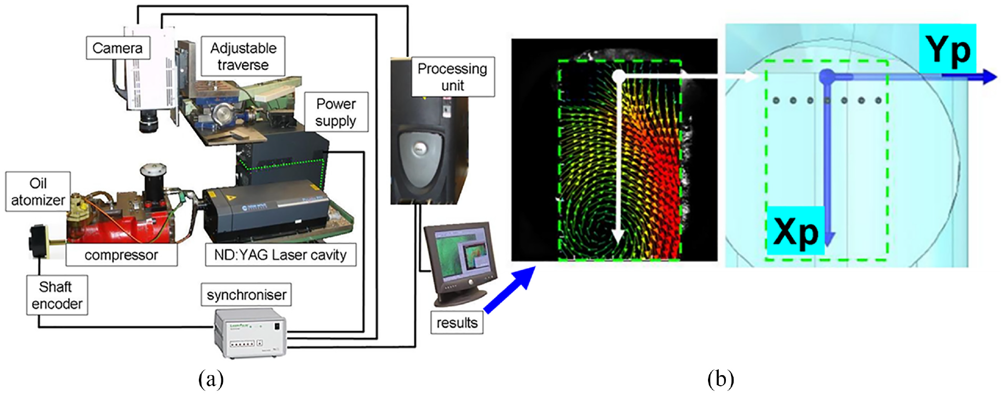
LDV and PIV systems were used to measure mean and RMS velocities and instantaneous planar velocity vector within the discharge cavity of a screw compressor. The LDV and PIV techniques are well established and the systems used were the same as those used by Refs.^{3,15,16,25,27} who described the LDV and PIV systems in full detail (including all related errors and uncertainties) which will not be repeated her, however, detailed summaries of both methods are provided below. The test rig was modified to accommodate the optical compressor, LDV/PIV transmitting and collecting optics, and their traverses. Special attention was paid at the location of the optical windows and their design according to recommendations made by Arcoumanis et al. ²⁷ To allow sufficient optical access, two fully polished flat transparent windows were fixed at the end of the discharge cavity and on the top of the T-junction of the exhaust line as shown in Figure 1(a) with the LDV optical set up. With this arrangement, no change has been made to the internal profile of the cavity. Transmitting and receiving optics are located on the top of the T-Junction window, as shown in Figure 1(a), and the laser beams are directed into the discharge cavity via a 45° mirror to form the measuring control volume (CV). The photomultiplier (PM) of the receiving optics is also positioned near the top window next to the mirror, and it is aligned carefully to be focused onto the measuring CV to ensure only the light scattered from tracers crossing the CV is detected. The PM comprised collimating and focusing lenses with a 100 μm pin hole to give an effective measuring CV of 79 × 79 × 100 μm. The PM was positioned at approximately 22° ± 3° to the full backscatter configuration. Data from PM was collected continuously with respect to shaft rotation, θ, until sufficient samples were collected. The samples were then processed to obtain averaged mean and RMS velocities over 1° time window; a sample of processed data is shown in Figure 1(b).

Figure 1.

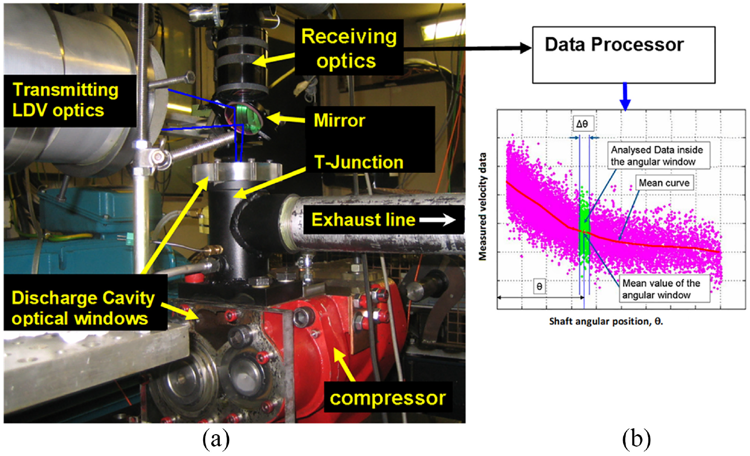
(a) Modified optical compressor with two transparent windows and the LDV optical system set up and (b) a sample of angled-window resolution for averaging mean and RMS velocities.

The silicon oil droplets with average size of 1–2 μm were used as the flow tracer for both LDV and PIV techniques and it was shown to be suitable, in particular, for PIV^3,25 measurements, which allowed good data processing when using the cross-correlation method. The main disadvantage was the fouling of optical windows occurring after 20–25 min of continuous running; this suggests that care must be taken to clean the windows regularly. Also, a shaft encoder attached to the compressor shaft is used to synchronise the angular position of the rotors to the measured LDV/PIV data (as they are obtained over several cycles) and for the post processing and analysing of the results.

Figures 2 and 3 show the discharge port and cavity flow geometry and the adopted coordinate system for LDV/PIV measurements. The pressurised fluid within the rotor’s chambers is forced through the discharge port (during its opening and closing) and moves into the discharge cavity. Before going into further detail, a description of the complex flow geometry of the discharge is required to better understand the measured flow behaviour. The discharge chamber is divided into two parts, the discharge port and the discharge cavity. First, the discharge port flow passage that connects the rotor’s chambers to the discharge cavity. From the Figure 3, it is clear that the discharge port is a converging flow path where the cross-section area gradually reduces as the flow moves through the port from the W-section (on the rotor side with a cross-section shaped like a W) to the V-section (on the cavity side with a cross-section shaped like a reversed delta or V, similar to the shape of the discharge cavity), causing the flow to accelerate through the port before entering into the discharge cavity. Secondly, the discharge cavity with much larger volume than the port, also has a complex shape similar to a heart (or V) with its apex at the bottom of the cavity and its top connected to the exhaust pipe, see Figures 2(a) and 3(b). Considering the above flow feature and also the fact that there is simultaneous overlapping of five rotor’s working chamber flows (during a full cycle) within the discharge cavity, ¹⁴ the expectation would be that the flow exposure into the cavity chamber is of a complex nature of fast moving, highly turbulent and time dependent flow, which in turns influences drastically the mean velocity profile development and distribution within the discharge cavity. A representation of convergence from W- to V-section of the port, and a schematic mean flow through the discharge port and its exposure into the cavity are also shown in Figure 3(b). In addition, another flow feature that can influence the flow through the port and also into the cavity is when the high-pressure flow from the rotor’s chamber moves into the port (at W-section) during the port opening and closing as explained by Nouri et al. ¹⁶ The position of the discharge port is fixed and the opening and closing of flow is controlled by the end face of the male and female rotors and therefore the process is a gradual opening and closing depending on the angular positions of rotors. Thus, the flow exposure (or mass flow) to the port varies as θ changes, which can have considerable control on flow velocity trajectory and distribution in discharge port and cavity, see Nouri et al. ¹⁶ for more details.

Figure 2.

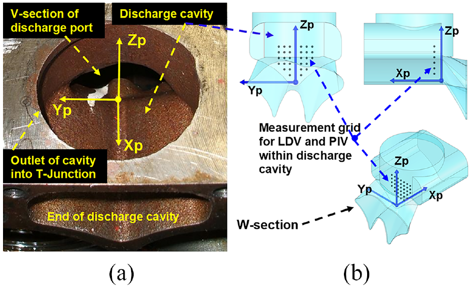
Coordinate system within the discharge cavity: (a) physical geometry of the discharge cavity chamber and (b) the adopted coordinate system at different cross-sectional planes with the grid for LDV measurements.

Figure 3.

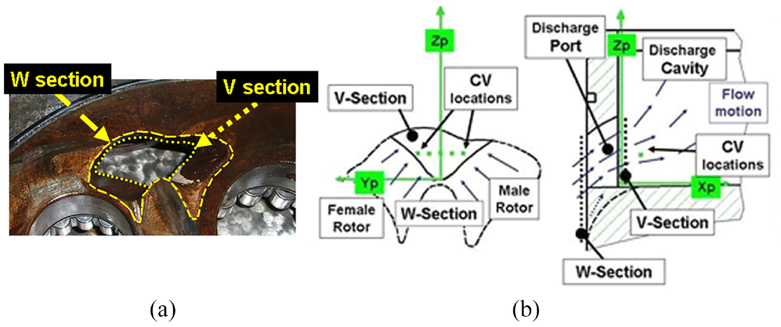
Discharge flow setup: (a) picture of the W-section and V-section and (b) Coordinate system inside the discharge cavity and a schematic representation of mean flow velocity within the discharge chamber.

In order to describe the flow domain properly for such a complex flow and geometry (described above), it was decided that the best coordinate system is the one identified with reference to the port by the axes Xp, Yp and Zp, with its common origin placed at the bottom of the cavity at the V-section as shown in Figures 2 and 3, where the positive direction of all three axes are also shown. LDV measurements have been taken at one axial location, Xp = 5.5 mm, that is, 5.5 mm into the discharge cavity from the V-section (exit of the discharge port), for different Zp and Yp locations within a measurement grid in the Yp-Zp plane covering the V-section area, as shown in Figure 2(b). This Xp location was as close as to the V-section that our LDV setup allowed and characterises the flow entering (inflow) the cavity from the port. LDV measurements include angle-resolved (over Δθ = 1° of the shaft rotation) mean and RMS velocities of axial (Vx, along Xp) and horizontal (or transverse, Vy, along Yp) components. Although LDV measurements provide very accurate information about mean and RMS velocities, it is a point measuring system and to describe the flow characteristics across all fluid domains in full detail it would be very time consuming. PIV system is an alternative measuring technique that can capture instantaneous flow field velocity vector (2-D or 3-D) in a plane and would provide useful information regarding spatial gradient and Reynolds stress everywhere within the measuring plane. Therefore a 2-D PIV system has been used to map the flow within the discharge cavity, and in order to validate the accuracy of the measured PIV data, a comparison between LDV and PIV has been made to provide confidence in the measured data. A summary of the PIV setup is given below; again, full details of both techniques have been given by current authors in Guerrato ³ and Nouri et al. ¹⁶ and will not be repeated here.

The transmitting PIV system comprised a solid-state Nd:YAG laser (high repetition of up to 10 kHz and double pulsed with high energy stability less than 1% of the laser power) and an optical system of cylindrical and spherical lenses to produce the laser sheet; the laser produces green light (wavelength of 527 nm) with a diameter of 1.5 mm and energy per pulse of 10 mJ. The laser sheet was passed horizontally (in the Xp-Yp plane) through the flat window fixed at the end of the discharge cavity and the images were collected through the window on the top of the T-junction using a high-speed camera (Photon FASTCAM-APX) that was fixed at 90° to the laser sheet, as shown in Figure 4(a). The transmitting laser and recording camera were placed on a common 3-D adjustable traverse. With this arrangement, only the components of the mean and RMS velocities in the laser sheet plane (in the horizontal Xp-Yp plane) can be measured, that is, the axial component (Vx along Xp direction) and transverse component (Vy along Yp direction). No measurement could be done for the third direction parallel to Zp, as explained below. The recorded images were passed to the processing unit where the data was analysed and processed using cross-correlation method; a typical sample of the measured mean flow field velocity is shown in Figure 4(b). Theoretically, by swapping the camera and the laser sheet positions, it is possible to analyse flow in the vertical plane, Yp-Zp (where Vy and Vz can be measured), but unfortunately images captured by the camera through the window at the end of the discharge cavity were not clear due to window fouling and therefore were not processed. Also, to avoid laser sheet light reflection from the metal surface of the cavity, the internal surface of the cavity has been painted matte black which reduced drastically the scattered light from the wall.

Figure 4.

(a) Schematic presentation of the PIV optical arrangement and (b) a sample of processed output of the mean flow field velocity vector in Xp-Yp plane.

Results and discussion

The following results are a sample of data obtained in this experiment that show the behaviour of the mean axial and transverse velocity components and their corresponding RMS velocities as a function of the shaft angular position, θ, within the cavity; full set of results are presented in the thesis of Guerrato. ³ It should be noted that the LDV and PIV results presented here cover only 72° of the main shaft rotations, which corresponds to one full opening and closing of the discharge port, out of five, during a full rotational cycle; the flow over the other four rotor’s chambers are considered to be the similar. Here, in all presented results, the opening of the discharge port corresponds to the main shaft angle of θ = 0° and is the same for both LDV and PIV measurements.

LDV results

The velocity profiles depicted in Figure 5 are obtained from continuous measurements with respect to shaft rotation over many cycles until sufficient samples are collected to provide accurate (statically) mean and RMS velocity over a 1° time window. The graphs on the left column of Figure 5 represent the mean axial velocity (Vx), while those on the right column are the mean transverse velocity (Vy) profiles. All results were obtained at Xp = 5.5 mm for three Yp (−8, 0 and +8 mm, with Yp = 0 mm coincident with centre of the V-section) locations; the graphs at each given Xp and Yp locations, contain velocity profiles at different Zp locations of 5, 9, 13, 17, 21 and 29 mm, with Zp = 5 mm close to bottom of the discharge cavity and Zp = 29 mm near the top of the cavity. The flow at this Xp location for different Yp and Zp can be considered to be the inflow from the discharge port into the discharge cavity.

Figure 5.

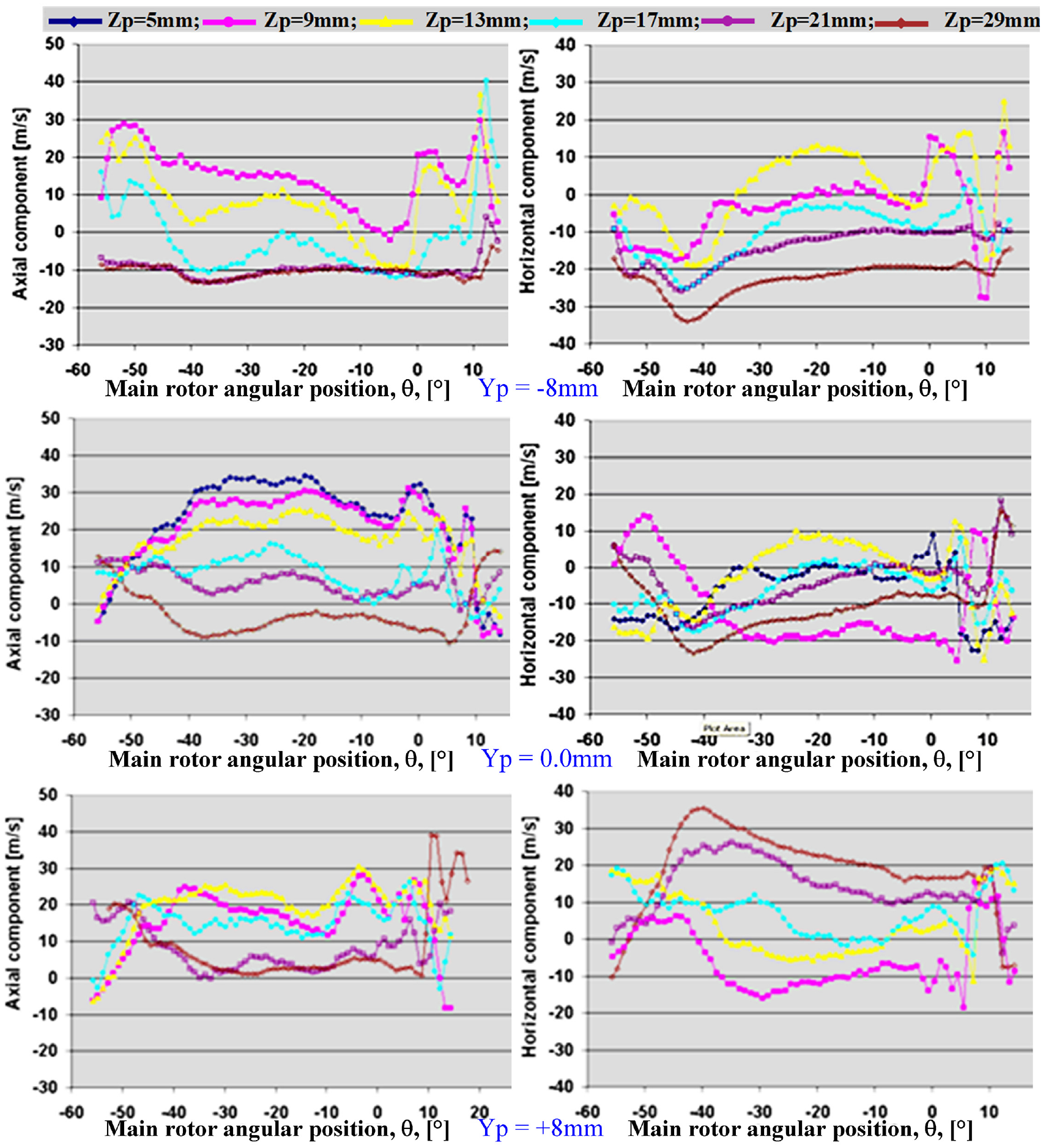
Axial and transverse mean velocity distributions as a function of main shaft angular position, θ, at Xp = 5.5 mm, the inlet of discharge cavity, at different Zp and Yp locations as indicated on the graphs.

In general, the axial (inflow, left column) velocity profiles of all graphs in Figure 5 at all Yp locations show a common trend that can be divided into three parts: a plateau (uniform) profile which takes place in the centre of the graphs (θ = −40° to 0°), and two wavy (undulated) parts that appear at the extremes of each graph. The results of main uniform jet-like flow show that Vx velocities are always rising as Zp decreases, with the highest velocities at Zp = 5 mm (near the bottom of the cavity), and the lowest velocities (even negative, back flow) at Zp=29mm and Yp = −8 mm (near the exhaust pipe). Also, there are distinct differences in the uniform parts of the flow with Yp locations when moving from the left (−Yp, male rotor) to the right (+Yp, female rotor) side of the cavity due to the asymmetric shape of the V-section of the port, with the highest axial inflow into the cavity occurring at Yp = 0.0 (middle row of Figure 5 for Zp = 5–17 mm), which coincides with the middle of the V-section. However, on the left of the port at Yp = −8 mm, near the top of the cavity (top row for Zp = 21–29 mm), the axial velocity measurements, Vx, exhibit negative values. This suggests the presence of a flow recirculation around the top of the cavity chamber, while on the right side at Yp = +8 mm (bottom row for Zp = 21–29 mm) the axial velocity, Vx, results show the fluid is almost static. The energy necessary to create that central jet-like flow is given by the difference between the built-in pressure within the rotors’ working chambers and the ambient pressure of the discharge port. The results showed that the jet-like flow has strong spatial and temporal gradients that would cause a highly turbulent motion as it moves inside the discharge cavity.

On the extremes of each graph, the results clearly show a rapid variation in the mean velocity profiles, which is directly linked with the opening of the discharge port (θ= 0°), so that the velocities start to fluctuate right after and during the opening of the port up to θ = 15° for both components and for all measured positions. While the wavy shapes on the extreme left of the graphs are nothing but the propagation of the perturbation of the flow caused by the opening of the port which happened (θ = −57° to −40°) on the closing of the previous rotor’s working chamber. Thus, the wavy behaviour of the mean velocity profiles occurs during the opening of the port and is due to the initial pressure difference and the overlapping of closing and opening flow structure from consecutive working chambers. However, at a certain angular location (at around θ= −40°) the opening effects diminish, and it is replaced by a smoother (uniform) pressure distribution and therefore the formation of the plateau flow that was already mentioned. That is to say that the inflow into the cavity is driven directly by the change in volume of the connected rotors’ working chambers. In fact, those chambers act as a piston that pushes the air out of the working chambers giving high axial velocities which are predominantly positive.

Similar flow structure can be seen with the transverse flow (horizontal component in the right column of Figure 5), which maintains a central zone with relatively uniform profiles and the two wavy shapes at the extremes end of the graphs. Despite the similarity in profiles, Vy velocity behaves in a completely different manner to those of Vx in terms of velocity magnitudes and directions. In fact, Vy velocity values at Yp = −8 mm are mainly negative, particularly on the upper half of the cavity (Zp = 13–29 mm) with velocity as high as −35 ms⁻¹ at Zp = 29 mm. As the measuring points move towards the right side at Yp = 0.0, the flow goes through a transition with partially negative and partially positive flow velocity, with no clear correlation between measuring locations and velocity magnitude. However, further to the right at Yp = 8 mm, the flow becomes more positive with a jet-like profile and velocity of up to 35 ms⁻¹ at Zp = 29 mm. This suggests that as the inflow enters into the cavity, the transverse flow tends to converge towards the centre of the cross-section area. This comment is also supported by the fact that despite the irregular shape of the discharge port, it is a converging channel directing flow towards the centre.

Figure 6 represents the axial and transverse turbulence velocity fluctuation profiles as a function of the shaft angle and each set of graphs contain RMS velocity profiles at Xp = 5.5 mm, Yp = 0.0 and at different Zp, and correspond to middle row mean velocities of Figure 5; the results at Yp = −8 mm and +8 mm are not presented due to similar behaviour to those at Yp = 0.0. In all presented graphs, turbulence appears to be around 15% of the mean velocity during the uniform flow part, while it increases up to 35% during the wavy parts, and it seems to be independent of the component chosen. As for fluctuation of the RMS velocities, they do follow the mean velocity variation and are highest at the deepest velocity gradient, especially during the opening of the port where the temporal and spatial mean velocity gradient are the strongest. The RMS velocity profiles presented in the graphs of Figure 6 can be divided into three parts, like that observed with the mean flow of Figure 5. First a central zone, where turbulence is almost constant or changes gradually and uniformly towards the opening of the port, while the turbulence changes rapidly according to the mean flow variation within the two extreme parts of the graph. A similar trend in the turbulence variation can be seen at Yp = −8 mm and Yp = 8 mm planes with uniform turbulence level in the central region, which is expected as the mean flow in this region is fairly uniform, and high turbulence during the undulated parts (high velocity gradient) after and during port opening. Moreover, in the Zp direction for locations higher than Zp = 17 mm, the turbulence levels are generally lower in agreement with the mean velocity results found in this region where the mainstream of the flow seems to be very low or absent. While at locations lower than Zp = 17 mm (where the mainstream flow is strong) the results show higher turbulence levels within the central region but not uniform. In fact, all curves exhibit a variation trend of 5%–10% in magnitude and those trends seem not to be related to the chosen measuring positions. This suggests that the inflow entering the discharge cavity cannot be considered as a fully developed uniform high-speed turbulent flow, but a mixture of jet-like structure and low speed fluid flow that was already present within the discharge port (from the previous opening of the port), which is dragged into the discharge cavity.

Figure 6.

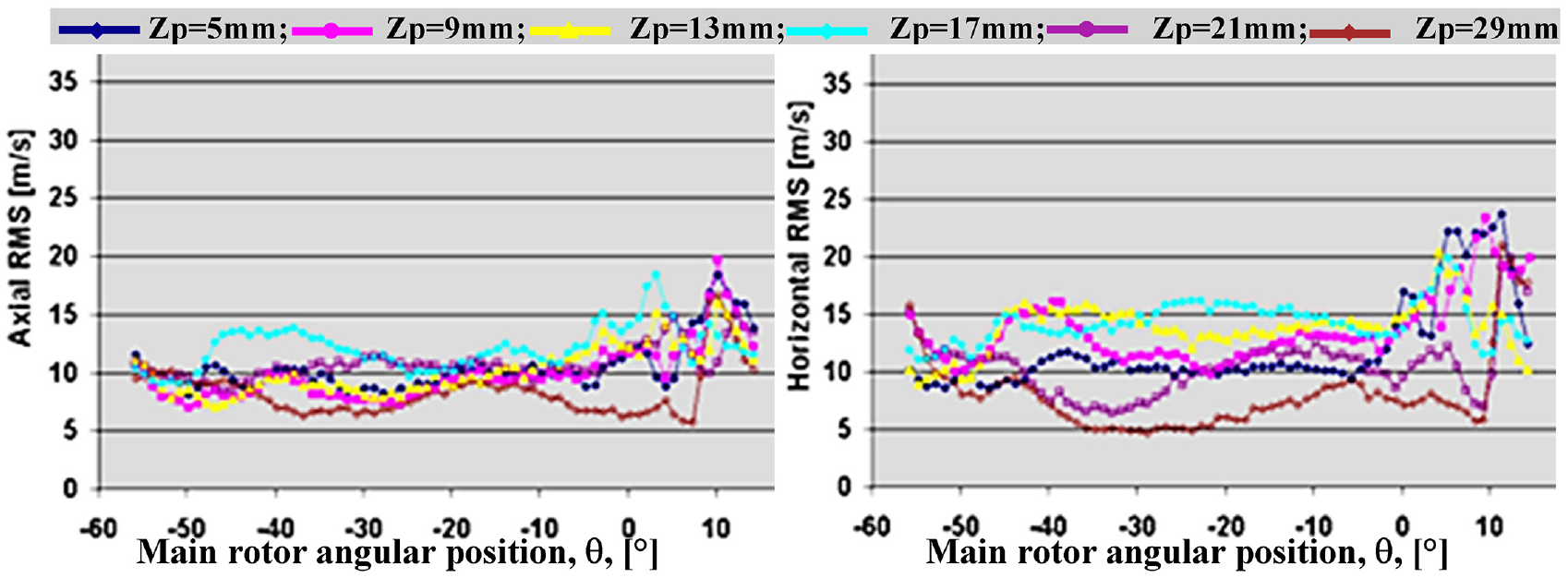
Turbulent axial and transverse RMS velocity distributions as a function of main shaft angular position, θ, at Xp = 5.5 mm, the inlet of discharge cavity, at Yp = 0.0 and different Zp locations as indicated on the graphs.

PIV results

In order to produce consistent results, several measurements were recorded on the same plane and over many shaft cycles. Then, velocity results were averaged to acquire the magnitude of the velocity vector within the cavity over a time window of 1°. Here, 30 images were used to form the mean velocity vector field with an average standard deviation of 10% about the mean value in accordance with LDV results. This is an acceptable result considering the highly turbulent and periodic nature of the discharge cavity flow. Figures 8 to 10 present a sample of PIV measurements of mean flow. Before discussing them, it would be good to present a comparison of PIV and LDV results. As an example, Figure 7 presents such comparison between LDV and PIV results of Vx and Vy velocities at the middle of the discharge port. The results show that both techniques provide similar mean velocity results at most angular locations, θ; this gives a good level of confidence in the PIV presented data in Figures 8 to 10. However, discrepancies still exist with maximum differences of up to 20% at some angular locations, particularly after the opening of the discharge port where the temporal and spatial mean flow gradient are largest. This can be due to statistical uncertainties since averaging over 1° is done over 30 samples, compared to those of LDV with at least few thousand samples.

Figure 7.

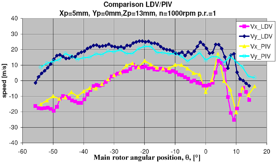
Comparison between mean axial and transverse velocity components obtained from LDV and PIV measurements at the middle of discharge port at Xp = 5.5 mm, Yp = 0.0 and Zp = 13 mm.

Figure 8.

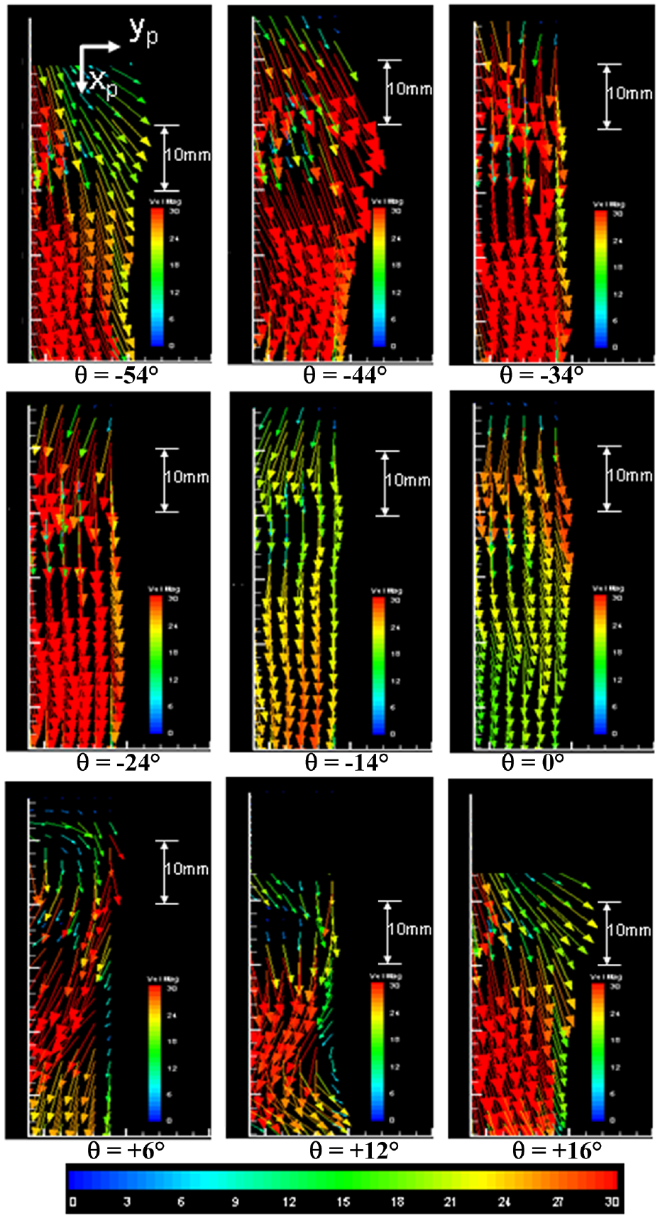
PIV measurement, velocity vector distributions of Vx and Vy as a function of main shaft angular position, θ, at Zp = 5 mm near the bottom of discharge cavity.

Figure 9.

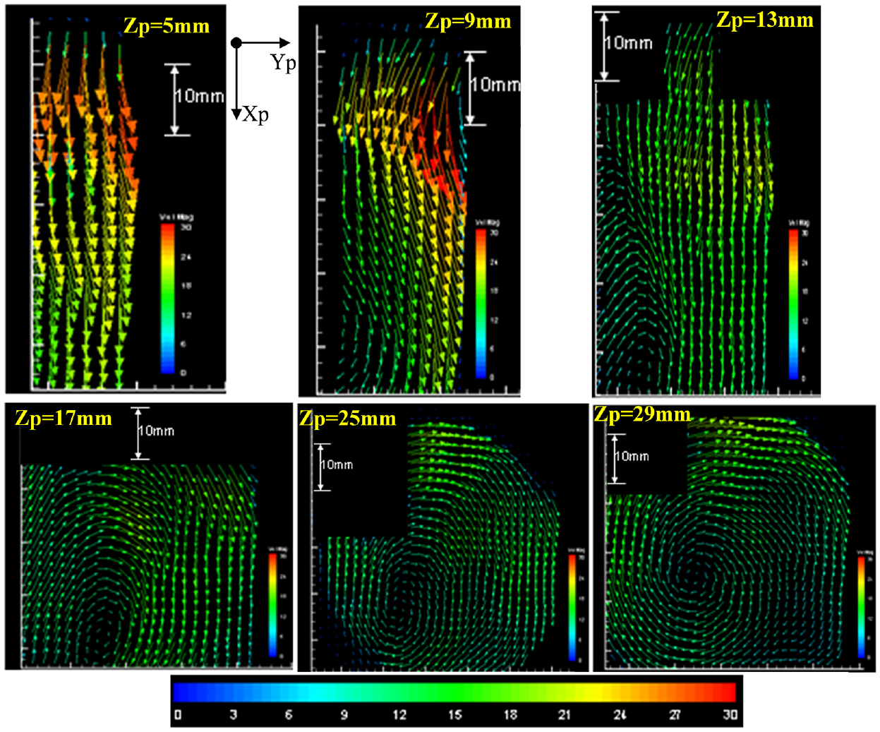
PIV measurement, velocity vector distributions of Vx and Vy at the opening of the discharge port, θ = 0°, and at different Zp locations within the discharge port as indicated on images.

Figure 10.

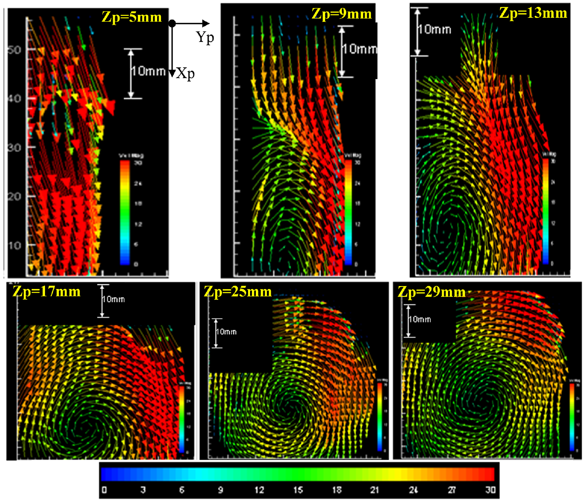
PIV measurement, velocity vector distributions of Vx and Vy during the time when the discharge port is open at θ = −40°, and at different vertical, Zp locations within the discharge port as indicated on images.

Figure 8 shows the angle-resolved of the velocity vector magnitude $\left(\sqrt{{V_x}^2+{V_y}^2}\right)$ of axial and transverse velocities on the Xp-Yp plane at Zp=5mm, near the bottom of the cavity, and at different θ; note that the magnitude of velocity vectors in Figures 8 to 10 are coloured according to the given scalar bar, and the flow scale is given on the Figures. In general, the results show that the dominant flow velocity at all time is mainly in the axial direction (Vx along Xp direction) with a relatively high magnitude at the flow entrance into the discharge cavity. This is especially noticeable from θ = −44° to θ = −24° where the port is fully opened. During the early opening time of the port (θ = +6° to θ = +16°), there is a strong tendency of flow deflection towards the positive direction of Yp with the highest gradient and magnitude of Vy at θ = +12° and θ = +16° at around Xp = 10 mm. This suggests the presence of a transverse pressure wave, originated through the discharge port causing the flow deflection which is controlled partly by the change of the port geometry (from W-section to V-section) and partly by the male and female rotors that influence the flow trajectory within the discharge port. This flow feature will be more evident at higher Zp locations, where it causes the formation of a dominating swirling flow. It is worth noticing that this kind of feature can be captured only by PIV systems with a good spatial resolution.

It is also evident that during the time between θ = −34° up to θ = 0°, the initial pressure gradient is absent, as would be expected due to loss of the flow intensity with lower velocity vector magnitudes, more so at θ = 0°, causing the flow to become mainly in the axial direction with uniform profile in Yp direction. These results are in accordance with those found with LDV where the undulated flow with strong gradient after opening of port, become uniform flow later on. The results also show that as the flow is convected downstream, along the Xp, its intensity reduces gradually due to the fact that the flow is encountering the wall at the end of the cavity and conforms itself to the new physical surrounding, which forces the flow to become increasingly vertical as the end cavity’s wall approaches. It is also due to more flow exposure to the exhaust pipe with Xp. Consequently, the projection of the velocity vectors on the PIV plane (Xp-Yp) becomes increasingly smaller; these can be seen more clearly in Figures 9 and 10 where the flow field at different Zp (from bottom to top of cavity) at θ = 0°and θ = −40°, respectively, are presented and discussed.

The velocity vector results shown in Figure 9 exhibit the horizontal flow field at the opening of the port, θ = 0°, at different Zp. Near the bottom of the cavity at Zp = 5 mm, flow (like shown in Figure 8) is mainly axial along Xp with uniform profiles, small transverse velocity and little spatial gradients; also, a small reduction in the magnitude of the velocity vector can be seen with Xp. At Zp = 13 mm, the first noticeable change compared to that at Zp = 5 mm is a clear reduction of axial flow velocity vector magnitude everywhere, especially along Xp, and more importantly the results show the formation of a recirculation zone at the bottom left corner. Further up around the middle of the cavity, Zp = 17 mm, the results show a further reduction in velocity vectors and that the inflow into the cavity has been deflected right along the Yp and then deflected back to the left further downstream, forcing the flow to form a clear flow recirculation with its centre near the end of the cavity at around Yp = 15 mm. This is expected due to the flow mixture within the cavity chamber of the high-speed jet-like flow with the low-speed flow coming from the discharge port, as explained above with LDV results, and more importantly due to imposed cavity’s boundary conditions as the flow moves through the cavity towards the exhaust. These flow transformations continue as Zp increases with the velocity vector decreasing gradually while the formation of the flow recirculation becomes increasingly developed, so that at Zp = 29 mm near the top of the cavity close to the exhaust pipe, a stable recirculation flow like a solid body rotation flow is formed, with its centre close to the centre of exit pipe at this Zp location. The reduction of velocity vector at this location (Zp = 29 mm) is considerably lower than those at Zp = 5 mm, which is mainly due to flow transition from horizontal to vertical planes as the flow tends to direct itself towards the exhaust pipe.

The results of velocity vector of Figure 10 show similar flow transformation (to that of Figure 9) at different Zp and at θ = −40° when the discharge port is almost fully open with much higher flow velocity vector, which is expected as the incoming flow through the port into the cavity chamber is much stronger and corresponds to the jet-like uniform velocity profiles presented in Figure 5. At this time, unlike that at θ = 0°, the flow deflection starts nearer the bottom of the cavity at Zp = 5 mm and starts to develop a recirculation region at Zp = 9 mm near the end of the cavity. This recirculating flow has been developed further at higher Zp so that at Zp = 17 mm, around the middle of the cavity, a strong recirculation zone is formed with its centre shifting gradually towards the centre of the cavity. This flow transformation continues to develop further with increase in Zp and at Zp = 29 mm; the results show a strong and stable recirculation flow like that seen in Figure 9, but with much higher velocity vectors and that its centre has been shifted almost close to the centre of the cavity. Also, the gradual reduction of velocity vector with Zp is also evident in Figure 10 and as explained before, is due to flow alignment with cavity’s boundary as it is approaching the exhaust pipe. It should be noted that in images of Figures 8 to 10, at all Zp, there are small rectangular black regions within the measuring domain that are shown in dark black. This is due to the incident of the laser sheet on the wall boundary of the cavity chamber, which produced high intensity laser light scattering, despite the use of the matte black paint. This has caused the saturation of signals and made it difficult to detect and process them; due to the high level of noise and inconsistency, the processed data in those areas were removed.

Overall, the PIV results within the discharge cavity highlighted detailed mean flow structure with such good temporal and spatial resolutions, that the LDV approach was unable to provide. On the other hand, as mentioned before, the data sampling for the PIV measurement is smaller than those with the LDV, which makes it difficult to capture fully the turbulence structure with high accuracy. Therefore, the combined LDV/PIV measurement allows a better flow analysis for such a high transient, turbulent and unsteady flow within the discharge cavity. Nevertheless, a sample of axial and transverse velocity fluctuations are presented and discussed in Figure 11.

Figure 11.

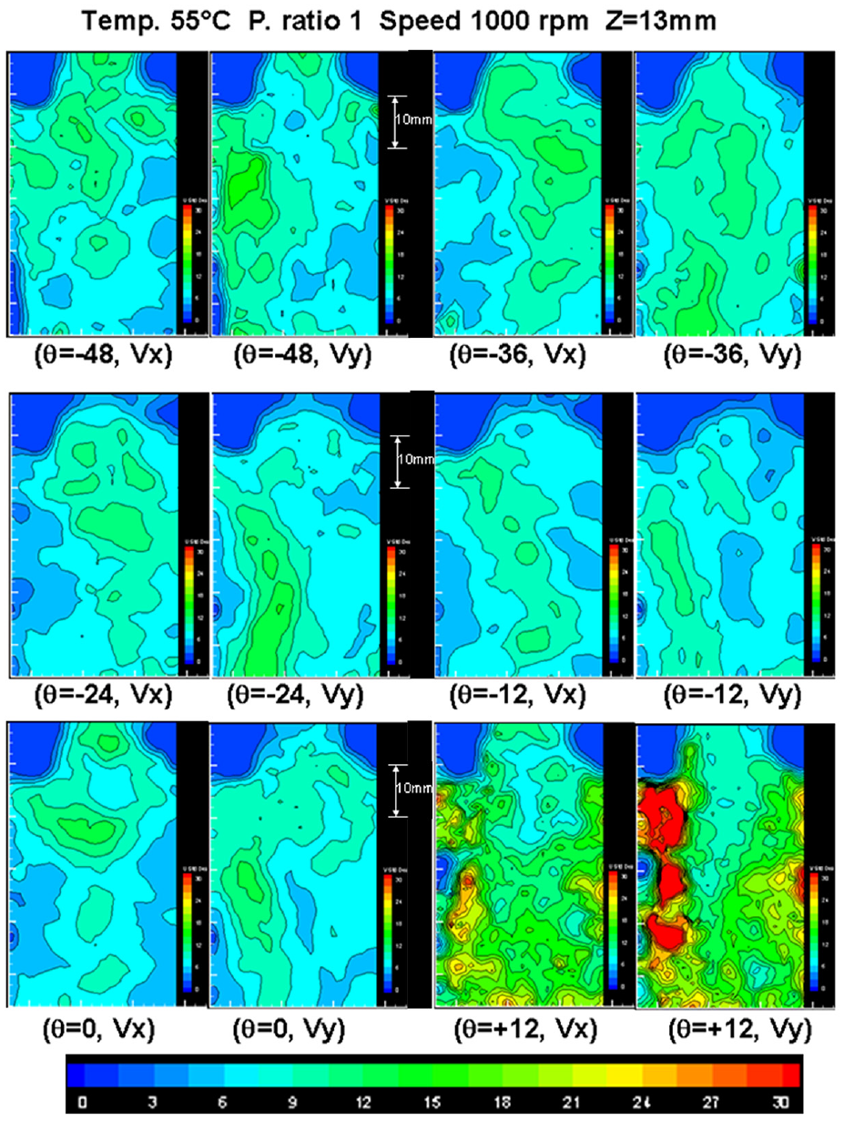
PIV measurement, contours of axial (Vx) and horizontal (Vy) RMS velocity distributions at different θ before and after opening of the discharge port as indicated in the caption of the images, at Zp = 13 mm.

Figure 11 shows the distribution of the turbulence level for axial (Vx) and transverse (Vy) velocity fluctuation components at different shaft angles, θ, at Zp = 13 mm; the velocity magnitudes are according to the given scalar bar, and the flow scale is given on the Figures. The overall results indicate low turbulence RMS values of up to 15 ms⁻¹ at the start of the opening time of the port (θ = 0°) and then they increase with very strong spatial gradient at the early opening of the port (θ = +12°) with RMS values as high as 30 ms⁻¹, especially with the transverse, Vy, component. The high RMS values correspond to large variations in mean velocities observed as wavy profiles from LDV measurements of Figure 5. During the time when the port is fully open (from θ = −48° to θ = −24°), the results show relatively low turbulence (up to 15 ms⁻¹) compared to that of early opening of the port, however, there are small differences between Vx and Vy RMS distributions which follow the mean flow distributions as presented in Figures 8 to 10. The overall results are found to be within the range of the LDV results.

Conclusion

Mean flow velocities and the corresponding turbulence fluctuation velocities have been measured within the discharge cavity of a standard new designed optical screw compressor using LDV and PIV techniques. Time-resolved velocity measurements were made over a time window of 1° at a rotor speed of 1000 rpm, a pressure ratio of 1 and a gas temperature of 55°C. The application of LDV and PIV systems was found to be very successful and offers a novel approach for characterising the flow variation in the optical screw compressors. A summary of the main findings of this research programme are given below:

• LDV mean velocity, Vx and Vy, measurements revealed the presence of a complex flow with velocity profiles commonly divided into three parts: a uniform main part during the time when the discharge port was open, and two wavy and undulated parts that appear at the extremes of each profile after and during the opening of the port. The wavy flow behaviour created strong mean velocity peaks, due to a large pressure gradient, with steep temporal and spatial gradients, while the uniform (jet-like) flow after the rotors opening was due to smoother high pressure builtup with highest velocity close to bottom of the cavity, which gradually decreased towards the top of the cavity.

• Turbulence velocity fluctuations changed according to mean flow variation in all three mean flow parts. On average, the RMS results showed the turbulence level of up to 15% of the mean velocity during the uniform flow part, while it increased to up to 35% during the undulated mean flow.

• Comparison between the LDV and PIV results at the exit of the discharge port showed very good agreement, considering the high temporal and spatial gradients in that plane, and provided good confidence in the measured data.

• PIV spatial mean flow distribution showed two distinct flow structures close to the bottom of the cavity with an axial flow that corresponds to the uniform jet-like flow obtained by LDV, suggesting the inflow is mainly generated by the rotors’ motion. The second one is a vortical flow structure initiated during the opening periods of the discharge port with large pressure difference across the port.

• Away from the bottom of the cavity, the results showed the high-speed jet stream emerging from the discharge port, propagate on an oblique plane as it entered the cavity. Then, it evolved in a whirlpool type flow structure like a solid body rotation due to flow mixing within the cavity and also due to the imposed cavity’s boundary conditions, with its centre around the vertical axis of the exhaust pipe.

• The results also showed a gradual reduction of mean velocity in horizontal planes as the flow moved along axial and vertical directions, mainly due to imposed cavity/exhaust boundaries which forced a flow transition from axial to vertical direction at the top of the cavity.

Highlights

$▶$ Turbulent flow measurements within the discharge cavity of an optical screw compressor using LDV and PIV techniques. $▶$ Angle-Resolved averaging over a time window of 1° to describe mean flow velocity distribution and turbulence fluctuation velocities. $▶$ Comparison between the measured LDV and PIV velocities at the same point showed very good agreements. $▶$ The measured flow field revealed the presence of a complex, turbulent, 3-D and vortical flow structure within the discharge cavity. $▶$ LDV results, at the exit of the port showed two distinct flow features with an undulated velocity profiles during the opening of the port, while it became a uniform jet-like flow during the rest of the time. $▶$ Turbulence fluctuations were in accordance of the mean flow variations with rms values up to 35% of the mean values during the undulating flows. $▶$ PIV spatial mean flow results showed uniform axial flows close to bottom of cavity that has been transformed to a stable solid body vortex at the top of the discharge cavity.