
Abstract
Diesel engine combustion releases many harmful components, thus there are continuous efforts into improving the efficiency of these engines and reducing the harmful gasses and particulates to meet the emission authorities targets. To develop and sell new engine-related products, these engines are required to run and to be audited in diesel engine test cells. A critical measurement for benchmark testing is the exhaust back-pressure, which is the resultant exhaust flow from the engine and a product of the air and fuel consumed. The back-pressure is controlled by restricting the flow of the exhaust using a butterfly valve and this pressure must be set to the defined limits to ensure engine compliance. Setting this limit takes time and consumes large volumes of fuel, which causes additional emissions. Therefore, a feedback control solution to regulate this back-pressure is desirable. In current practice, a moving average filter is used on two commercial standard engine softwares – SGS CyFlex® and AVL Puma 2® Data Acquisition and Control Systems to provide a useful signal for feedback control. Considering the presence of erratic noise associated with the back-pressure measurement, a Kalman Filter with tunable measurement uncertainty and process noise gains is also considered. By modifying the script in SGS CyFlex® and AVL PUMA 2®, a Kalman Filter is implemented for the first time on diesel engine test cells and a comparative analysis between the performance of the two filters is provided. Both filters effectively reduce the noise of the system, with the Kalman Filter showing a closer tracking to the desired system response. This demonstrates the potential of applying the Kalman Filter to provide the feedback signal for improved back-pressure control that could reduce the fuel consumption during testing, thereby makes testing process more economical and environment friendly. The script and results presented in this work will open up the opportunities of applying Kalman filtering method’s in various engine testing functions, which will have broader impact in the current industrial practice.
Keywords
Introduction
To develop and sell new engine-related products, the engines are required to run and to be audited in performance diesel engine test cells before shipment to customers. A high horsepower engine for this work is defined as an engine between 38–78 L or 1200–4000 horsepower. This terminology is often used in literature1–4 to describe engine specification as mentioned above. Running the engine in a test cell is to ensure that the engines perform according to the applicable regulatory standards. It is also a requirement in accordance with the Environmental Protection Agency (EPA) that the product ranges are demonstrated to perform within the legislated emissions standards as specified by Environmental Protection Agency. 5
All new product development engines and sample production engines (prior to shipment to customers) require more in-depth emission testing to satisfy the requirements set by the emission authorities. To do this, a test cell facility capable of running the engine to predefined testing conditions is required. Any improvement achieved as a result of the testing process, despite being costly in terms of both the running time and fuel consumption, would provide more financial and environmental benefits that outweigh the costs. Whilst there is still high potential for improvement to current practice, workable solutions are rare (e.g. Langness et al. 6 ) and to the authors best knowledge, such solutions are not yet available for heavy duty test cells. Research into large high horse power diesel engine control is extremely limited due to the lack of availability of test facilities. Furthermore, because of the size, the required infrastructure and the cost of these engines/test beds, these facilities are mostly available to the engine manufacturers. Thus, a collaboration between researchers in academia and engineering practitioners would present an integrated research opportunity as well as product improvements for industry, which is one of the main aims of this research project.
An important testing requirement for a large diesel engine is the ability to control the restriction of the exhaust system to the defined back-pressure targets, as this can significantly affect the performance of the engine.7–9 In particular, there are certain conditions that must be met to ensure the performance is measured in line with those claimed in the data sheets. These include:
Airflow temperature/pressure/humidity.
Fuel temperature
Intake restriction pressure.
Exhaust back-pressure
In this work, we investigate the dynamic behaviour of the exhaust back-pressure from a high horse power industrial engine test cell, where the final aim is to develop a control strategy to set the flap in the back-pressure control valve in order to achieve a level of flow restriction to output the target back-pressure during rated running conditions. The studies are carried out on two high horse power diesel engine test cells at an engine test facility. These two cells use distinctly different data acquisition/control systems. The first test cell uses SGS – CyFlex® and the second uses AVL PUMA 2®. Both systems provide the operator an interface for the tester and handle the computation, i/o management, control and data acquisition requirements. CyFlex® is a Linux based system and AVL PUMA 2® is Windows. As current practice the flaps are set manually. To reduce the testing time and fuel consumption, a closed-loop control solution is more desirable.
In order to develop and optimise the tuning of the closed-loop control strategy, it is important to understand the dynamic of the back-pressure such that an accurate model can be developed to facilitate the control design. To develop an accurate model using a data-driven identification approach, reliable measurements are necessary. However, a common problem with engine test cell measurements is that these raw measurements are often too noisy to build a reliable and representative model. The noise variation from the process is ±200 mmH2O. Currently, the moving average filter is employed to filter out the process noise as this feature is already a function available within the test bed software. As the test cell facility is used for various tests (e.g. transient and steady state tests) to obtain the relevant dynamic responses of interest, the moving average filter is found to be too slow to respond to these changes. The reason for this could be because the moving average filter is not designed based on the dynamic model of the process. This prompts us to look for an alternate approach to address the a above issue, by using a dynamic filter that also includes a prediction mechanism that would allow faster response.
The Kalman filter has been identified as a suitable alternative as it is known to produce good estimation of raw measurements that are noisy and erratic.10–12 This filter is not available for either system (and to the knowledge of the authors not available on any other test-beds) as standard and has been implemented by the authors. Source code will be supplied within this paper for the implementation in both systems and a description of tuning. In this study the performance of the implementation of a Kalman Filter on the two aforementioned test cells will be explored.
The main contributions of this industrial application oriented study are: First, this paper focuses on practical study of comparing the performance of two different types of filtering approach implemented in an actual large engine testbed. The practical contribution of this work is important and significant, as to our best knowledge, there has been no existing research on applying in particular Kalman Filter to a large engine test bed in obtaining a reliable back pressure signal to facilitate a good controller design. The use of conventional approach in filtering back pressure signals does help but that approach still causes the tuning of back pressure controllers for a large engine test bed to be complicated.
Second, to the best of the authors knowledge, the Kalman filter is not a standard filtering approach used in the industry and in fact it is not available on any other test beds software platforms, for example. Cyflex and PUMA. The moving average filter on the other hand is a standard filter that often comes with the application software used for the engine test bed. In this study, we have provided an implementable solution to implement Kalman Filter to the actual engine test bed in obtaining a reliable back pressure signal that could facilitate better control design. Hence, the novelty of this study is how the modification is done to ensure that the Kalman Filter can be implemented on existing application software. We have illustrated its implementation on two different platforms, that is Cyflex and PUMA, which are both commonly used in the industry. The source code for the implementation of the filters and its corresponding tuning description are provided in this manuscript.
Filtering techniques
Moving average filter (MAF)
The moving average filter is currently applied at the test cells for noise filtering of back-pressure signal. This filter is commonly used in the industry as it is easy to implement and provides low-pass filtering. It often comes as a default option in popular engine testing software, for example CyFlex® and PUMA®. The filter can be represented as. 13
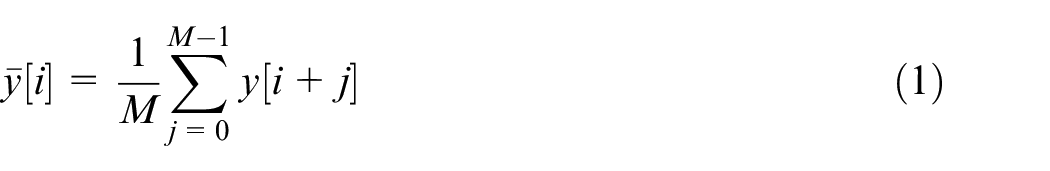
where
In practice, a defined number of samples at a specified sample rate is required to set up this filter. Moreover, all the samples are equally weighted in equation (1). As such, a large number of past samples are required to get a satisfactory performance. Using large number of past samples in calculating the filtered signal introduces delay, thereby making the dynamic response slower. The currently specified moving average filter at the test cells uses 30 samples at a sample rate of 10 Hz, which represents a 3 s length of sample signal and this introduces a dynamic lag of potentially 29 samples or 2.9 s.
Kalman filter
The Kalman filter developed by Kalman 14 is widely recognised as an optimal filter in various engineering applications. Interested readers may consult the review paper 15 and the references therein. In terms of its application to the diesel engine, the Kalman filter had been used to estimate the temperature, nitrogen oxide, ammonia coverage ratio, particulate matter distribution and pressure drop across a diesel catalysed particulate filter etc.16–19 In this study, the Kalman filter is applied to reduce the erratic behaviour of the raw measurements of the backpressure signal and the algorithm as used in Ruppert et al. 20 has been adapted for use in test cells.
The Kalman filter is a cyclic series of calculations run in order to produce an estimate of a process when the true state is unknown. This filter can be tuned to compensate for the process and measurement uncertainty errors in the system. In order to apply Kalman filter, state-space model of the measured back-pressure signal
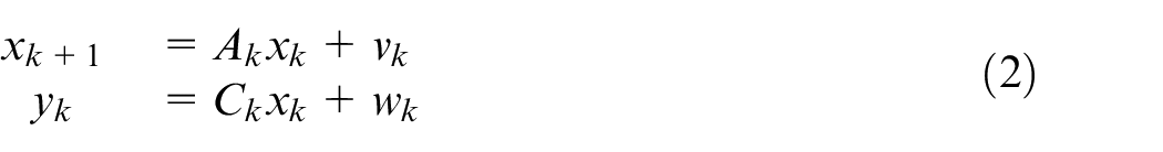
where
The Kalman filter uses a two-stage prediction and correction algorithm, where the prediction stage is given by 21
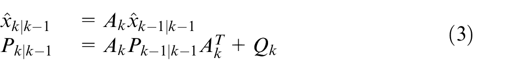
and the correction stage is given by 21
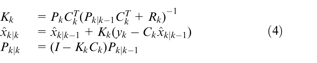
where the subscript
Test cell description
To evaluate the performance of a new engine or to validate a currently existing engine, several tests need to be run on these engines. To run an engine safely, a number of dynamic input and output processes are required as shown in Figure 1. To deliver each of these process inputs to the engine at the specified operating conditions and to recover/recycle the waste outputs, several dedicated process loops for each system are required.
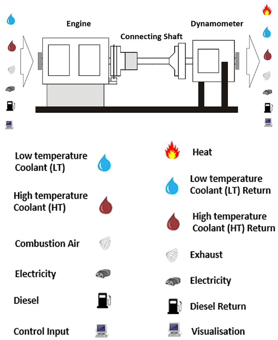
Schematic representation of a test cell process flow with a list of dynamic inputs and outputs processes.
Coolant is required to prevent the engine from overheating. Depending on the engine type, this could be a single loop or split into multiple circuits such as a High Temperature (HT) for piston liner and oil cooling and Low Temperature (LT) for ancillaries such as cylinder heads and turbos. These cooling loops are returned to the cell and maintained at the desired temperature through the use of heat ex-changers through which the engine loop passes. The temperature is maintained by controlling the flow of coolant from the site cooling loop.
To allow the engine combustion to occur requires a supply of clean air. The air is delivered through a series of intake ducts fed from intakes on the plant roof and the restriction is controlled by the use of butterfly valves with electronic actuators.
The engine requires a power supply to operate each of the Engine Control Module (ECM), thus a 27 V power supply and a separate 27 V switched circuit are required. Power is also required for the test cell control system to operate. This is fed directly from the substation and distributed through the Programmable Logic Controller (PLC) hardware, which is used as the controller. This will supply power to the test cell ventilation fans, 24 V starter panel and all the cell Input/Output and data acquisition system.
Another key element for combustion to occur is fuel, which in this case is the diesel fuel. The requirement of the fuel system is to reduce the pressure of the fuel from the main supply, control the temperature as specified by the test and measure the rate of fuel used. This supply is delivered to a gravity fed feeder tank from which the engine can obtain the fuel using the fuel pump.
To evaluate an engine properly, the engine must be able to operate at full running conditions up to and including the ‘rated power’ and ‘torque peak’. This can only be achieved by running the engine against a load, which must be controlled. At these test cells being studied, this is provided by water brake dynamometers. These systems operate by using a series of rotors and stators, which restrict the flow of water through the device producing torque against the engine. As the flow is increased so does the load. The dynamometers require a water supply feed from the central plant supply and return back. To improve the stability of the feed, the water supply is fed to a header tank on the roof of the test facility, which maintains fill control at a set level to provide a consistent head of pressure that dampens out fluctuations in the plant water supply. Both the dynamometer control systems use defined control loops managed by the dyno controllers which regulate the flow of water through the dynamometer by controlling the flow through an output valve. Both systems also have an input valve that can be used to further fine tune the control of the flow.
The final input requirement for the test cell is a central control system and operator interface. The test cell services at the test facility are controlled by a central PLC. This system manages the power supply, processes requests and controls the operation of the cell required to run the engine safely.
These test cells use two types of operating systems for the user interface and data acquisition. They are a central Linux node with the Scientific Linux based CyFlex® and AVL®Puma 2®. These systems provide the user interface to operate and control the engine as well as providing the central data acquisition system for all of the instrumentation. Both systems have configurable software control loops. The software has an in-build option for setting up moving average filters whereas there is no option or function to implement a Kalman Filter. Moreover, there is no way to write the Kalman Filter algorithm into the software in a straight forward manner, and thus some modifications need to be made to facilitate the implementation, which is one of the contributions of this paper. As the setup requirements for implementing Kalman filter are different for each operating system, following two implementations will be described separately.
Implementation of Kalman filter in CyFlex®
Implementing the Kalman filter in CyFlex® is challenging. The calculations can be implemented within the General Labels file but the difficulty comes with implementing the equations for previous Kalman and covariance estimates. These calculations require the capture of the last iteration of the Kalman and covariance estimates. While this is simple to achieve in a cyclic script that most systems use, but the General Labels file in CyFlex does not operate this way. It updates each channel individually on a frequency basis instead. These are updated as described in the file for each parameter, and the frequencies are 1 Hz for SLO, 10 Hz for MED and 50 Hz for FAS. These frequencies are respectively intended as slow, medium and fast sample rates and they are as specified in the system start-up file known as the ‘go’ script for each CyFlex® node. The sample rates are of critical importance as sample rates that are too slow will delay the response and miss the updates. On the other hand, sample rates that are too fast can make the system erratic.
To get around the previous sample problem, a second ‘Running Averages’ specifications file is required. Within this file it is possible to specify an average of a specified number of samples at a specified frequency. From this calculation a number of statistical values can be obtained depending on the suffix. For the Kalman filter implementation, a one-sample running average is required. The file entries for this running at a medium sample rate is shown in Figure 2. By assigning the suffix .FV to the statistical variable, this captures the final value from this data set, which is the previous estimate.
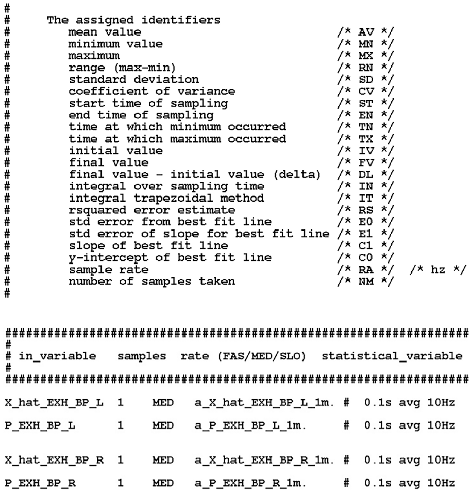
Running averages specifications file in CyFlex®.
The remaining calculations for the Kalman filter are specified in the CyFlex® General Labels file as shown in Figure 3
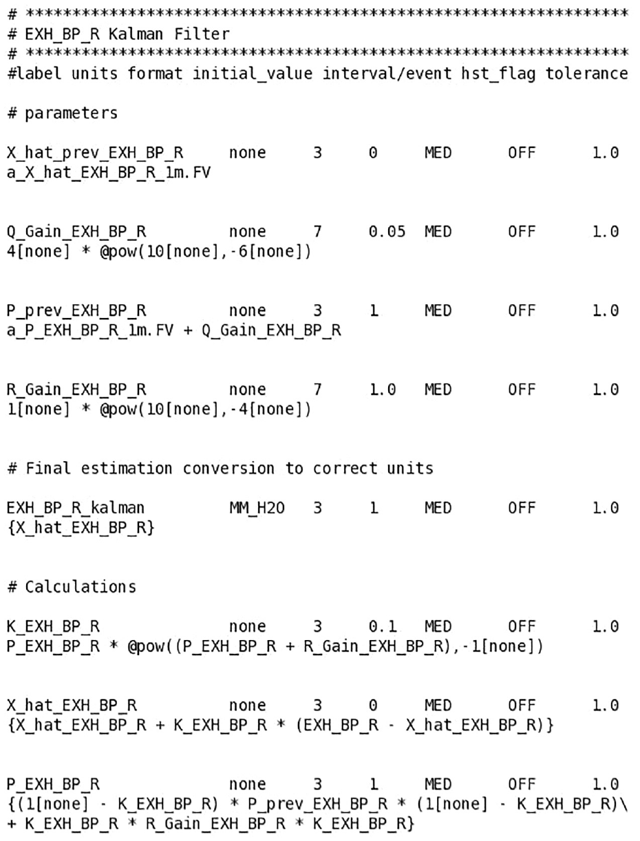
Kalman filter implementation in CyFlex®.
The implementation of the Kalman filter begins with the estimation using the specified parameters
Then, the Kalman filter continues with the calculation of the cyclic variables:
This is then followed by the calculation of the following items:
Finally, the output is obtained and converted back to the unit of
Implementation of Kalman filter in AVL PUMA 2®
To create formulas in AVL PUMA 2®, an input and an output ‘Quantity’ are required. In the case of the output, these are given by the variables ‘EXH_BP_L_Kalman’ and ‘EXH_BP_R_Kalman’. These quantities declare the parameter names, units, decimal places and data types. An example is shown in Figure 4.
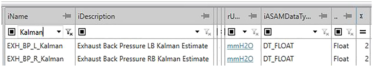
Kalman filter quantities in AVL Puma 2®.
The implementation of the Kalman filter within PUMA AVL 2® is far simpler than in CyFlex® as the Formula Device (FDV) block script can be set to operate cyclically. Therefore, the equations for the previous Kalman and covariance estimates can be updated simply by defining the previous estimates as the estimate from the last iteration of the cycle at the end of the script. There is also no issue with unit conversions, so the use of
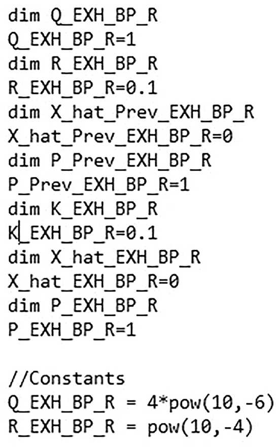
Kalman filter initialisation in Puma AVL 2®.
Each of the calculations is declared as local variables using the ‘dim’ command and the initial values are set using the same values as done in CyFlex®. The covariance parameters
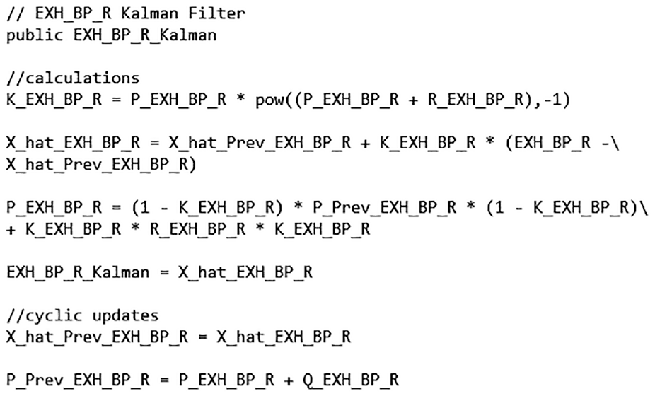
Kalman filter implementation in Puma AVL 2®.
The output is declared as a public variable at the start of the script followed by the cyclic updates for the previous estimates
Results and discussions
Off-line experiment using real data
To obtain accurate prediction or filtering, the covariance parameters of the Kalman filter,
Kalman filter initial tuning value of
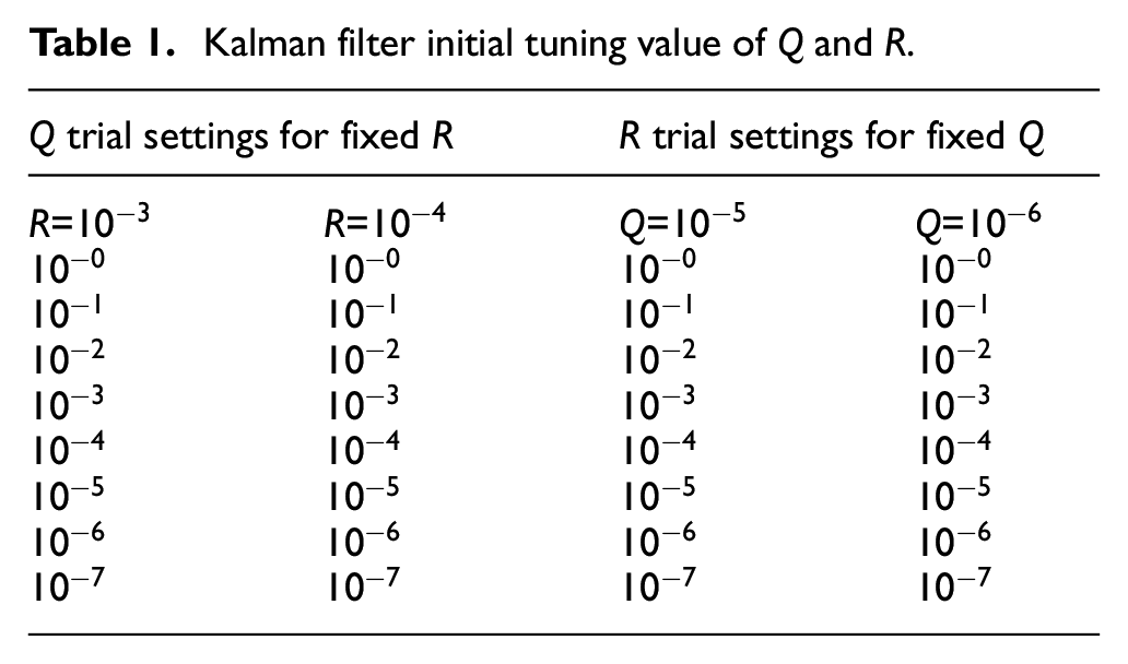
By plotting the various covariance value combinations allows for comparison to determine suitable baseline covariance values. By visual inspection and a prior knowledge of the plant dynamic it is clear from comparing these plots to a fixed criteria that some of the gains are too low resulting in a smooth signal far from the actual. In the cases of too high a gain, the resultant output is close to the original noisy signal. By elimination of the unusable results, this leaves us with the only suitable process covariance
Originally, only the data where the engine is in a steady state condition at rated was compared within the simulation results but it quickly became clear that this single criterion did not give sufficient distinction between the plots to determine the best covariance values as the lack of distinction made it too difficult to shortlist the changes to the covariance gain values. As the filter is intended to improve the dynamic response, it was decided to produce a new simulation script again from passively collected live running data based on a mix of transient and steady state running conditions to allow for the comparison based on both criteria.
From the test cell, suitable range of transient logger data were collected from a cycle test and converted into a simulation script in the same way as for the steady state data. The simulation was repeated using various covariance values as shown in Table 2. Each set of the covariance values was run in turn and the plots were analysed to determine the transient performance compared to the moving average. Those that were closer to the raw value at transient portions were shortlisted for further comparison. The shortlisted gains were highlighted in grey.
Kalman filter final tuning table.
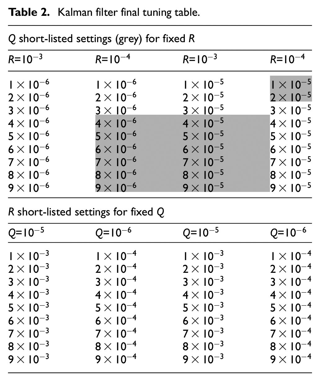
To narrow down the shortlisted selections from the transient tests requires further study of the filter steady state response. From running the steady state simulation for the shortlisted settings, we were able to identify the suitable covariance values. At the higher
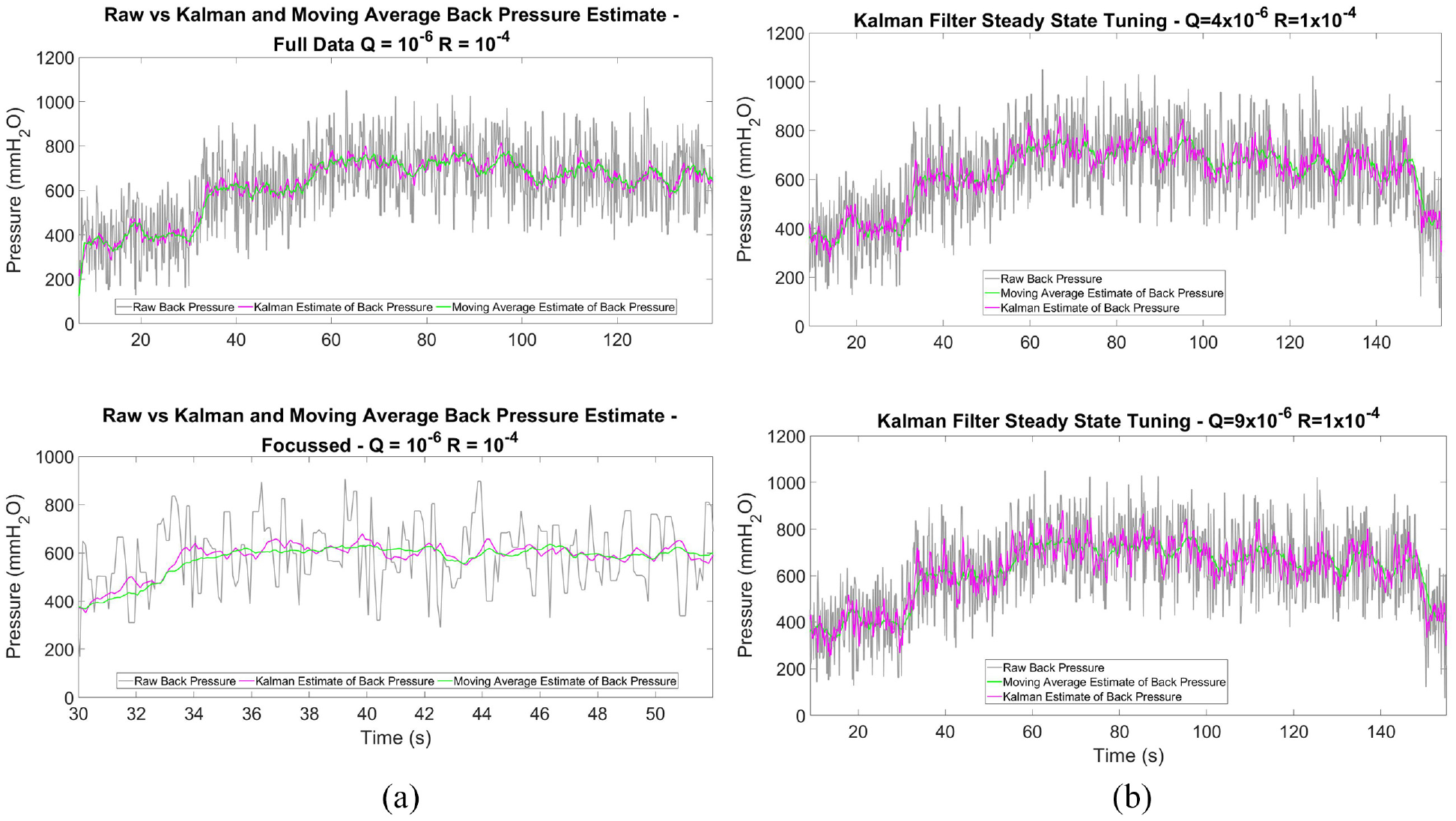
Kalman filter: Steady state tuning comparison. (a) Top: Estimated back-pressure using moving average and Kalman filter with different values of
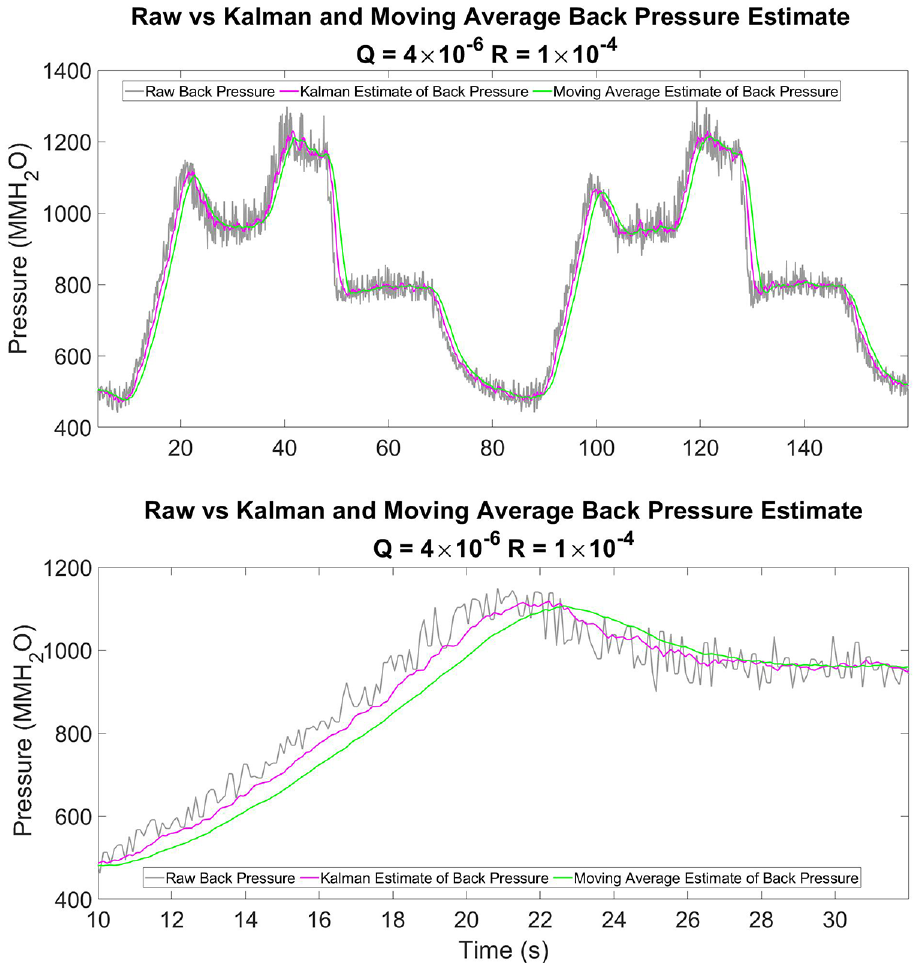
Top: Transient response for moving average and Kalman filters. Bottom: Zoomed-in version between time 10–32 s.
Experimental study
The use of the captured experimental data to produce an off-line simulation script is invaluable for the trial and development of the filter gains, but the final validation can only be achieved by capturing live data from a running engine at the test cell. Here, we make use of the same loggers as the trial script but we change the logger trigger from a ‘start and stop’ command to run automatically when the engine is running. By doing this, it is possible to capture engine data passively during a test. The data used in this case was collected during a cycle test then trimmed to a single cycle which includes transient and steady state engine running conditions such that it can be used for the analysis of the transient and steady state responses of the filter. The results with CyFlex® are shown in Figure 9.
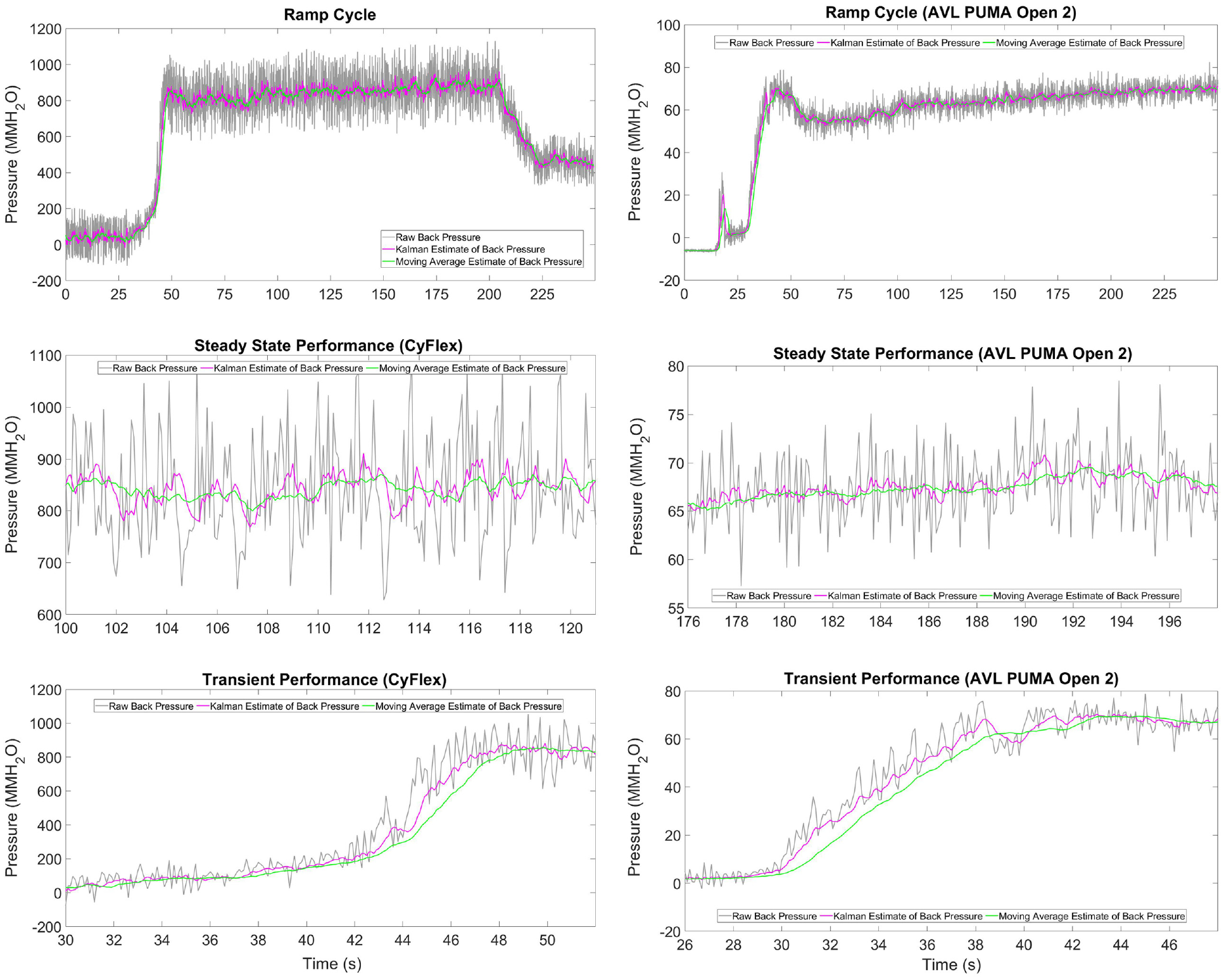
Moving average and Kalman filters applied in CyFlex® (left column) and AVL PUMA 2 ® (right column). Data set shown on the middle and bottom rows are zoomed-in version of the data that focus on steady state and transient responses, respectively. The ramp cycle refers to the build-up behaviour of the back-pressure starting from idle condition (i.e. zero pressure). The steady state performance refers to the stabilise behaviour of the back-pressure after the ramp up stage. The transient performance refers to the duration where the back-pressure ramp up prior stabilising.
These results show the responses of the moving average and Kalman filters as compared to the raw signal. Using the Kalman filter the covariance values can be tuned in accordance with the needs of the application. In this case, the criterion was taken to be a faster transient response in respect of the original signal when compared to the tuned moving average filter but including the most effective filtering at steady state condition. Using this criterion, by comparing the plots it is possible to shortlist suitable covariance values that best meet the criteria. From these plots it can be seen that the Kalman filter tracks the raw signal much closer than the moving average filter throughout the cycle during the transient conditions. However there is a slight trade off in filtering compared to the moving average filter.
For AVL PUMA 2® there is also a recording capability and this requires the set-up of a 10 Hz logger to run automatically. This time the data came from an engine warm-up condition but still shows the transient and steady state behaviours. The results are shown in Figure 9.
This shows sample data collected live from the two types of test cell with the flaps set to the correct operating position manually. The full data set for each is live running data which contains engine transient and steady state rated running conditions to allow for validation of the Kalman filter performance. Again we can see that the Kalman filter outperforms the moving average filter with the results very similar to the one obtained in CyFlex®, thereby verifying the correct implementation in the PUMA AVL 2® environment.
Practical application
To test the effectiveness of the Kalman filter would require its application in a closed loop operation, and its performance is compared with the moving average filter as well as the raw input channel signal. This was tested with a 60 L engine running at the rated speed and load with the control loop reference variable changes between each test. In each case, the controller was started from 100% Open-Loop (valve fully open) and then switched to Closed-Loop to a target of 680
Initially, the raw channel signal was set as the reference signal. For this attempt as shown in Figure 10, the controller was unstable resulting in large controller inputs, which risked damaging the hardware if this was allowed to continue. It was manually set to the expected target but an engine limit was triggered before it could stabilise for long causing the engine to shut down.
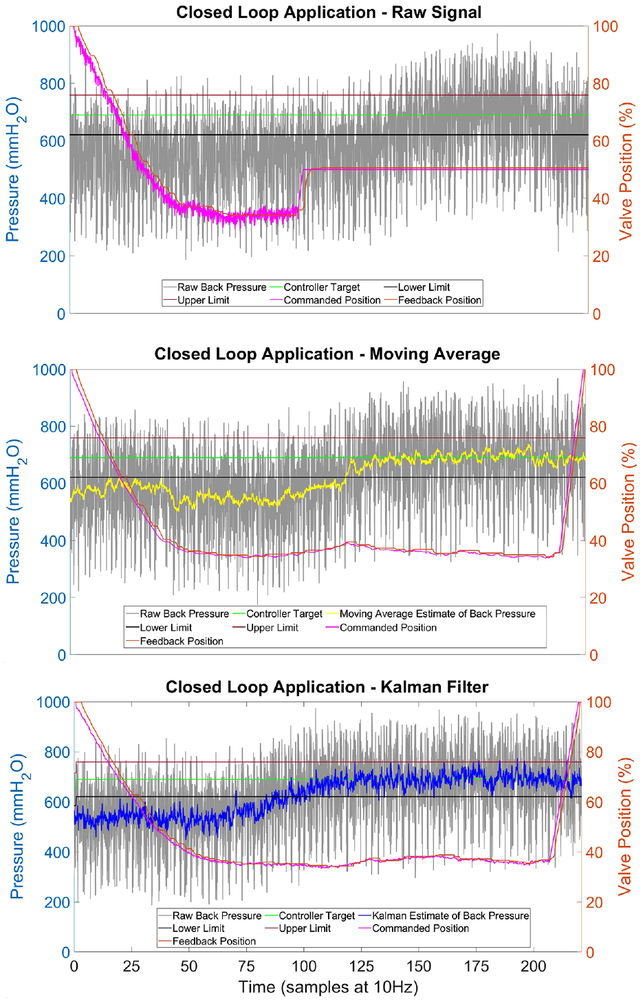
Closed loop control applied in CyFlex® with Raw input (top), moving average (middle) and Kalman filter (bottom) used as reference.
By applying the moving average filter as the reference signal, the control output is more stable as shown in Figure 10. The control output has a smoother response, and it achieved the set-point and reaches steady-state after 150 s.
Finally, we consider the case where the Kalman filter is used as the reference and a similar smooth response can be seen as shown in Figure 10. However, with this reference, the controller reaches the set-point and reaches steady-state after 110 s.
Comparing the three scenarios, we note the following. Without filter, where the raw signal is used as the reference, the erratic behaviour of the signal results in a large controller energy and unstable control. With the application of filters and using the filtered signal as the reference, we can see the improvement. While both the moving average filter and Kalman filter reduce the effect of noise, the Kalman filter has the advantage of having a faster response. In this case 40 s. For an engine which consumes between 3–600 L of diesel at rated condition this time saving would equate to a 3.34–6.67 L of fuel saving for this time duration. As the back-pressure must be set before every test at every cell this can add up to a significant saving in time, fuel, money and emissions output. Nevertheless, both methods require some additional compensation to overcome the resolution of the valve dead-band that prevents the actuator from stabilising.
Conclusion and future works
The common methods for estimating noisy signals in test cells are in the form of simple low pass or moving average filters. Whilst effective, these filters are not necessarily optimal, and in the case of the moving average filter, it introduces lag to the estimate of the dynamical systems.
The Kalman filter, which is an optimal estimator subject to optimal tuning of process and measurement noise covariance matrices, allows for tuning of the algorithm to compensate for measurement uncertainty as well as the process error. Through the careful tuning of the covariance values, the resultant estimate outperforms the moving average filter greatly by reducing the lag seen on a transient cycle and is more responsive at steady state when applied to an exhaust back-pressure signal.
Based on the results obtained in this study, the Kalman Filter shows good potential for improving the back-pressure control of a diesel engine in the CyFlex® environment. The next step will be to test the ability of the existing CyFlex closed loop Proportional-Integral (PI) controller to stabilise to a target and to develop a statistical measurement process to compensate for the low valve resolution and centre to target. Moving forward, the recommendation is to preferably apply the system within the
Footnotes
Acknowledgements
The authors thank Cummins Engine Co. Ltd. for their sponsorship of this project.
Declaration of conflicting interests
The author(s) declared no potential conflicts of interest with respect to the research, authorship, and/or publication of this article.
Funding
The author(s) disclosed receipt of the following financial support for the research, authorship, and/or publication of this article: The work of H. Ahmed is funded through the Sêr Cymru II 80761-BU-103 project by Welsh European Funding Office (WEFO) under the European Regional Development Fund (ERDF).