
Abstract
This study assesses the predictive capability of the ZGB (Zwart-Gerber-Belamri) cavitation model with the RANS (Reynolds Averaged Navier-Stokes), the realizable k-epsilon turbulence model, and compressibility of gas/liquid models for cavitation simulation in a multi-hole fuel injector at different cavitation numbers (CN) for diesel and biodiesel fuels. The prediction results were assessed quantitatively by comparison of predicted velocity profiles with those of measured LDV (Laser Doppler Velocimetry) data. Subsequently, predictions were assessed qualitatively by visual comparison of the predicted void fraction with experimental CCD (Charged Couple Device) recorded images. Both comparisons showed that the model could predict fluid behavior in such a condition with a high level of confidence. Additionally, flow field analysis of numerical results showed the formation of vortices in the injector sac volume. The analysis showed two main types of vortex structures formed. The first kind appeared connecting two adjacent holes and is known as “hole-to-hole” connecting vortices. The second type structure appeared as double “counter-rotating” vortices emerging from the needle wall and entering the injector hole facing it. The use of RANS proved to save significant computational cost and time in predicting the cavitating flow with good accuracy.
Keywords
Introduction
“Direct-injection” technology has significantly improved fuel efficiency, power, and reduced emissions. 1 It uses multi-hole fuel injectors, which operate at very high-pressure over very-short time durations, allowing the precise amount of fuel injected into the engine combustion chamber. However, injecting fuel at very high pressures in such a short duration of time would lead to massive liquid fuel acceleration as it travels within the injector nozzle resulting in the formation of localized low-pressure regions. When the local pressure becomes lower than its saturated vapor pressure, then the liquid starts to boil and form vapor pockets/bubbles; this process is called cavitation. 2
Cavitation in fuel injectors hugely impacts the emerging spray, its stability, fuel breakup/atomization, combustion, and henceforth engine performance. Thus, it has generated a tremendous amount of interest in the research communities, fuel injection system manufacturers, and related industries. Previous experimental studies have identified two primary forms of cavitation structures in these nozzles. The first type is geometrically induced cavitation which initiates at the upper part of the sharp entrance of the injector hole due to the abrupt turn in the fluid path over there and forms a large recirculation zone that extends toward the lower part of the nozzle and forms a horseshoe type recirculation. In turn, it causes a drastic reduction in the cross-sectional area of the nozzle where the passing fuel is forced to accelerate and therefore causing further reduction of pressure and initiation of geometrical cavitation. Besides, when the pressure in the core of the recirculation zones falls below the vapor pressure of the liquid, the liquid starts to form vapor bubbles, following which the cavitation structure convects to the nozzle exit with the fluid.3–10
The quantitative data obtained of the velocity field using the LDV (Laser Doppler Velocimetry) measurements confirm the recirculation region at the upper part of the entrance of the injector hole where geometrically induced cavitation initiates.4,8 However, experimental studies have also shown that cavitation inception occurs at the lower part of the entry of the injector hole when the flow is constricted due to the lower position of the needle9,11 and also its eccentricity. 5 The second type of cavitation structure observed in multi-hole injectors is vortex cavitation which, as mentioned before, originates in vortices when the local pressure in those vortices goes below the liquid-vapor pressure. 6 There are two main types of vortical cavitation observed in several experimental studies. The first type is “hole to hole” connecting vortex cavitation, which has been observed as an arc-shaped vortex, connecting two adjacent holes and the recess between the needle and injector wall.3–5,7,8 The second type of vortex cavitation observed is a twin “counter-rotating” vortical cavitation structure originating from the needle wall and entering the injector hole facing it.7,8,10 All the above-mentioned cavitation structures are believed to be due to the geometry of the injector sac volume and the arrangement of the nozzle holes.
Studies have shown that cavitation directly affects emerging sprays. Cavitation enhances the primary break-up and subsequently atomization of the liquid due to the perceived enhancement of turbulence caused by cavitation. This phenomenon is believed to enhance fuel-air mixing.3,9,11 Experimental studies also indicate that the occurrence of cavitation in fuel injector nozzles led to an enhancement of spray cone angle which also improves the fuel-air mixing as it increases the interfacial fuel area.3,12 However, the cavitation phenomenon disrupts the spray and makes it unstable. Experimental studies have shown that when geometrically induced cavitation originating at the injector hole entrance reaches the nozzle exit, the air from the downstream having higher local pressure than the fuel vapor pressure enters the injector hole. This air entrainment can then replace the cavitation vapor leads to the formation of PHP (partial hydraulic flip) that further enhances spray instability. Besides, the transient nature of cavitation due to turbulence causes further spray instability which influences the performance of the IC engines. 3 It has also been reported13,14 that, apart from fuel vapor cavitation (nucleated), other gaseous voids can simultaneously occur due to the dissolved (non-condensable) gases. Their cavitating nozzle simulation and X-ray fluorescence measurements showed that the presence of dissolved gas in the fuel can cause a significant influence on the total void fraction.
Additionally, the bubbly cavitating fluid behaves like a compressible fluid and the presence of such dispersed bubbles can influence greatly the surrounding liquid flow feature. The presence of even a small fraction of gas/vapor can considerably reduce the local sonic speed of liquid-gas mixture compared to the sonic speed within its constituents, the sonic speed in the bubbly mixture often goes down to 0.1 m/s 2 . This phenomenon occurs because the mixture phase is easily compressed owing to the compressibility of gas bubbles, however, remains dense due to the dominant mass of liquid. 15 Therefore, the bubbly flows in nozzles frequently become locally supersonic which leads to choking and the development of local shockwaves at low speeds which also impairs the nozzle’s performance. 3 Moreover, the violent collapse of the cavitation bubbles which is also supersonic causes localized shocks 2 which adversely affects the mechanical integrity of fuel injectors through surface erosion16,17 besides it also enhances turbulence which affects performance through spray instabilities.2,10,12
Therefore, along with continuous demand to gain a sound understanding of the internal flows in multi-hole injectors through experimental studies, there is an increasing interest in developing and validating CFD models to predict cavitation accurately. LDV measurements have often been used to validate CFD codes for multi-hole automotive fuel injectors. Arcoumanis et al. 4 were the first to evaluate CFD code for multi-hole fuel injector applications with LDV results. They used their in-house single-phase Eulerian CFD Solver to simulate non-cavitating flow conditions in the multi-hole injectors. The comparisons of mean and RMS velocity showed reasonable agreement with the experimental data while it failed to capture the recirculation region at the upper edge of the nozzle entrance; believed to be due to coarse mesh (50,052) and standard k-epsilon turbulence model. 18 The same research group improved their cavitation model 19 by treating the liquid as the continuous phase in the Eulerian frame and cavitating vapor bubbles as a dispersed phase (with many sub-models) and tracked in the Lagrangian frame; the sub-models were used to incorporate many cavitation features such as bubble formation through nucleation, momentum exchange between the bubbly and the liquid phases, bubble growth and collapse due to non-linear dynamics, turbulent bubble dispersion, and both bubble turbulent/hydrodynamic break-up. They quantitatively and qualitatively assessed their model with LDV measurements and high-speed CCD images, respectively, with satisfactory agreements. They later revised their model by incorporating bubble breakup and coalescence submodels to the dispersed phase model 20 and showed good agreement with experimental data including the predicted void fraction with CT (computerized tomography) measurements. It can be argued that their revised model is the most complete cavitation model, however, models have some shortcomings like the assumption of liquid and vapor phase to be incompressible which inhibits the model to describe density change and compressible flow dynamics of the cavitating flows. The number of submodels increases the computational cost and contains many constants that need fine-tuning per specific simulations which add further complexity and empiricism to the simulation. Papoutsakis et al. 21 also used the LDV results of Roth et al. 8 and simulated the non-cavitating conditions. They compared prediction results obtained after LES (Large Eddy Simulation) and RANS simulations. Both results were comparable and were in good agreement with the experimental data. Their study showed no clear advantage of LES over RANS in a similar mesh.
Sou et al. 22 performed CFD simulations using the in-house Eulerian-Lagrangian cavitation model which employed the Rayleigh-Plesset equation to model bubble dynamics. They employed the LES method to simulate turbulence. They validated their prediction results with their captured still images, high-speed video, and LDV measured velocity in a rectangular nozzle. The comparison of prediction results showed good agreements with the experimental results for mean velocity but underpredicted the RMS velocity where cell size was not very fine. The variation in internal flow characteristics and spray patterns in diesel engine from the upper and the lower layer nozzle holes have been investigated recently by Wang et al. 23 experimentally (using X-ray scans) and computationally (using Eulerian-Eulerian two-phase flow and Lagrangian spray models); the results showed that the cavitation development within the upper layer holes is more intense than those formed within the lower layer nozzle holes leading to higher injection rates from the lower layer nozzle holes and that they also exhibit less cycle-to-cycle variations in the observed spray patterns. Also, Mohan et al. 24 simulated in-nozzle flow and spray (flashing and non-flashing) in IC engine using a coupled Eulerian-Lagrangian approach and Lagrangian spray models, and the results showed good quantitative agreements between the liquid and vapor penetration lengths with the published experimental data.
Koukouvinis et al. 25 used the experimental studies of Sou et al. 22 to evaluate their CFD predictions. At first, they attempted using RANS models, followed by the LES simulations. They modeled a cavitation phenomenon using the ZGB turbulence model. Results showed that RANS models failed to capture the cavitation inception adequately, though captured well using the LES method. Also, the comparison between predicted mean and RMS velocity with experimental data showed better agreement than that of Sou et al. 22 prediction, especially on RMS velocity. However, they also mentioned that the computational cost and simulation time of LES is significantly higher than that of RANS. All the above-mentioned studies assumed the vapor phase to be incompressible, which may not represent the true behavior of the cavitation vapor. As was found in the author’s previous studies,26,27 in the cavitating liquid, the vapor formation occurs at the pressure lower than the saturation pressure, where the vapor compression is least likely, however, predicting expansion of the vapor plays a major role in the accuracy of the numerical model.
The present study focuses on developing a sound CFD strategy that will help hydraulic design engineers to design efficient fuel injectors at lower computational cost and within a lesser computational time. The project aims to resolve the cavitating flow in the vertical multi-hole axis-symmetrical diesel fuel injectors having similar geometry to those employed in commercial heavy-duty diesel vehicles. The injector size used in case 8 is a 15X replica of an enlarged Bosch vertical axis-symmetrical fuel injector at the full lift representing the fully open fuel injector position with a reported quasi-steady flow regime. It should be mentioned that the transient effects of the injector (during needle opening and closing) on the internal nozzle flow haven’t been modeled in this study. Although the transient effect is over a short period of time, it has a great impact on internal flow structure, especially at high injection pressures with diesel injectors, which influences the near field emerging spray and then atomization and combustion. The subject has been investigated previously and the most recent experimental work 28 used X-ray imaging and showed the transient behavior of liquid jet at the nozzle exit. Also, Strotos et al. 29 simulated the transient heating effects in high-pressure diesel injector and showed that increasing the injection pressure from 2000 to 3000 bar, caused a considerable increase in fluid temperature to above the boiling point and thus leading to fuel boiling and instability.
In the present study, two flow conditions are simulated with CN = 1.48 and Re = 34,100 and CN = 4.57 and Re = 39,500, under steady flow condition and the flow is wall-bounded Hence, to simulate these flow conditions, the RANS approach appeared to be most appropriate due to its ability to predict such flows efficiently with competent accuracy and with lesser computational cost and time. The authors opted for the realizable k-epsilon model 30 for this study as in the comparative assessment of the author’s previous work, 26 it was observed that the realizable k-epsilon model gave the most accurate prediction for this class (internal flow of multi-hole fuel injectors) of flows. The chosen cavitation model is ZGB 31 that uses the Linear Rayleigh Equation 32 to model bubble growth, and that its collapse is dependent on the pressure differential across the bubble surface. Even though there are similar models based on the Linear Rayleigh equation, recent studies have shown that the ZGB model provided a more accurate prediction than its counterparts.26,27,33 The Eulerian mixture multiphase model34,35 is used with the cavitation model in this study. The Eulerian mixture model approach solves one set of conservation equations for mass, momentum, and energy with a volume fraction transport equation for the second phase with a turbulence closure model, making it computationally more efficient than the other Eulerian Multifluid model. The Eulerian Multifluid 36 model set of mass, momentum, and energy conservation equations for each phase and achieves coupling through pressure and interphase coefficients hence the Eulerian Multifluid model is more complex and computationally more expensive than the mixture model. Both approaches allow phases to be interpenetrating or polydisperse as perceived in cavitating flows. The multifluid model can be argued to be more accurate than the mixture model, however, a previous comparative study 33 did not exhibit a distinct advantage of one approach over the other. Therefore, the mixture model is the approach adopted in the present study. Also, in the present study both liquid and vapor were assumed to be compressible, which to the authors’ knowledge it is for the first time to be done for the considered geometry. However, the compressibility of multiphase flow has been considered in other flow geometry like that by Mithun et al. 37 who have reported a barotropic three-phase model to simulate water injection into the atmosphere and assumed all the phases (water, vapor, and air) to be compressible. As the cavitation phenomenon is perceived to be isothermal, therefore the liquid compressibility is modeled using the Tait equation, 38 which is a well-known EOS (equation of state) and is used to relate liquid density to change in local pressure. It is an isentropic equation, based on experimentally determined parameters. The Tait equation has advantages owing to its ability to handle both high and low-end pressures. 39 The compressibility of the vapor state is modeled using the ideal gas law. The paper will assess the predictions by comparison of predicted mean velocity and RMS velocity with LDV measured data and the predicted cavitation volume with the recorded CCD images.
Flow configuration
Roth et al. 8 performed experiments on a 20x enlarged transparent multi-hole axis-symmetric fuel injector nozzle that represented the geometry of Bosch conical mini-sac type six-hole axisymmetric vertical diesel fuel injector as shown in Figure 1. They measured mean axial velocity and RMS velocity at different axial locations as specified in Figure 2 within the injector hole and high-speed imaging to capture cavitation occurrence and its development inside the fuel injector.
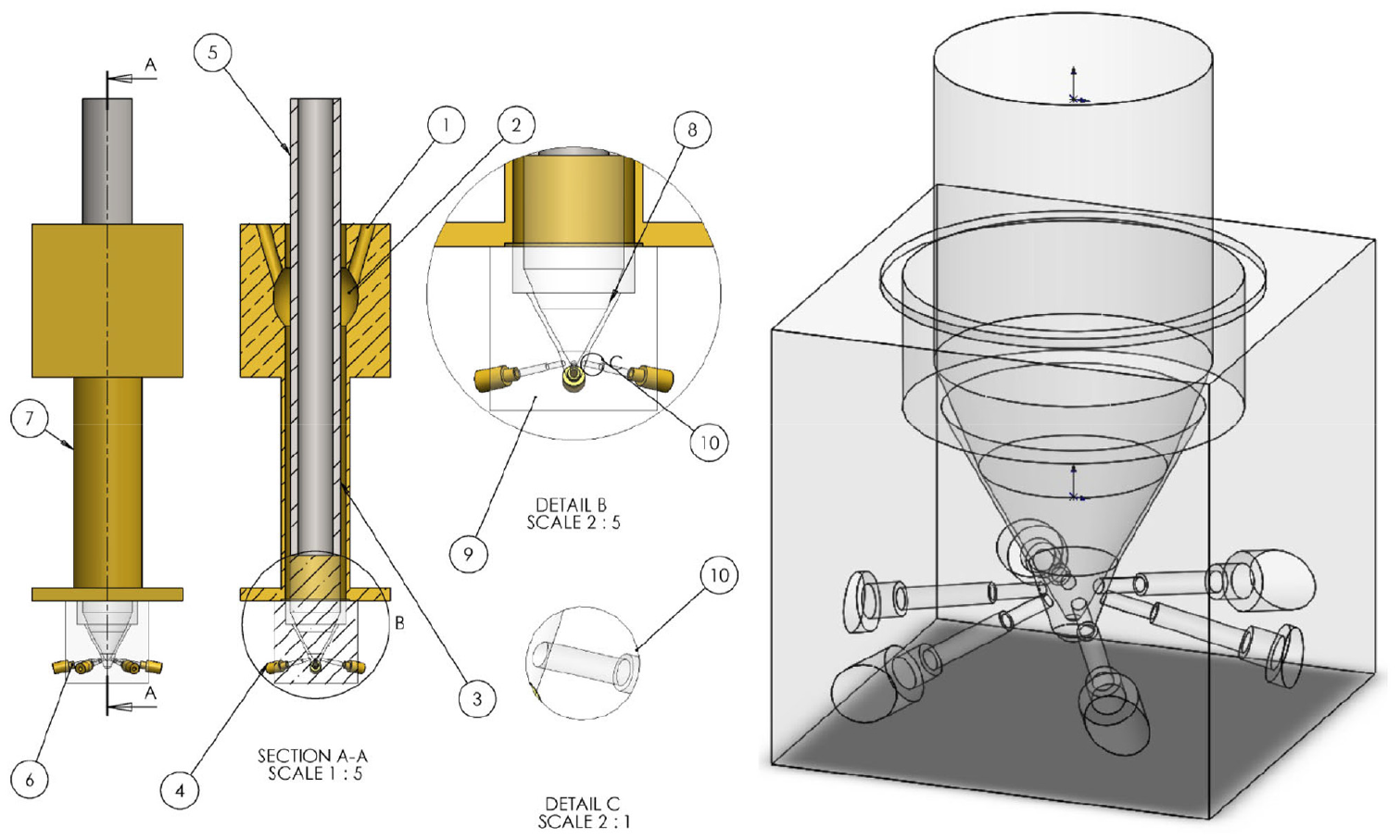
Representation of the refractive index matching test rig with the 3D model of the transparent enlarged conical mini-sac injector as of Roth et al. 8
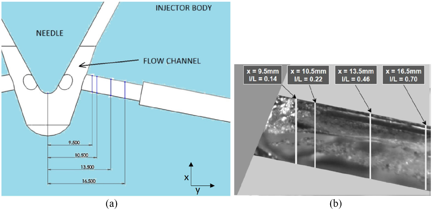
(a) Sketch showing the needle and injector assembly and the positions where the prediction of mean and RMS velocity were made and (b) recorded locations in experimental data. 8
The nozzle was made of acrylic with a refractive index of 1.49. The working fluid was a mixture of 32% by volume of tetralin (1,2,3,4-tetrahydronaphthalene) and 68% by volume of oil of turpentine. The working fluid had a density of 895 kg/m3, the kinematic viscosity of Pa.s with a vapor pressure of 1000 Pa. The mixture was maintained at a temperature of 25 °C± 0.5°C to keep the refractive index of the mixture and the acrylic at 1.49. The refractive index matching technique enabled full optical access to the complex flow geometry, near the wall and liquid-vapor interface with no distortion of the laser beam. 40 The nozzle operated at the fixed needle lifts, the operating conditions used for CFD simulations in the present study are listed in Table 1, the same as those used by Roth et al. 8
Operating conditions.
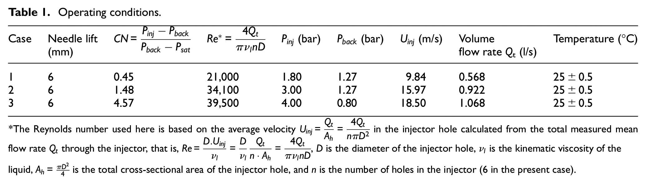
The Reynolds number used here is based on the average velocity
Methodology
Mixture model
The mixture model solves one set of conservation equations for mass, momentum, and energy and the volume fraction transport equation for the second phase with the addition of the turbulence closure model. The model assumes equal velocity, temperature, and pressure between phases. within a minuscule time scale (almost instantly). Hence, the resulting equations resemble this assumption is based on the notion that the difference between three potential variables would facilitate mass, momentum, and energy transfer between phases so fast that equilibrium would be achieved pseudo-fluid with mixture properties and the equation of state which links phases, so mixture thermodynamics properties are obtained.34,35 The model equations are presented in the steady-state form.
The following formulation is used to calculate mixture density:
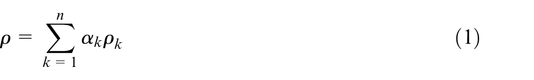
where

Since,

Hence, equation (2) becomes:

Similarly, the viscosity of the mixture can also be calculated as:

where
The continuity and momentum equations are as follows:


where
Cavitation model
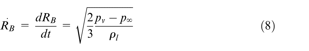
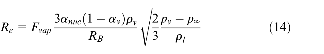
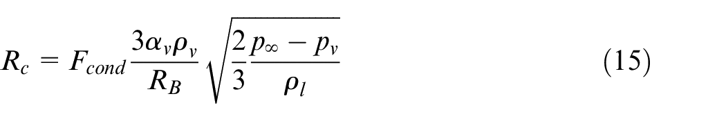
The ZGB model 31 is a rate-based cavitation model and it describes the bubble growth (vapor production during cavitation) and collapse (condensation at higher local pressure) using the Rayleigh relation (equation (8)). The rate term is integrated into the vapor fraction transport equation (equation (10)).
where
The model defines the vapor volume fraction using the following equation:
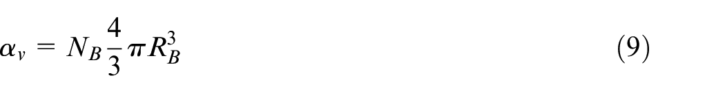
where
The transport equation for the vapor fraction is:

where R is again the net phase change rate and is defined using the following equation:
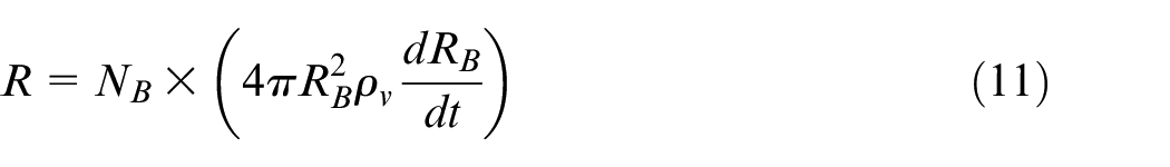
The phase transfer rate terms are as follows:
When

When
Zwart et al.
31
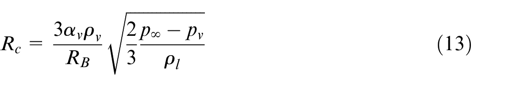
reported that the model works well for condensation but produces physically incorrect results and numerically unstable when employed for cavitation. This is because the model assumes no interaction between the cavitation bubbles, which is only possible in the early stages of cavitation when cavitation bubbles grow from a nucleation site. However, they mentioned that when the vapor volume increases, the nucleation site density must decrease accordingly. Hence, Zwart et al. proposed to replace
When
When
The values of model constants are
Liquid and vapor compressibility models
Tait equation – liquid compressibility model
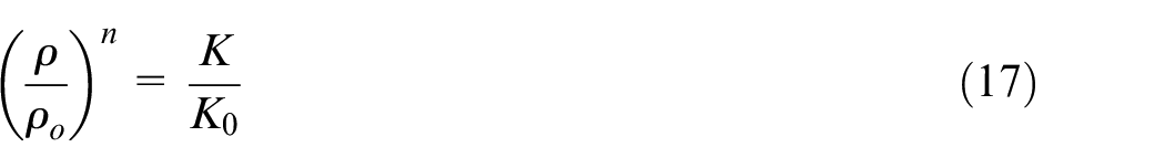
The Tait equation 38 establishes a nonlinear relation between the density of the liquid and its pressure under isothermal conditions. It can be expressed in terms of pressure and density using the following relationship:

where a and b are coefficients that can be defined by assuming that bulk modulus is a linear function of pressure, the values of a and b are based on the reference state values of pressure, density, and bulk modulus. n is known as a density exponent, having a similar role as a ratio of specific heats. 41
The simplified Tait equation as implemented in the ANSYS Fluent platform has the following formula 42 :
where

and

where
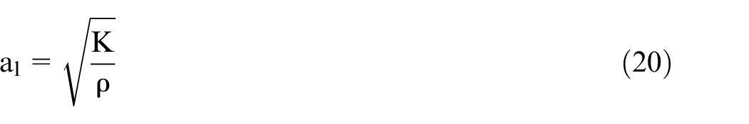
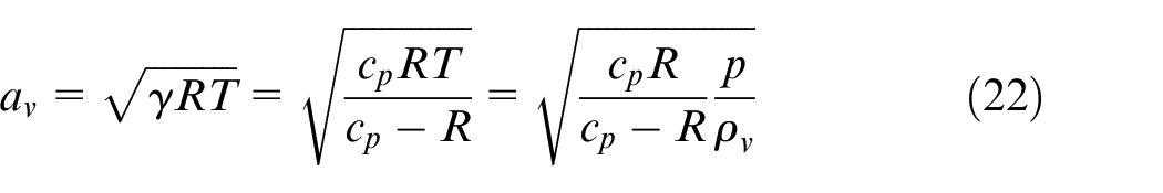
The speed of sound in the liquid phase is calculated using the following equation:
Ideal gas law
The vapor density is modeled using the ideal gas law which has the following form:
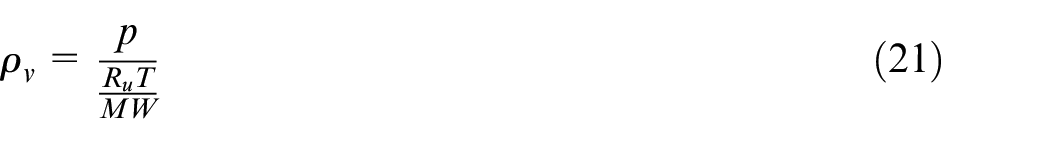
where
where
where R is the specific gas constant
Sonic speed in mixture phase model
The speed of sound in the mixture phase is computed using the Wallis Model, 43 the model assumes local thermodynamic equilibrium between phases and has been implemented in the following form in ANSYS Fluent: 44
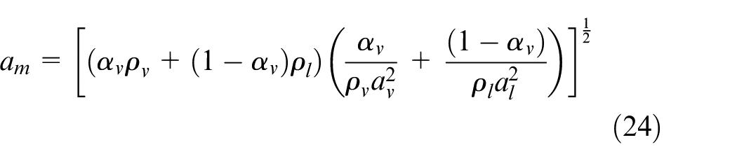
where
Numerical methods
The governing equations are solved using commercial CFD solver ANSYS Fluent v14.5 which uses the Finite Volume Method.
45
Acknowledging that the flow regime is quasi-steady,
8
steady-state simulations are performed. The SIMPLE algorithm
46
was employed for pressure-velocity coupling. The geometry of the nozzle is axis-symmetrical with six holes
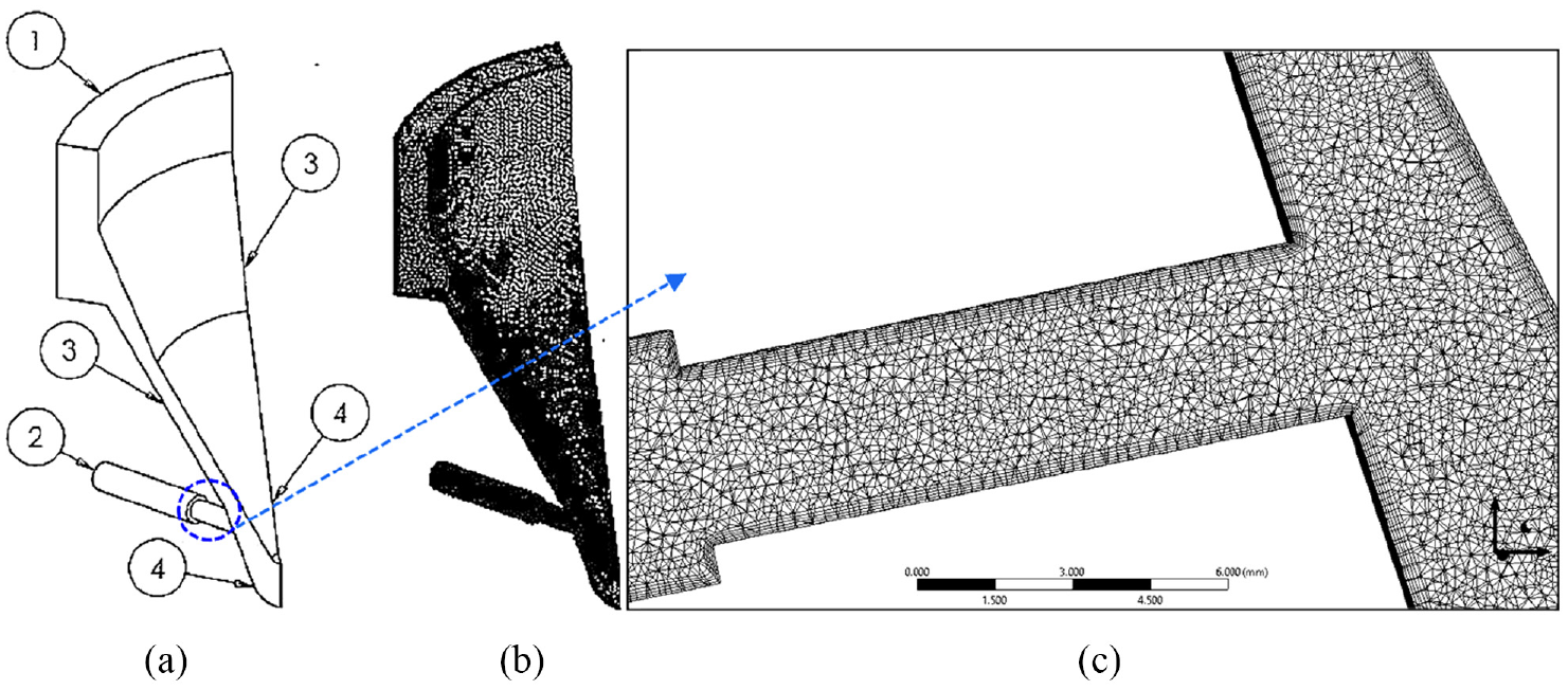
(a) One-sixth of the flow domain at the full needle lift with periodic (cyclic) boundary conditions. The numbers represent the boundaries of flow domains, (1) inlet (2) outlet (3) walls (4) periodic (cyclic) interface, (b) Mesh of the fluid domain, and (c) axial plane mesh of the nozzle flow domain.
Grid used at non-cavitating conditions.
Grid used at cavitating conditions.
Results and discussions
Numerical analysis and comparison with experimental results
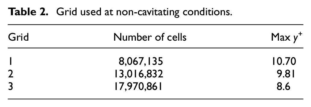
At first, the mesh convergence study was performed at non-cavitation conditions at CN = 0.45 as described in Table 1 using grids 1, 2, and 3 as given in Table 2; noted that since the simulation is under steady-state, it was stopped when residuals reached convergence criteria, 1e − 04. The comparison of predicted mean axial velocity profiles at various axial locations indicate similar predictions obtained using grids 1, 2, and 3 as shown in Figure 4 on the left column. However, grid convergence results for RMS velocity shown in Figures 4 (right column) present different insights. The comparisons show that RMS velocity increases slightly with the increase in mesh density, especially where the mean velocity gradient is the highest. This is because as the grid density increases, the magnitude of mean velocity gradients also increases. The Boussinesq formulation 45 is used in the RANS method to compute the RMS velocity. In this method, the RMS velocity magnitude depends directly on mean velocity gradients. The increment in RMS velocity with an increase in mesh density indicates an increase in mean velocity gradients as the mesh density increases. Overall, the mesh convergence results show satisfactory agreements between grids 1, 2, and 3 therefore, grid 2 is selected for analysis.
Normalized mean axial velocity (left column) component and the corresponding RMS velocity (right column) of non cavitating nozzle flow at CN = 0.45: (a) x = 9.5 mm, (b) x = 10.5 mm, (c) x = 13.5 mm, and (d) x = 9.5 mm from the entrance.
At x = 9.5 and 10.5 mm (Figure 4(a) and (b)) close to nozzle entrance, the comparison of experimental data of series 1 and 2 shows small discrepancies that are said to be due to the possibility of needle eccentricity. 20 Nevertheless, comparisons in Figure 6(a) and (b), right column, show that at the axial position close to the entrance and upper end of the injector hole (0.8<y/D′ < 1), the numerical simulations captured the recirculation region with adequate accuracy. Also, on the same locations in Figure 6(a) and (b) (right column), the predicted RMS velocity results indicate reasonable agreement with the experiment. Further downstream on the plane x = 13.5 mm, the mean velocity predictions indicate good agreement achieved with experimental measurements in Figure 4(c) while the calculated RMS velocity, Figure 4(c), indicates an underprediction, however, it has achieved the same trend as the experimental data. Similarly, on the position x = 16.5 the predicted mean velocity results in Figure 4(d) suggest good agreements with the experimental data and the same results for the RMS velocity as that seen in Figure 4(c).
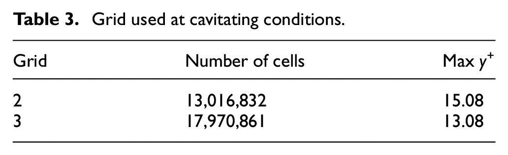
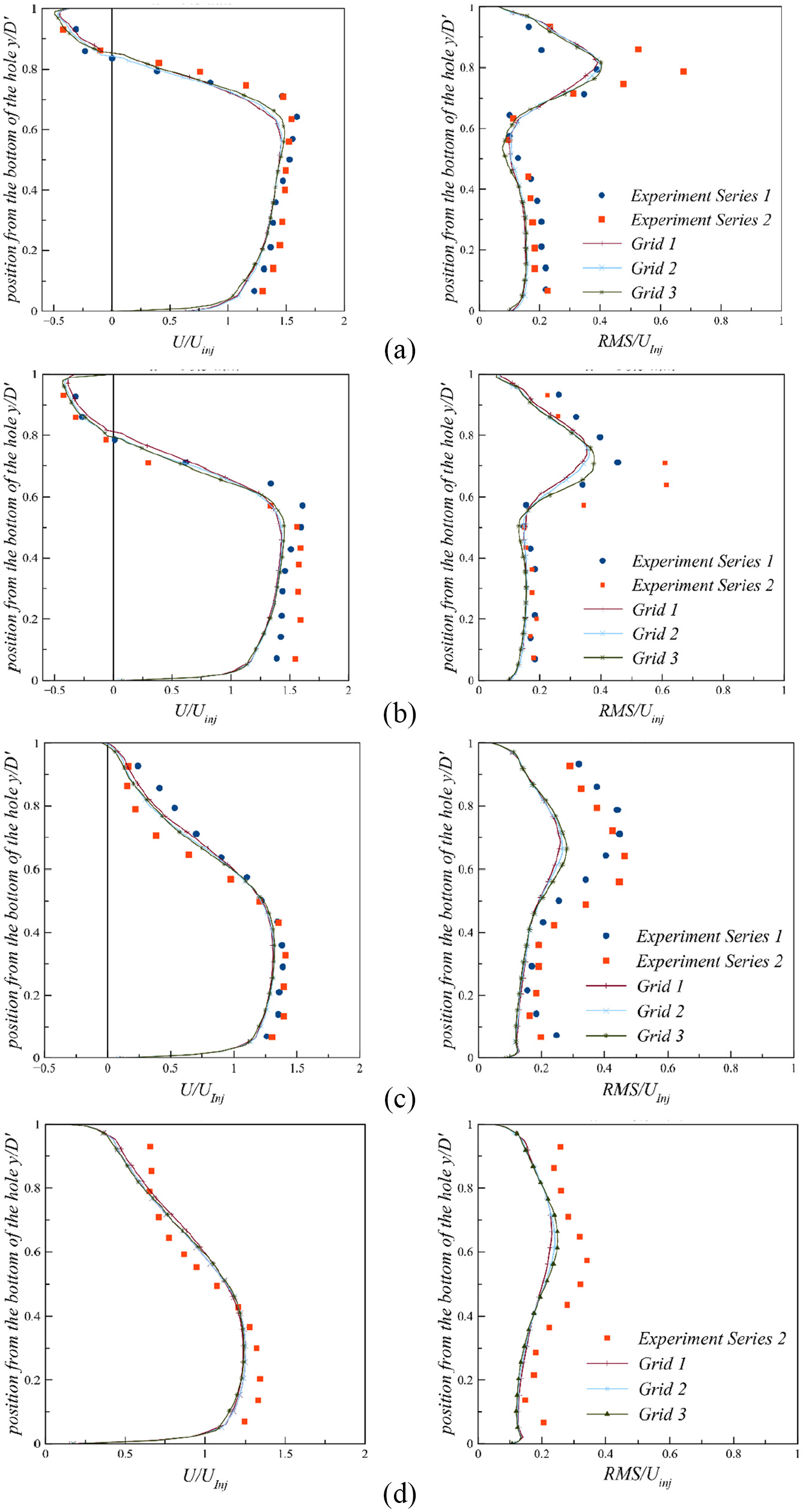
After achieving an overall good agreement at non-cavitating conditions, it was decided to simulate the flow under cavitating conditions CN = 1.48 and 4.57 and the results of the axial mean (left column) and RMS (right column) velocity profiles at different axial locations along the nozzle are shown in Figure 5. Grid independence was again checked at CN = 1.48 that can be seen in Figure 5 for mean and RMS velocity at all x-locations and also in Figure 6 where the distribution of predicted vapor volume fractions at all x-locations are shown. Grid 2 and 3 from the non-cavitating simulations were used, however, it was found unjustified to perform cavitation simulations in all three grids as the first grid is often not selected for analysis in CFD simulations. The grid independence study was performed considering both phases to be incompressible. The predictions suggest similar results achieved for mean velocity using both grids as seen in Figures 5, left column, while the RMS results on the right column indicate a slight increase in the RMS magnitude with an increase in cell density with grid 3, which, as mentioned before, is due to the tiny upsurge in the mean velocity gradients with an increase in the numbers of cells in the grid.
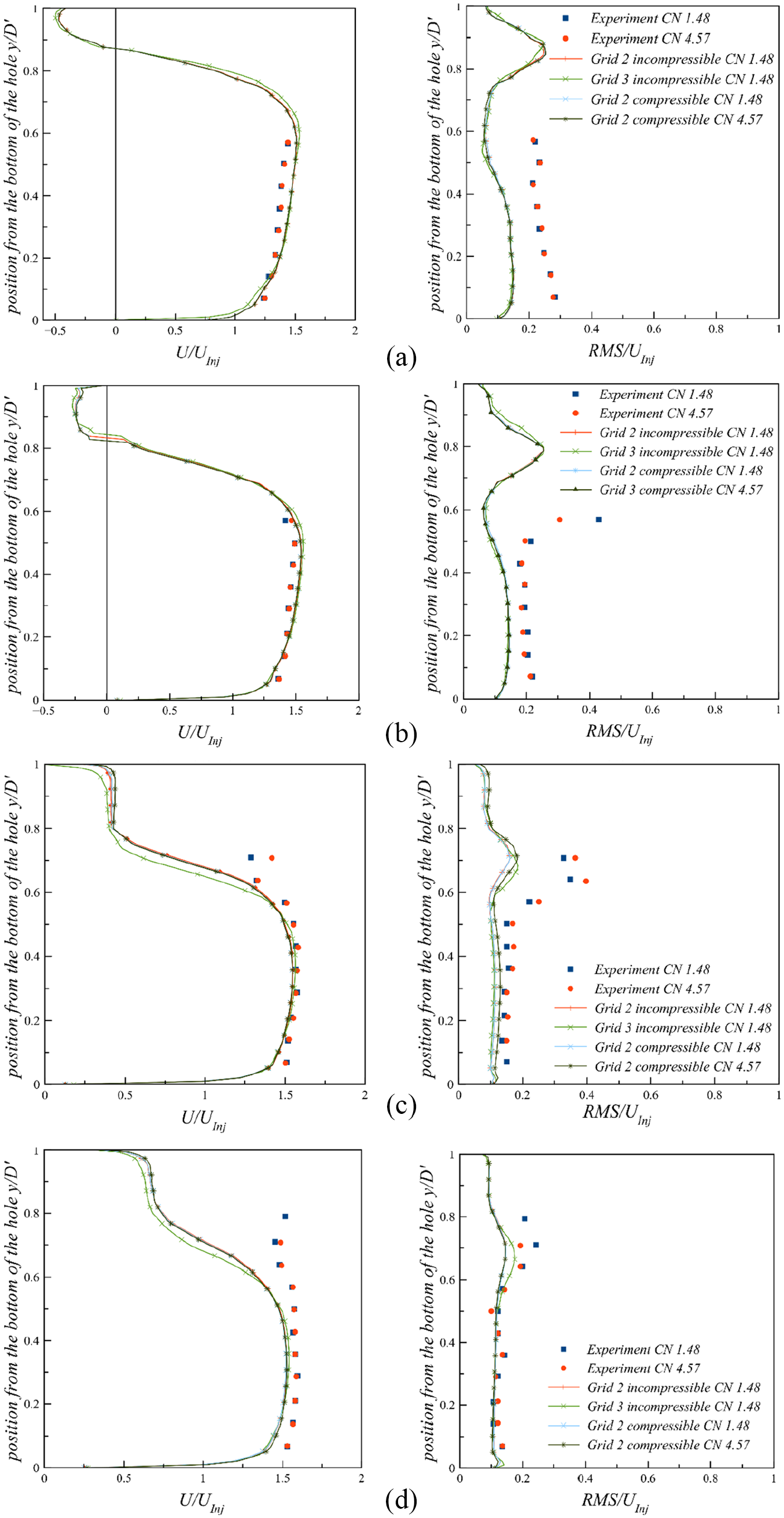
Normalized mean axial velocity (left column) component and the corresponding RMS velocity (right column) of cavitating nozzle flow at CN = 1.48 and CN = 4.57: (a) x = 9.5 mm, (b) x = 10.5 mm, (c) x = 13.5 mm, and (d) x = 9.5 mm from the entrance.
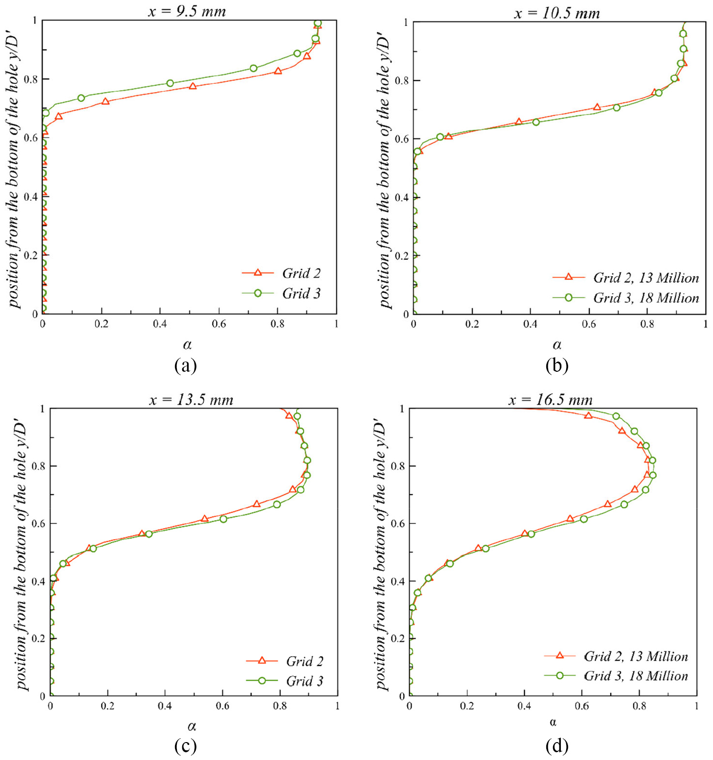
Effect of the number of cells in the grid on distribution of predicted vapor volume fraction, α, across the nozzle at locations x = 9.5, 10.5, 13.5, and 16.5 using grids 2 and 3 at CN = 1.49.
The comparisons for the vapor volume fraction of Figure 6 indicate a slightly higher production of vapor obtained using the mesh with a higher cell density of grid 3 than grid 2. This can be attributed to steeper pressure gradients obtained using a mesh with higher cell density. However, the grid independence study provided satisfactory overall agreements between grids 2 and 3. Hence the grid 2 was selected for further analysis and simulations to make the optimal use of computational resources and time because to simulate incompressible cavitating flow with grid 3, the cluster computer with 16 cores took around 18 days to complete the task and the results did not show any significant advantages. Also, Figure 10 confirms that the cavitation originates at the upper edge of the entrance of the nozzle due to the presence of low-pressure zones where the recirculation region is formed with the highest amount of vapor. The results also show that the vapor spread from the near upper part of the nozzle toward the lower part as the cavitated fluid convects downstream so that at x = 9.5 mm the vapor occupies an area from y/D′ ≈ 0.65 to y/D′ = 1 while at x = 16.5 mm the vapor expands and spreads to an area from y/D′ ≈ 0.25 to y/D′ = 1.
On comparing results of grid 2 at CN = 1.48 at x = 9.5 and 10.5 mm in Figure 5(a) and (b) assuming phases to be incompressible and compressible (using Tait, for liquid, and ideal gas, for vapor, equations), the mean and RMS velocity results are found to be comparable with no appreciable differences; also, the predicted values in mean and RMS of grid 2 at CN = 4.57 were found to be similar to those at CN = 1.48; similar results can be seen at other x-location. These results suggest that the influence of compressibility on mean and RMS velocity, within the calculated CN range, is not evident. However, at higher CN, one would expect to see higher RMS values when assuming phases to be compressible due to the expansion of vapor that causes an increase in its volume, which leads to a decrease in density and hence higher turbulence.
On observing the experimental mean axial velocity and RMS velocity at both CN = 1.48 and 4.57 at all x-positions in Figures 5, it can be seen that experimental values are only available for the bottom of the injector orifice to just above the middle it, that is, 0 < y/D′ < 0.6, due to the presence of dense vapor there that affect the refractive index of the liquid and the laser beam deflection/diffraction, and hence prevented accurate liquid phase LDV measurements, 40 which possibly allowed LDV measurements by Roth et.al. 8 to be made only at positions where vapor was not present. At all x-positions, the comparison of predicted mean velocity with that of experimentally recorded indicates good agreements for both CNs as shown in Figures 5 (left column). The comparison of predicted RMS velocity with experimental data at these positions at both CNs in Figures 5 (right column) also good agreements achieved from the bottom to the middle of the nozzle (0 < y/D′ < 0.5). However, at the upper portion of the nozzle (0.5 < y/D′ < 0.8) since the experimental data is not available, therefore no comments can be made regarding the accuracy of predictions for this section of the injector hole.
In the grid independence study, both phases were assumed to be incompressible. However, in later analysis, the density of both liquid and vapor phases was considered to be compressible that also allows the fluid volume of these phases to be variable. As aforementioned, in the liquid at the local pressure lower than the saturation pressure at which the cavitation initiates, the vapor compression may be insignificant, but its expansion is a dominant phenomenon and needs to be modeled appropriately. At the same time, the vapor expansion is likely to displace and compress the liquid, and therefore, liquid compressibility is also modeled in this case study, although the author’s previous studies have shown that liquid compressibility assumption played an insignificant role in affecting the overall flow field at the range of cavitation numbers of this study. Figure 7 compares the predicted cavitation vapor fraction assuming phases to be incompressible (Figure 7(a)) and compressible (Figure 7(b)) at CN = 1.48. The results show a lower volume of cavitation vapor predicted when assuming the vapor phase to be incompressible than the compressible.
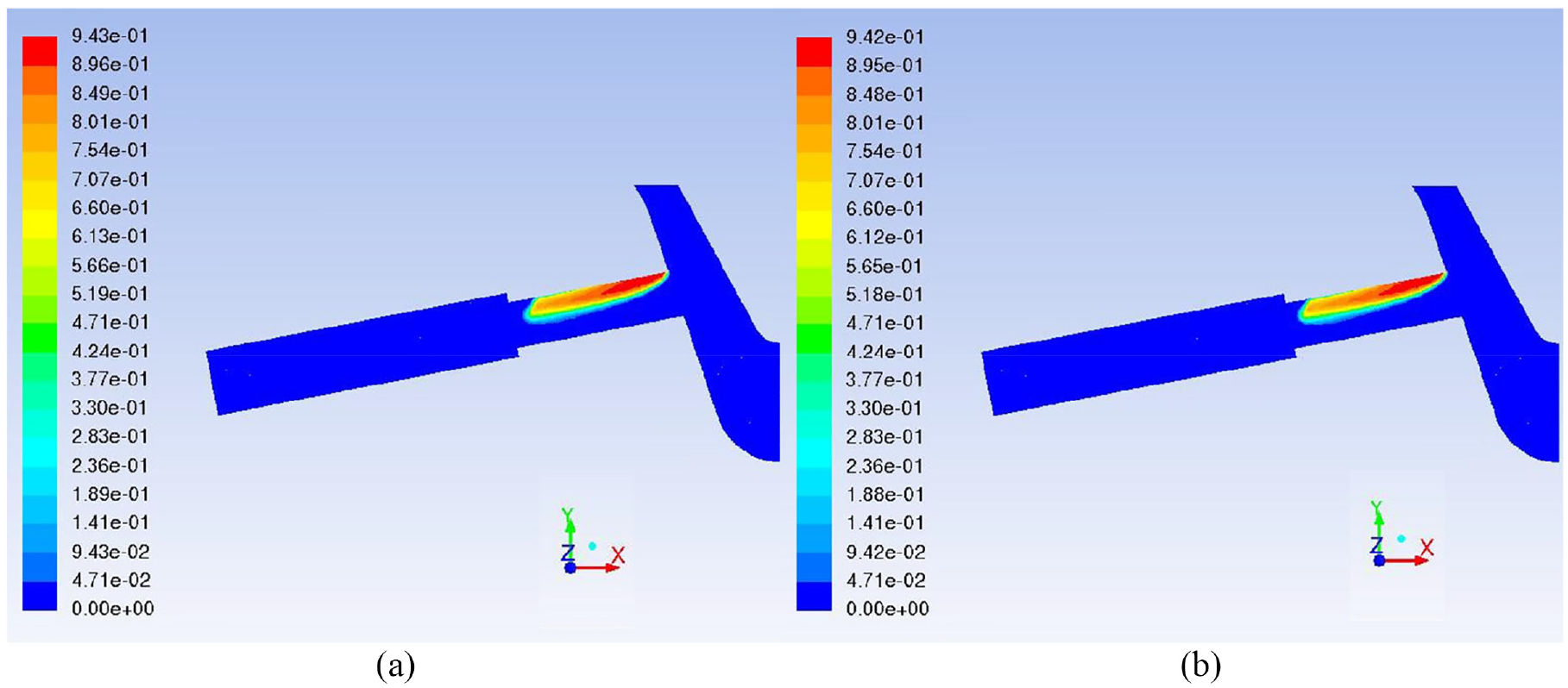
Comparison of predicted vapor fraction at CN = 1.48: (a) incompressible gas and liquid assumption and (b) ideal gas assumption for vapor, and Tait equation for the compressible liquid.
Figures 8 and 9 show the isosurface of vorticity (0.5% of the magnitude) in the x-y plane for CN = 1.48 and 4.57, respectively. 3D isosurface of vorticity has been generated in order to detect the formation of vortical structures; 0.5% of the vorticity magnitude of isosurface was found to provide the best representation of the overall shape of the vortical structures in the nozzle. The results show the presence of a complex flow structure within the sac volume, upstream of the nozzle entrance, inside the nozzle, and within the exit step sudden expansion at both CNs. The key flow features are highlighted on the figures like a hole-to-hole vortex, the origin of the counter-rotating vortices, and its merger with hole-to-hole vortex, the recirculation zone, and its reattachment and cavitation. On observing the cavitation flow field in Figure 8 at CN = 1.48, it can be seen that cavitation originates at the upper edge of the entrance of the nozzle. This, as aforementioned, is due to the formation of low-pressure zones at the recirculation region at the upper portion of the injector hole entrance. The results also show that the cavitation bubbles are convected downstream on the upper part of the hole up to a distance of 87% of the nozzle length where they start to collapse before reaching the exit step sudden expansion. At higher CN of 4.57, Figure 9, similar flow structures to that at lower CN can be seen, but since the cavitation is more intense at higher CN, the cavitating bubbles are convected over the hole length of the nozzle and enter the backflow hole of the step expansion and lead to the development of the annular recirculation region or annular ring-shaped step vortex which also enhances cavitation. The cavitation structure forms a liquid-vapor fluid mixture (cavitation cloud) as it further travels downstream.
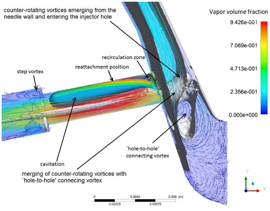
Flow description in the injector at CN = 1.49. The cavitation is shown using 3D isosurfaces of vapor volume fraction together with velocity vectors to describe the flow profile.
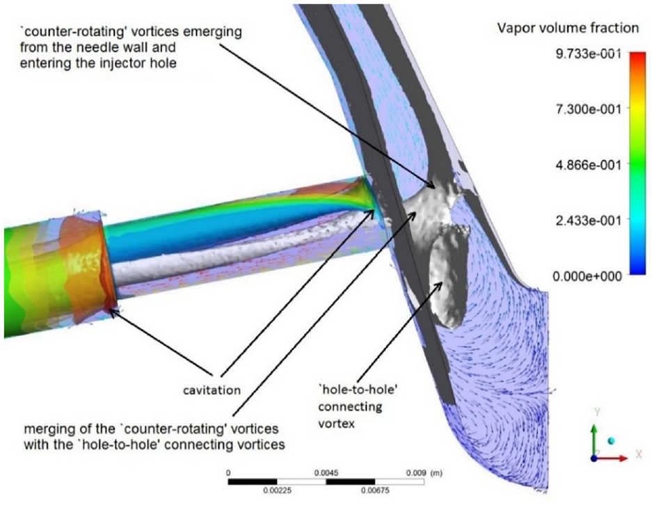
Flow description in the injector at CN = 4.57. The cavitation is shown using 3D isosurfaces of vapor volume fraction together with velocity vectors to describe the flow profile.
To further analyze the flow field, velocity vectors, and isosurface of vorticity of 0.5% vorticity magnitude are presented in Figure 10. The velocity vectors clearly show the prediction of vortical structures mentioned in numerous experimental studies.3–5,7,8,10 The first type of predicted vortical structure is the “hole-to-hole” connecting vortex which is seen connecting two adjacent injector holes in the experimental studies. The other type of vortical structure predicted is twin “counter-rotating” vortices emerging from the needle wall and entering the injector hole facing it. An explanation has been provided in the next paragraph as to how these vortices are formed.
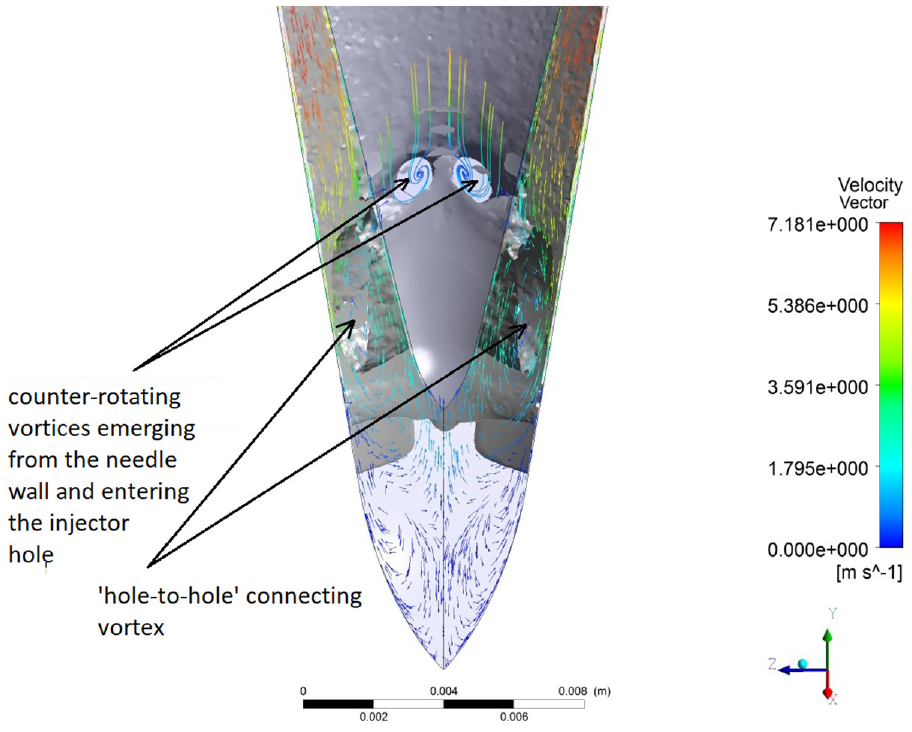
Predicted velocity vectors and streamlines and isosurface of vorticity (0.5% of magnitude) at CN = 4.57 showing “hole-to-hole” connecting vortices and double “counter-rotating” vortices.
These vortices in the multi-hole injectors, in particular, in the present geometry could be due to the peculiar flow pattern owing to its complex geometry. The nozzle’s cavity or the flow volume is shaped like a hollow section of two cones stacked one on another (as can be seen in Figure 2(a)), to accelerate the fluid in symmetrically placed six holes for the fluid exit. As the liquid convects, the lower pressure in the injector holes would attract most of the liquid and accelerate the fluid toward the exit. However, some proportion of the fluid that does not enter the injector holes and due to fluid momentum, it tends to enter the sac volume toward the needle tip. The already present fluid in the sac volume would exert resistance to more fluid entering the limited sac volume and hence would lead to the formation of vortices around the injector hole. The proportion of fluid that is away from the injector holes would form a vortex between injector holes, however, the lower pressure at the injector holes would continue to draw liquid toward them, leading to the formation of a hole-to-hole connecting vortex. On another hand, the proportion of liquid which is in the proximity of the injector hole starts to counter-rotate, the already lower pressure would attract the liquid toward it leading to the formation of twin “counter-rotating” vortices emerging from the needle wall and entering the injector hole facing it. When the local pressure in these vortices becomes lower than the liquid saturation pressure then the liquid starts to boil and form cavitation as can be seen in Figure 11.
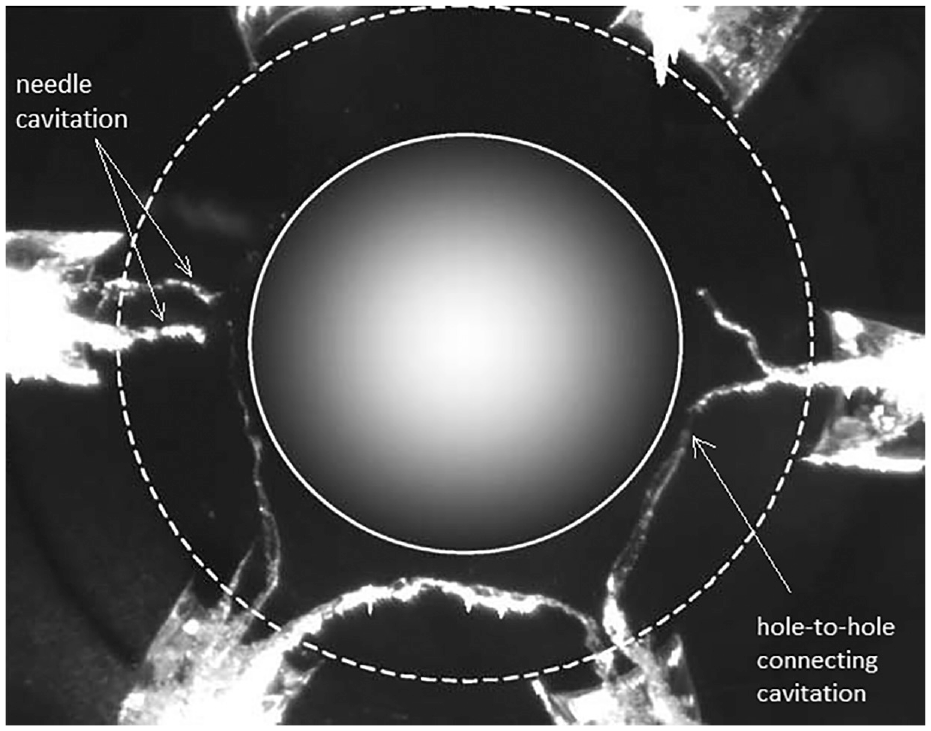
High-speed digital still image of fuel injector from the bottom, showing “hole to hole” connecting string cavitation and vortex cavitation emerging from the needle wall facing the injector hole.
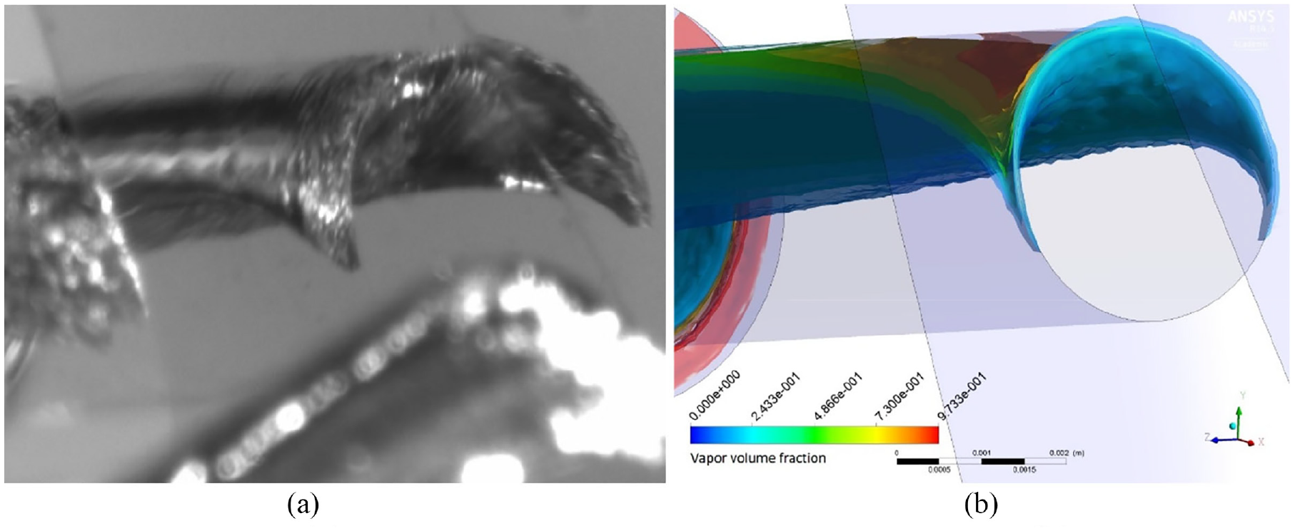
The simulations are finally qualitatively assessed by comparing the predicted vapor volume fraction with high-speed CCD images of cavitation reported by Afzal et al. 5 in the same setup as the current injector geometry and under similar operating conditions. A comparison between the side view of a still image of cavitation inside the injector hole and predicted vapor volume fraction in Figure 12(a) and (b) at the same needle lift and cavitation number indicate good agreements achieved in capturing similar cavitation structures like its initiation and formation at the upper edge of the nozzle, its size and shape, and that it remains attached to the injector wall as it travels downstream. It can also be seen from the comparison of Figure 13(a) and (b) that CFD simulations have resulted in the prediction of a similar horseshoe-shaped profile of vapor distribution as of the experiment.
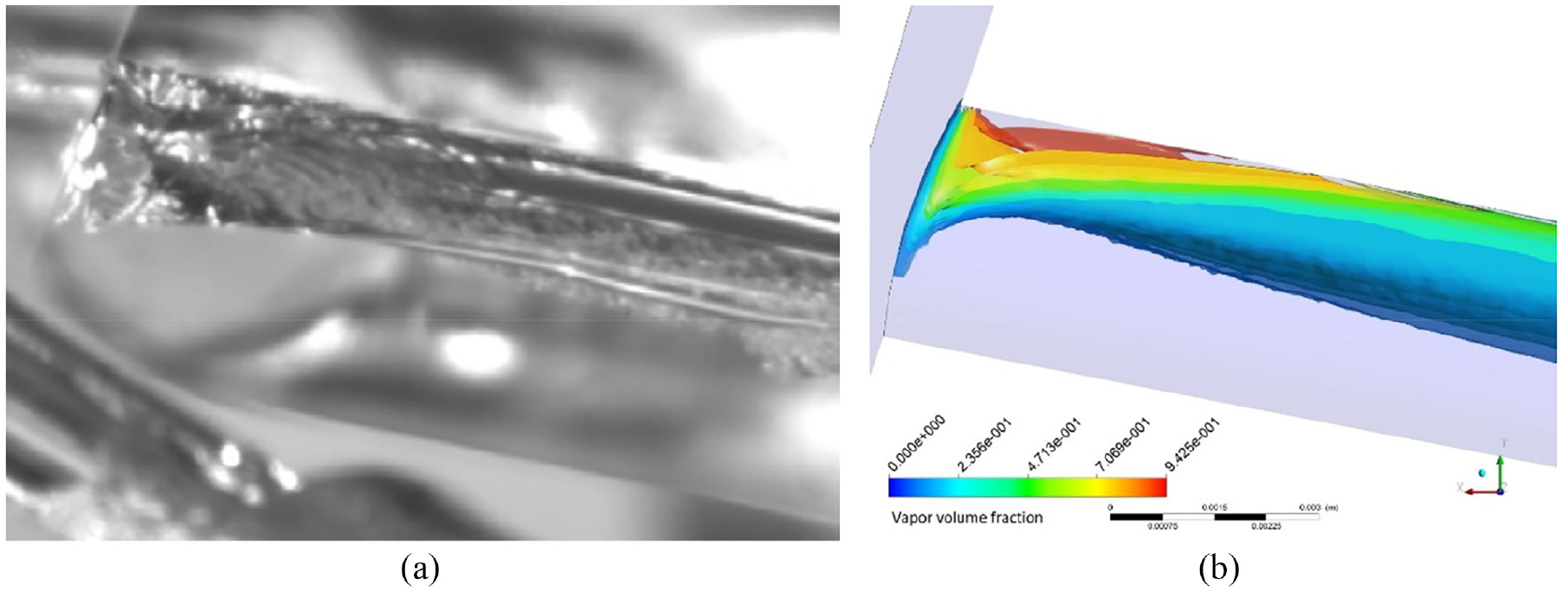
(a) Still photograph (side view) of the geometry induced cavitation formed at the upper edge of the nozzle originating at the entrance edge and traveling downstream flow travels downstream, the image indicates cavitation remains attached to the injector wall, source: Afzal et al. 5 and (b) isosurface of void fraction prediction at CN = 4.57 and nominal needle lift of 6.00 mm.
(a) Still photograph of the geometry induced cavitation formed at the upper edge of the entrance of the injector hole and traveling downstream, the image indicates cavitation remains near the injector wall and show the horseshoe appearance of cavitation, source: Afzal et al. 5 and (b) isosurface of void fraction prediction at CN = 4.57 and nominal needle lift of 6.00 mm.
Conclusions
In this study, the internal flow in a diesel multi-hole fuel injector reminiscent of ones used in heavy-duty trucks is simulated and analyzed at non-cavitating and cavitating conditions using the RANS approach that was found to be most appropriate due to its ability to predict such flows efficiently with competent accuracy and much lesser computational cost and time. ZGB cavitation model was used with the realizable k-epsilon turbulent model; the liquid compressibility was modeled using the Tait equation, and the vapor compressibility was modeled using the ideal gas law. The accuracy of simulations is assessed by comparing the predicted mean axial and RMS velocity with that of experimental measurement. At the cavitating flow conditions, the predicted cavitation void is also compared with the high-speed digital image. The following are a summary of the main findings and contributions of the current research study:
The comparison of predictions at non-cavitating conditions showed good agreement with measured values of mean and RMS velocity. RMS prediction results also showed an increase in magnitude with an increase in mesh density. At cavitating conditions, the comparison of predicted mean velocity results with experimental data also showed good agreement, while the RMS velocity results were to some extent underpredicted but followed accurately the trend of the measured values.
The prediction results showed no appreciable differences in mean and RMS velocities on assuming the phases to be compressible or incompressible, suggesting that the influence of compressibility on mean and RMS velocity, within the calculated CN range, is not evident.
The qualitative comparisons of predicted cavitation vapor volume with experimentally recorded high-speed digital images at the same operating conditions showed a very good agreement.
The flow field analysis, in particular, of vorticity, showed good similarities with experimentally recorded high-speed digital images of vortical cavitating structures present in the multi-hole fuel injector nozzle. The first one was “hole-to-hole” connecting vortices, and the second one was “double counter-rotating” vortices emerging from the needle wall and entering into the injector hole facing it.
Footnotes
Appendix
Acknowledgements
The first author would like to thank the City, University of London for the full scholarship and bursary for this research. The authors would also like to appreciate the help provided by Mr. Chris Marshall for using the university cluster.
Author contributions
A.K.: methodology, software, formal analysis, writing – original draft, writing – review and editing; J.M.N.: conceptualization writing and preparation – original draft, writing – review and editing, supervision, funding acquisition; A.G.: conceptualization, writing – review and editing, supervision. All authors have read and agreed to the published version of the manuscript.
Declaration of conflicting interests
The author(s) declared no potential conflicts of interest with respect to the research, authorship, and/or publication of this article.
Funding
The author(s) received no financial support for the research, authorship, and/or publication of this article.