Sage Journals: Discover world-class research

Abstract

A novel calibration methodology is presented to accurately predict the fundamental characteristics of high-pressure fuel sprays for Gasoline Direct Injection (GDI) applications. The model was developed within the Siemens Simcenter STAR-CD 3D CFD software environment and used the Lagrangian–Eulerian solution scheme. The simulations were carried out based on a quiescent, constant volume, computational vessel to reproduce the real spray testing environment. A combination of statistic and optimisation methods was used for spray model selection and calibration and the process was supported by a wide range of experimental data. A comparative study was conducted between the two most commonly used models for fuel atomisation: Kelvin–Helmholtz/Rayleigh–Taylor (KH–RT) and Reitz–Diwakar (RD) break-up models. The Rosin–Rammler (RR) mono-modal droplet size distribution was tuned to assign initial spray characteristics at the critical nozzle exit location. A half factorial design was used to reveal how the various model calibration factors influence the spray properties, leading to the selection of the dominant ones. Numerical simulations of the injection process were carried out based on space-filling Design of Experiment (DoE) schedules, which used the dominant factors as input variables. Statistical regression and nested optimisation procedures were then applied to define the optimal levels of the model calibration factors. The method aims to give an alternative to the widely used trial-and-error approach and unveils the correlation between calibration factors and spray characteristics. The results show the importance of the initial droplet size distribution and secondary break-up coefficients to accurately calibrate the entire spray process. RD outperformed KH–RT in terms of prediction when comparing numerical spray tip penetration and droplet size characteristics to the experimental counterparts. The calibrated spray model was able to correctly predict the spray properties over a wide range of injection pressure. The work presented in this paper is part of the APC6 DYNAMO project led by Ford Motor Company.

Keywords

Gasoline direct injection spray modelling break-up model statistical and optimisation techniques computational fluid dynamics STAR-CD spray model calibration high-pressure fuel injection

Introduction

Over the last few years, spark-ignited Gasoline Direct Injection (GDI) engines have become the benchmark for modern light-duty vehicle applications. The possibility to operate either in homogeneous or stratified charge mode gives them high efficiency^1–3 and the versatility required to cope efficiently with the vast majority of driving scenarios.⁴ In addition to advanced fuelling strategies, the GDI technology is often combined with turbo-charging and Variable Valve Timing (VVT) within the down-sized philosophy which brings further thermal efficiency gains and emissions reduction.^2,5 The stable car market penetration of GDI solutions has led to the rapid development of high-pressure fuel injection systems with maximum injection pressure steadily rising to 800 bar.⁶ Moreover, forecasts indicate how almost 60% of global engine production will adopt an in-cylinder fuel injection system by 2024.⁷ Despite the promising scenario, GDI engines are still affected by peculiar issues. In particular, in-cylinder air-fuel mixture mal-distribution occurs due to a relatively short interval between injection and ignition. The resulting presence of rich mixture-pockets before and during combustion has been proved to intensify the formation and emission of Particulate Matter (PM).^8–11 Around 240,000 people die each year with diseases correlated with PM emitted by motor vehicles.¹² While higher fuel injection pressure speeds up the mixing process through stronger droplets atomisation, the consequent deeper spray penetration potentially leads to spray-to-wall impingement, especially in the context of small-capacity cylinders. The likely liquid film deposition, in certain operating conditions (e.g. cold start and warm-up phases; high load), may develop into pool-fire – another significant source of PM, and further contribute to mixture mal-distribution.^10,13

Computational Fluid Dynamics (CFD) software capabilities and High-Performance Computing (HPC) can be used to support the development of high-pressure fuel spray systems. High-fidelity 3D CFD models of the GDI engine injection process, based on phenomenological models validated against experimental data, have demonstrated the ability to predict relevant spray characteristics reliably.^14,15 In particular, the models can reveal characteristics that are difficult or impossible to record in certain experimental conditions and/or locations, for example, close to nozzle holes and generally within high fuel density regions. The approach used for model calibration is of importance, and often model ‘tuning’ is based on a limiting trial-and-error methodology which inherently lacks robustness.¹⁶ Despite good overall predictions, this method describes the spray process only partially and it is condition-specific rather than general. The rigorous approach outlined in this paper, based on statistical analysis and optimisation techniques, not only leads to a robust spray process prediction but also represents a generalised calibration approach extendable to other phenomenological or semi-fundamental models. The current trends in engine and automotive research and development, as outlined by UK Automotive Council Roadmap,¹⁷ clearly show that imparting robustness and generality to predictive model will support the necessary shift from prototype testing to model-based development within the industry, reducing costs and time-to-market. Improving the current knowledge of the fuel sprays through modelling also constitutes a cost-effective avenue to contribute to reducing the impact of modern petrol engines on the environment and human health.

Wang et al.¹⁸ compared the performance of Reitz–Diwakar (RD) and Kelvin–Helmholtz/Rayleigh–Taylor (KH–RT) models to predict isooctane high-pressure sprays from an outward-opening injector in a quiescent vessel. The models were calibrated selecting three levels for the most influential calibration factors. The initial droplets size distribution was supplied by means of Rosin–Rammler (RR) equation with fixed calibration factors for all cases investigated. RD model produced the best results, with one set of calibration factors able to capture the behaviour of the real injector for the two vessel back-pressures investigated. On the contrary, the combination of central flow motion and the stronger break-up produced by KH–RT model led to abnormal spray penetration and morphology. Braga et al.¹⁹ used a similar calibration methodology to predict the high-pressure injection of ethanol from a seven-hole injector using the KH–RT instability model. Four levels for each calibration factor were chosen and their effect on spray penetration characteristics analysed in comparison with experimental data. The model prediction capabilities slightly improved with the number of points selected to describe the typical trapezoidal fuel mass flow rate versus time profile. The RT droplet diameter break-up factor and the KH break-up time were the parameters showing greater influence on spray Sauter Mean Diameter (SMD), penetration and morphology, highlighting the importance of fuel droplet size to augment the predictive potentials. Ho Teng²⁰ developed empirical equations based on experimental fuel Mass Flow Rate (MFR) to predict fuel spray characteristics from a GDI multi-hole injector. For a fully spatially developed spray, that is, later injection stage, the droplet size distribution was reproduced by a cumulative RR function that allowed predicting SMD and droplet diameter corresponding to a particular volume fraction. Increasing the injection pressure, the cumulative curve shifted towards smaller diameters as a consequence of enhanced atomisation. Costa et al.²¹ adopted a statistical methodology for the calibration of spray models for GDI engine applications. The initial droplet size distribution at nozzle exit was predicted according to a log-normal Probability Distribution Function (PDF), with mode dependent on both gasoline and ambient properties. The variance of the distribution was selected as first tuning parameter. For the droplet break-up process, the authors selected the Huh and Gosman model with break-up time as second calibration parameter. For a given injection pressure, DoE-based variance and break-up factor were used as simulation inputs, along with the experimental profile of fuel MFR. An iterative process was implemented to determine, within the DoE spaces, the tuning factors values able to minimise the squared error between experimental and numerical spray penetration length. Results indicated the fundamental influence of injection pressure on initial droplet distribution and size, and how increasing the injection pressure resulted in physically acceptable behaviour with narrower distribution and higher probability of smaller diameter. Perini and Reitz²² utilised a multi-objective Non-dominated Sorting Genetic Algorithm II (NSGA-II) to interpret the correlations existing among model calibration factors and to select the optimal set to reproduce a diesel spray process. A blob injection model was combined with the KH–RT model within a constant volume 3D domain. A total of six calibration factors were investigated: three for the KH–RT break-up model and the other three related to the sub-grid near-nozzle flow model. Once break-up occurred, a RR distribution centred on perturbation length in the liquid-gas interface was used to select the new droplet size. The five objective functions were related to vapour/liquid penetration, liquid penetration in the ballistic region and air-fuel mixture fraction over several equally spaced locations along the domain. The Pareto front analysis demonstrated how both liquid and vapour penetration are well captured with similar values of calibration factors. The sensitivity analysis of the calibration constants revealed their influence on the uni-dimensional objective functions but did not provide clarity on how each factor influences the modelled spray behaviour. For example, another study found a linear correlation between the time scale of the secondary break-up and the equivalence ratio, proving the connection between calibration factors and fundamental spray characteristics such as SMD.²³

In the present work, a statistical and nested optimisation procedure has been developed to calibrate the spray model of a high-pressure injector currently used in a modern small-capacity spray-guided GDI engine. The initial, nozzle exit, droplet size distribution is reproduced with a mono-modal RR equation. Once computational parcels/droplets are injected inside the 3D CFD domain, the atomisation process was analysed with both KH–RT and RD break-up models, selecting the best scheme that would reproduce the available experimental data. The latter included spray-tip penetration, reconstructed droplet size distribution function at 50 mm down the injector and spray morphology. A half factorial screening method was used to enable the selection of only the most significant calibration factors for optimisation, reducing in this way the dimensionality of the problem. The paper outlines the first steps of a larger investigation that aims to develop a comprehensive and generalised set of modelling methodologies to support the development of the next generation of highly efficient, Ultra Low Emission (ULE) GDI engines. Improving the prediction of the fuel injection process is a fundamental step that enables realistic predictions of air-fuel mixing, combustion and pollutants formation. The paper is structured as follow: the first part describes the experimental test procedures to obtain spray data and introduces equations and models utilised to predict the injection process, with special insight on statistical and optimisation approaches for model calibration; the second part deals with model selection and the results of model calibration over a wide range of injection pressure.

Methodology

Experimental setup for spray data acquisition

This work is based on a modern five-hole GDI injector capable of injection pressure above 300 bar. The experimental data have been collected by Ford Vehicle Evaluation & Verification (VEV) Powertrain and Fuel Subsystem Laboratory, USA. The data covered the main spray characteristics used in the vast majority of similar modelling studies.^14,16,19 A schematic drawing of the nozzle is presented in Figure 1 where S_ϑ is the circular distance between two near holes, D_i is the geometric hole diameter that for the proposed injector was 180 µm, R is the hole distance from the centre and ϑ is the angular distance between two near holes. 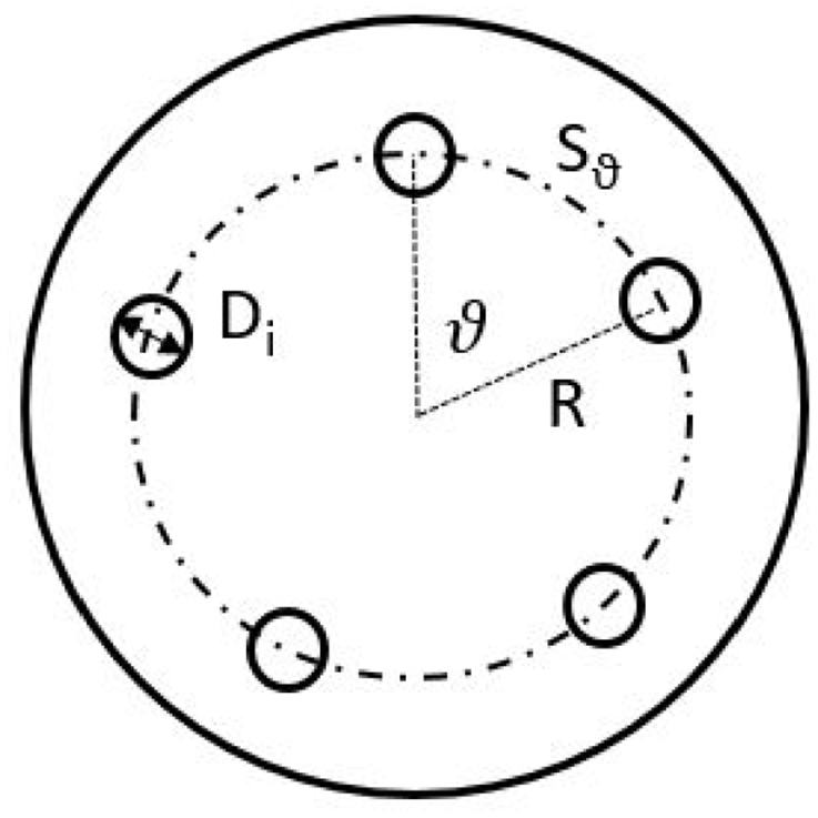According to Khan et al.,²⁴ the limiting condition $S_{θ} / D_{i} > 3.5$ prevent the spray plumes from collapsing during the injection, mitigating the phenomena of flash boiling. The injector used in this study is a ‘wide-hole’ configuration, which respects this $S_{θ} / D_{i}$ condition.

Figure 1.

Schematic representation of the tip view for a five-hole injector.

A detailed account of the test setup and experimental methodology is beyond the scope of this study. Hence, only a brief description is introduced here. Four different types of tests were conducted for the spray characterisation:

Spray pattern visualisation test

High-speed imaging test

Laser diffraction droplet size test

Fuel MFR test

All the tests used n-heptane as indicated by SAE J2715 recommended practices.²⁵ N-heptane is preferred to isooctane being less volatile and hence safer to be used in a laboratory while maintaining similar properties. The visualisation test of the spray pattern aimed to obtain the spray footprint to understand the distribution of the plumes on a reference plane. The test was carried out at 35 bar injection pressure and 1 bar back-pressure, mounting the injector 50 mm above the calligraphy paper. The data collected were fundamental for the spray geometry modelling, enhancing the prediction capability of plumes geometry and the coordinate system of the injector holes. The high speed-imaging test provided information on spray morphology and penetration. The injector was placed inside a quiescent vessel with two optical accesses perpendicular to each other. The injection pressure was varied from 50 to 250 bar with 1 bar back-pressure. The spray tip penetration was calculated as the axial distance between the injector nozzle and the point reached by the 95% of droplets injected by mass.²⁶ The laser diffraction droplet size test repeated the operating conditions investigated in the previous test and used a laser beam traversing two spray plumes to evaluate the liquid droplet dimension. This test was used to obtain precise values of droplets SMD, D_v₁₀ and D_v₉₀ on a plane 50 mm down the injector. The use of a reference plane at a certain distance is a common practice to overcome the difficulties of optical investigations close to nozzles where higher pixel density can introduce inaccuracy.²⁵ For the fuel MFR test, a constant volume chamber was used to record the fuel flow shot to shot variation in combination with a Coriolis flowmeter. The averaged results were provided for a range of injection pulse widths.

Model description and implementation

Spray simulations have been developed within the Siemens Simcenter STAR-CD CFD package v4.32, using a coupled Lagrangian/Eulerian approach.^27,28 Discretised droplets (fuel) were introduced in a continuous matter (nitrogen) and solved by means of Reynolds–averaged Navier–Stokes (RANS) equations. Turbulence generated by the interacting fluids was treated by means of k–ε RNG turbulence model. The multi-dimensional second-order Monotone Advection and Reconstruction Scheme (MARS) was adopted to handle flow characteristics within the computational cells. Momentum-pressure equations and all the other discretised equations were solved by means of Numerical time-step Pressure-Implicit with Splitting of Operators (PISO) algorithm. The Lagrangian phase was modelled with the ‘parcel approach’ which consists of a group of droplets described with identical properties. No interactions occurred between spray plumes and walls and hence no liquid film model was implemented. Temperature dependent thermo-physical properties from the NIST tables were used for all gaseous and liquid components. The collision model was deactivated because the sub-model did not improve the prediction of the spray pattern so much to justify increased simulation time. As reported in the previous section, the injector configuration prevented the phenomena of flash boiling therefore the related sub-model was deactivated.

The spray process is summarised as a combination of three components: liquid fuel, fuel vapour and ambient matter. They constantly interact defining internal and external spray characteristics.²⁰ The size of the droplets and their distribution can be classified as internal parameters, while tip penetration and spray morphology as external parameters. The proper prediction of all parameters is fundamental to capturing mixture formation.²⁹

A quiescent, constant volume, cylindrical domain was created to reproduce the experimental test setup. The geometry featured a bottom pressure boundary and a wide wall configuration to minimise spray-wall influence on spray characteristics. The injector’s holes were positioned at the top of the vessel, centrally. A central cross-section of the vessel is presented in Figure 2; here, it is possible to appreciate the four levels of mesh refinement, with the finest cell dimension of 0.5 mm to maximise the fluid-dynamic prediction performance in the near-nozzle region.^15,30 The experimental penetration values and images facilitated the optimisation of the mesh. The selected levels of refinement and shape were a trade-off between model prediction accuracy and computational cost, with the finest dimension corresponding to the mesh size in the injector region of the combustion chamber for typical GDI engine CFD modelling. Table 1 summarises the main features of the virtual vessel. Software implementation for this study included a subroutine that allowed the calculation of spray penetration length and droplet size distribution at every time step on a plane 50 mm down the injector to reproduce the experimental setup.

Figure 2.

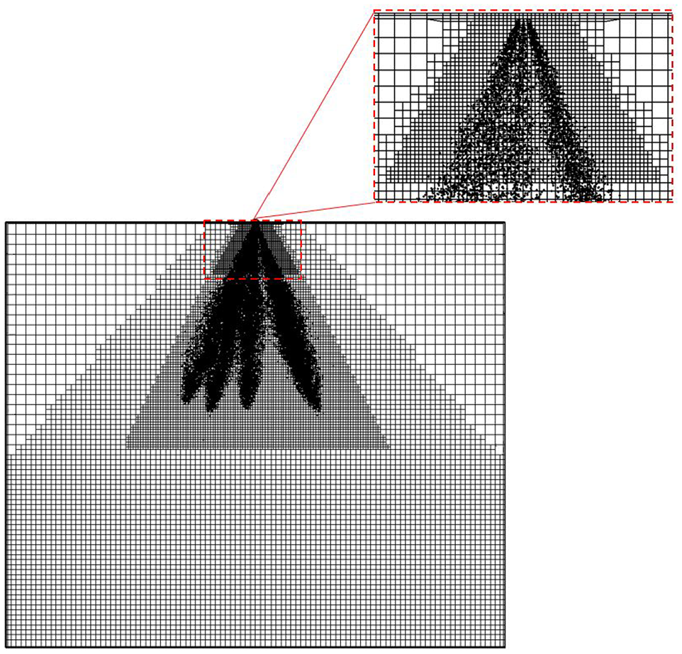
Cross-section of the quiescent vessel mesh and zoom in on the most refined region.

Table 1.

Modelled quiescent vessel characteristics and setup.

Vessel dimension	D = 200 mm, L = 170 mm
Mesh refinement	3.5 → 2 → 1 → 0.5 mm
Number of cells	800,000
Bottom face	Pressure boundary
Top face plus side	Adiabatic wall
Back-pressure (abs.)	1 bar
Vessel temperature	293 K
Vessel fluid	Nitrogen
Physical run-time	2 ms

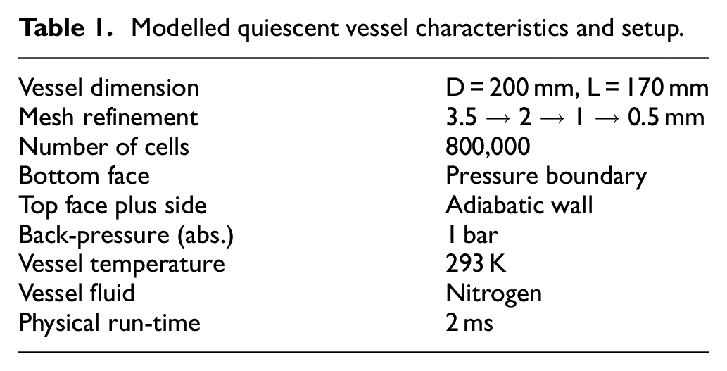
Figure 3 shows the comparison between the experimental and simplified fuel MFR for three injection pressure, from 50 to 250 bar. The simplified profile was computed from the experimental counterpart minimising the error between the area under the trapezoid and the experimental total mass injected and following the variation of opening/closing ramps with injection pressure. The procedure simplified the model setup and did not degrade the prediction capability. Using the available experimental data, the same injection profile was adopted for each hole. A discharge coefficient was estimated from the Bernoulli equation and varied with the injection pressure. The coefficients were applied to the geometrical diameter of the holes and reduced their dimension to a D_effective that changed from 132 to 128 µm going from 50 up to 250 bar. The proposed approach omitted the investigation of the nozzle internal flow and imposed an initial droplet distribution that disintegrated following well-known break-up models. Even if the generality of the overall spray model characterisation may be reduced, the gain in terms of computational time can justify the suggested approach as demonstrated in similar studies.^15,18,22

Figure 3.

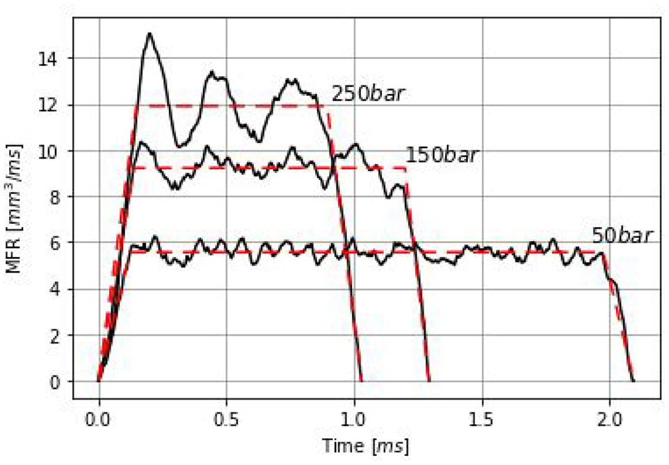
Comparison between experimental (black) and simplified (red) fuel mass flow rate versus time profiles, for three levels of injection pressure.

An understanding of the phenomenological model equations and the influence of calibration factors on numerical responses is necessary for the development of robust spray models.

The RR cumulative function, equation (1), was selected to characterise both the initial droplet distribution at the nozzle exits within the CFD model and the experimental spray droplets size distribution on a reference plane 50 mm down the nozzle:

Q = 1 - \exp {[- \frac{D}{X}]}^{q}

(1)

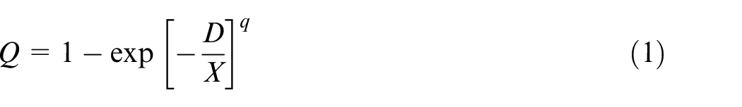
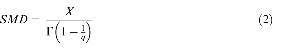
In equation (1), Q is the total volume fraction of droplets with a diameter up to D; X and q are model calibration factors. For D equal to X, Q takes the value 0.632 and hence X represents the reference diameter for which 63.2% of the total liquid volume exists as droplets with a diameter smaller than X. The exponent q indicates the spread of size distribution, with narrower distribution for greater values. Despite this function not being able to describe multi-modal distributions, the RR model has been proven to consistently predict the droplet size distribution of GDI injectors.³¹ The SMD can be obtained as a function of X and q,²⁰ where the latter is defined as an argument of the gamma function Γ, as follows:

SMD = \frac{X}{Γ (1 - \frac{1}{q})}

(2)

Combining equations (1) and (2):

\frac{D}{SMD} = - {[\ln (1 - Q)]}^{\frac{1}{q}} Γ (1 - \frac{1}{q})

(3)

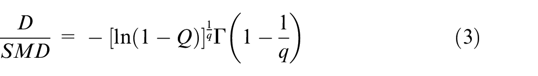
Equation (3) is of general nature, being able to correlate different volume fractions for a given droplet distribution. This permits the evaluation of the distribution spread. For example, for Q = 0.9 →D = D_v90 and knowing the ratio between the latter and SMD it is possible to obtain q. The same equation can be used to obtain D_v10.

The SMD is a crucial spray parameter. It is often convenient to represent SMD using a continuous probability density function (PDF), which summarises the droplet distribution.^20,32 Knowing X and q, the PDF is obtained from equation (1) as the numerical derivative of Q with respect to D:

{(\frac{dQ}{dD})}_{i} = \frac{(Q_{i + 1} - Q_{i - 1})}{(D_{i + 1} - D_{i - 1})}

(4)

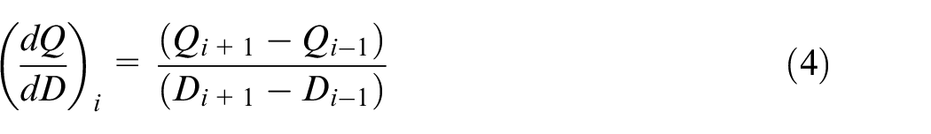
Equations (2)–(4) were used to reconstruct the droplet distribution from experimental spray on a plane 50 mm down the injector.

Starting from the RR initial drop distribution, parcel/parent droplets are introduced in the 3D domain. To recreate the spray atomisation process, parent droplet break-up occurs due to forces produced by their interactions with the continuous gas phase. The resulting instabilities generate child droplets that can be predicted, as for the RR, with phenomenological constant-sensitive models. 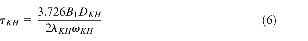The two most common break-up models for GDI applications have been analysed in this work: KH–RT³³ and RD break-up models.³⁴ The KH–RT is a hybrid model formed by the combination of two sub-models, both based on instabilities growing within the liquid-gas interface. For the KH model, the instability is generated by aerodynamic forces. The RT model, instead, predicts the break-up as a result of droplet deceleration and density difference between the two involved fluids. For each parcel injected, the two models evaluate the break-up simultaneously, with the fastest dominating over the slowest and hence used as break-up mechanism at each time step. Both KH and RT models depend on two calibration constants that influence the child droplet dimension and the break-up time rate. Equations (5) and (6) indicate the diameter of the child droplet D_KH and break-up time $τ_{KH}$ for the KH model, respectively:

D_{KH} = 2 B_{0} λ_{KH}

(5)

τ_{KH} = \frac{3.726 B_{1} D_{KH}}{2 λ_{KH} ω_{KH}}

(6)

In these equations, $λ_{KH}$ is the instability wavelength, $ω_{KH}$ is the growth rate of the fastest growing wave and B₀ and B₁ are the calibration factors. When the parent droplet assumes a radius equal to the perturbation wavelength, the break-up will produce a new parent and a child droplet. B₁ depends on turbulence and/or cavitation phenomena within the injector and has a strong effect on fuel spray evolution.³⁵ The RT model has a similar structure, both in terms of equation form and calibration factors. Equations (7) and (8) represent the diameter D_RT of the child droplet and break-up time $τ_{RT}$ for the RT model, respectively:

D_{RT} = C_{3} λ_{RT}

(7)

τ_{RT} = \frac{C_{t}}{ω_{RT}}

(8)

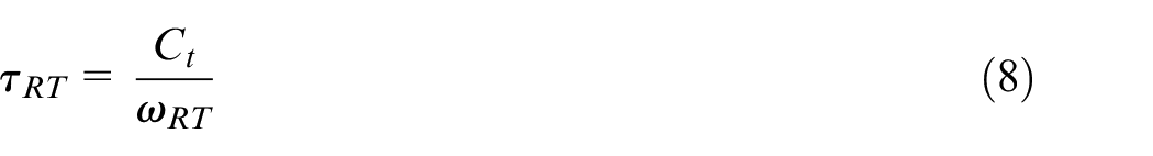
In these equations, C₃ and C_t are the calibration factors.

The RD model^28,34 predicts the break-up based on two mechanisms: ‘bag break-up’, due to pressure instability and expansion of the droplet towards lower pressure region, with subsequent separation of the child droplet; and ‘stripping break-up’, which produces the child droplet by means of a shearing process from the parent droplet surface. The following equations outline the role of each break-up mechanism and their correlation with calibration factors. The Weber number threshold value for bag break-up is

We \equiv \frac{ρ {| u - u_{d} |}^{2} D_{d}}{2 σ_{d}} \geq C_{b 1}

(9)

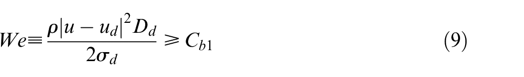
where u and ρ are the gas velocity vector and density, respectively; D_d is the droplet diameter, $σ_{d}$ the surface tension and $σ_{d}$ the velocity vector. C_b1 is a tuning parameter; if the droplet Weber number is smaller or equal to C_b₁, then the droplet is stable; otherwise break-up will take place. The characteristic break-up time rate τ_b is related to the same parameters as follows:

τ_{b} = \frac{C_{b 2} ρ_{d}^{\frac{1}{2}} D_{d}^{\frac{3}{2}}}{4 σ_{d}^{\frac{1}{2}}}

(10)

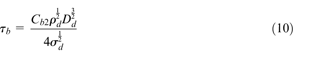
In this equation, C_b₂ is another calibration factor and ρ_d is the droplet density.

The stripping break-up threshold involves the droplet Reynolds number to take account of the dynamic viscosity as follows:

\frac{We}{\sqrt{R e_{d}}} \geq C_{s 1}

(11)

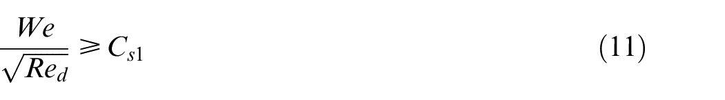
In this equation, C_s₁ is the tuning parameter with a similar role as C_b₁. The stripping break-up time rate is given by:

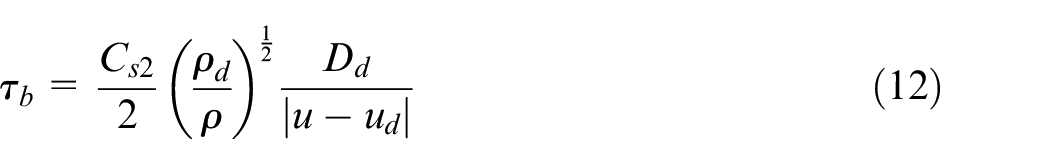
τ_{b} = \frac{C_{s 2}}{2} {(\frac{ρ_{d}}{ρ})}^{\frac{1}{2}} \frac{D_{d}}{| u - u_{d} |}

(12)

where C_s₂ is the fourth calibration factor of the model.

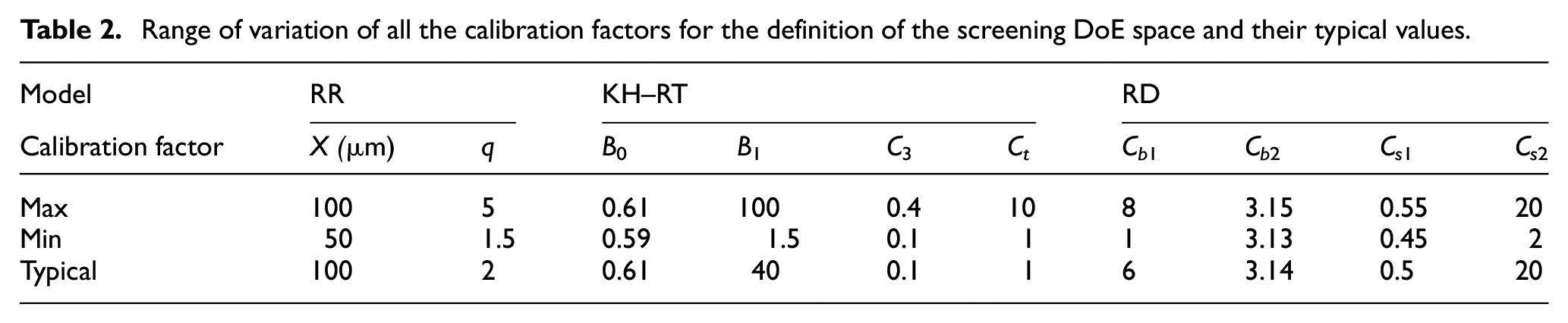
The typical ranges of variation for the calibration factors are summarised in Table 2 based on the most relevant literature^15,18,19 and the Authors’ previous experience.^8,10 In particular, the X range was selected considering the diameter of the holes and studying the experimental SMD for all the injection pressure tested. Identifying operational ranges is the first step for the factors screening and selection process, as described in detail in the following paragraph.

Table 2.

Range of variation of all the calibration factors for the definition of the screening DoE space and their typical values.

Model	RR		KH–RT				RD
Calibration factor	X (µm)	q	B ₀	B ₁	C ₃	C_t	C_b ₁	C_b ₂	C_s ₁	C_s ₂
Max	100	5	0.61	100	0.4	10	8	3.15	0.55	20
Min	50	1.5	0.59	1.5	0.1	1	1	3.13	0.45	2
Typical	100	2	0.61	40	0.1	1	6	3.14	0.5	20

Models selection and calibration

The block diagram shown in Figure 4 summarises the model calibration procedure, which is reported in detail in the following sections.

Figure 4.

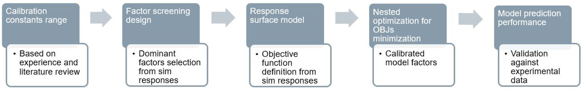
Workflow for the proposed calibration factor screening and optimisation process.

Two model combinations, RR + RD and RR + KHRT, were initially considered at a fuel injection pressure of 150 for the screening process. The workflow depicted in Figure 4 was applied to both and the results were compared in terms of their ability to match experimental observations at two injection pressures (150 and 250 bar). Six calibration factors, as reported in Table 2, were associated with each model combination. Rather than carrying out numerically intensive optimisation procedures in all six factors, a screening process was used to determine the dominant ones. A more extensive response surface experimental design, based on a space-filling principle (Halton sequence), was then conducted in the dominant factors identified by the screening process. The purpose of this approach was to build fast spatial statistical models to subsequently seed a nested optimisation process to determine the final calibration factor settings.

Factor screening process

The objective was to determine the dominant factors and two-term interactions only. This approach significantly reduced the overall number of CFD simulations required for spray model calibration. The methodology is commonly used in statistical experimentation.³⁶ A test matrix with $2_{VI}^{6 - 1}$ = 32 calibration factor combinations was used. The defining word for this design was $I = ABCDEF$ (i.e. calibration constants for the RR model plus the four related to each break-up model) with a resolution VI.³⁶ Consequently, it was possible to quantify significant two-term interactions as well as the main effects of the respective factors. The corresponding regression equation was:

y = b_{0} + \sum_{i = 1}^{6} x_{i} b_{i} + \sum_{i = 1}^{5} \sum_{j = i + 1}^{6} x_{i} x_{j} b_{ij}

(13)

Montgomery³⁶ provides extensive tables of $2^{p - k}$ fractional factorial designs, with designs in up to $p = 15$ factors in 16 runs. The sparsity of effects principle³⁷ suggests system responses are dominated by main effects and low order interactions. Therefore, a main effect is much more likely to be active than, for example, a five-term interaction. A half factorial design was selected because considered the best trade-off between accuracy of the information obtained and computational time. The calibration factor performances on the CFD simulation responses were investigated in terms of SMD on a plane 50 mm down the nozzle, and spray penetration at 0.8 ms after start of injection (ASOI). The former was selected to align the numerical results with the experimental counterpart. The latter to account for the spatial and temporal evolution of spray near the maximum penetration.

Response surface design and modelling

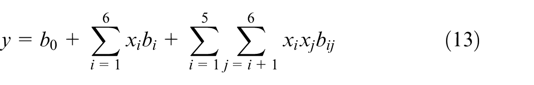
To seed the optimisation process yielding the final calibration parameters, a more exact model describing the complex behaviour of the response metrics over the factor space was required in comparison with the one defined with equation (13). As the optimisation algorithm requires many evaluations, the actual CFD simulation models cannot be used to calculate the appropriate cost function as the evaluation time would be too long. Consequently, a surrogate model approach was adopted to provide fast prediction (obtained generally in a fraction of a second) of the responses not investigated with a CFD simulation. The surrogate of a detailed computer simulation model is called a meta-model.³⁸ The underlying concepts are described in Figure 5 for a function of two variables (factors). Initially, a DoE was developed, generating a list of points at which CFD simulations were carried out. A variety of suitable techniques, most often predicated on space-filling principles, appear in the literature.^39–42 The accuracy afforded by the meta-model in interpolating among previously untried configurations depends on the design, particularly the number and distribution of points, as well as the interpolating function itself.

Figure 5.

The concept of meta-modelling for a response depending on two design variables.³⁸

Definition of response metrics and optimisation process

The CFD results, from DOE analysis, in terms of penetration and SMD, were used to construct the objective function 1 (OBJ1) and 2 (OBJ2):

OBJ 1 = \frac{1}{t} \int_{0}^{t} {(\frac{p_{num} (τ) - p_{\exp} (τ)}{p_{\exp} (τ)})}^{2} d τ

(14)

OBJ 2 = \frac{1}{D} \int_{0}^{D} {(\frac{c_{num} (δ) - c_{\exp} (δ)}{c_{\exp} (δ)})}^{2} d δ

(15)

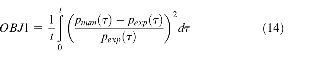
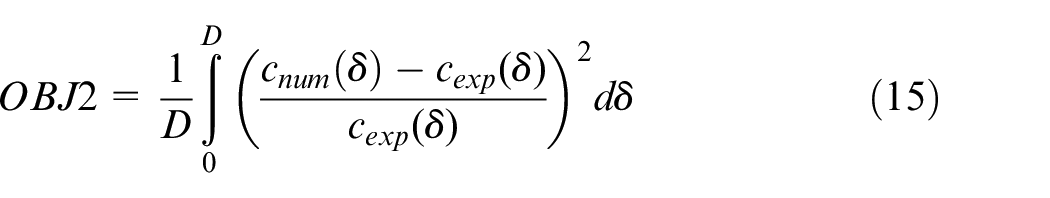
Equations (14) and (15) describe the level of prediction performance of the model in terms of liquid penetration and cumulative droplet dimension, respectively. The objective functions were designed as a squared deviation of the numerical values from the experimental data. In particular, equation (14) computes the squared error between the instantaneous numerical penetration p_num and the experimental counterpart p_exp as a function of time τ. Equation (15) is defined with a similar approach and it evaluates the squared error between the numerical cumulative curve c_num and the experimental value c_exp of droplet diameter δ. The curves were obtained at 50 mm down the nozzle and 0.8 ms ASOI. The use of both penetration and cumulative droplet dimensions to characterise the gasoline spray is aligned with the SAE J2715 recommended practices.²⁵

For each injection pressure, a nested optimisation process was performed with a population of 2000 and 500 interactions. OBJ2 was selected to be minimised imposing a constraint on OBJ1. Since the tip penetration is more dependent on droplet velocity, that is, fuel MFR, the calibration factors were selected giving more weight to the prediction of droplet dimensions and hence OBJ2. A minimum threshold error was imposed on OBJ1. The threshold influenced the solutions of the optimiser in terms of calibrated factors. Consequently, an iterative process was performed to select, for each injection pressure, an OBJ1 threshold to provide the best solutions that follow the variation of the spray characteristics observed experimentally. The analysis of these results enabled, as reported in the following section, to select the model combination RR + RD as the most suitable for modelling sprays in high-pressure GDI applications.

Results and discussions

Factorial screening and spray model selection

Figure 6 presents the absolute regression coefficients b, for both the SMD and spray penetration at 0.8 ms ASOI, for the RR + RD model combination. The R² values for these regressions were 0.9943 and 0.9999, respectively. Both models were good facsimiles for the simulation data. The taller the bar, the more influential the factor was in explaining the observed behaviour in the response. Considering the SMD bar chart, the largest effects in descending order were X, C_b₁ and C_b₁X. 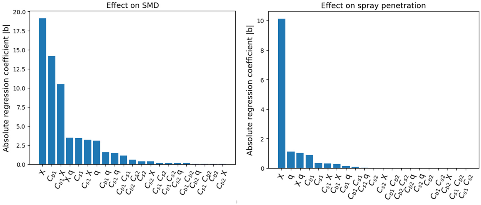Noticeably, the control obtained over droplet dimensions with X and the onset of the bag break-up with C_b₁ largely modify the SMD ( $| b | > 10)$ while the other calibration constants, that control the spread of the droplet distribution (q), the bag break-up rapidity (C_b₂) and the stripping mechanism at higher Weber numbers (C_s₁ and C_s₂), have a smaller impact ( $| b | < 5)$ . A second SMD regression against the three dominant factors exhibits an R² of 0.9250. Consequently, it was possible to accept X, C_b₁ and their interaction C_b₁X as the most influential factors.

Figure 6.

Absolute regression coefficients for the SMD and penetration at 0.8 ms ASOI least squares analysis for the RR + RD combination. The higher the bar the more influential the factor.

Considering the penetration response analysis, the most influential factor was X, which stands out against the remaining factors. The penetration is primarily affected by the droplet velocity (i.e. MFR profile – a fixed value for this screening analysis) and secondarily by the droplet initial dimensions that can be widely adjusted with X and q. The other calibration constants seem to have low to none effect also when in combination with the more influential X or q. As shown for the SMD study, the bag break-up factor stands out against the stripping process with their constants generally more significant. A follow-up regression analysis in X alone exhibits an R² value of 0.9672. The analysis provided evidence that for the RR + RD model combination the factors X and C_b₁ are sufficient to correctly tune the spray characteristics.

Figure 7 presents a plot of the corresponding absolute regression coefficients for the RR + KHRT model combination. The R² values for the SMD and penetration models were 0.9690 and 0.9387, respectively. This suggested that the regressions were adequately explanatory for the simulation data. For the SMD bar chart, the most influential explanatory factors were: C₃, X, C₃X, followed by q and C₃q. Similarly to the previous model combination, the SMD seems mainly influenced by a break-up coefficient and the initial droplet distribution controlled by X. The RT coefficients (C₃ and C_t) have a bigger impact on the SMD in comparison with KT coefficients (B₀ and B₁), highlighting how the model responds better to the break-up caused by the droplet deceleration and density rather than aerodynamic forces. An SMD model comprised of terms C₃, X and C₃X produced an R²-value of 0.8, whereas a model including the additional terms q and C₃q exhibited an R²-value of 0.926. For the penetration response, again the most dominant factors were X and C₃ followed by C₃C_t, C_t, C₃X and C_t X. Interestingly, these factor combinations can be tuned producing an almost identical variation on the spray penetration. The RR + KHRT model analysis appeared to be dominated by three factors (X, C₃ and C_t), hence more complicated to calibrate in comparison with the RR + RD model. On the other hand, to have a common DoE and simplify the overall process, using only C₃ and X as the most dominant factors was taken as an acceptable option.

Figure 7.

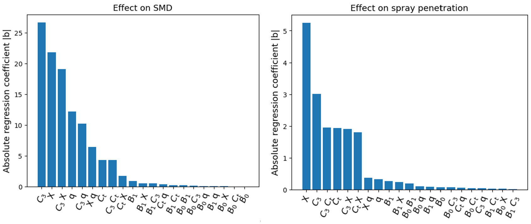
Absolute regression coefficients for the SMD and penetration at 0.8 ms ASOI least squares analysis for the RR + KHRT combination. The higher the bar the more influential the factor.

The most dominant factors selected for the two model combinations were used for a DoE analysis. The other calibration factors were kept constant and equal to the values presented in Table 2. The MATLAB^TM MBC toolbox was used to develop the DoE test plan to be performed via CFD simulations, and also to build a meta-model of the simulation data. The DoE was generated using a 46-point Halton³⁹ sequence. This design was subsequently augmented with a 2² factorial design to place points at the corners of the design space. The augmentation ensured that the responses at the extreme values of the experimental factors were included in the model. The resulting design is illustrated in Figure 8.

Figure 8.

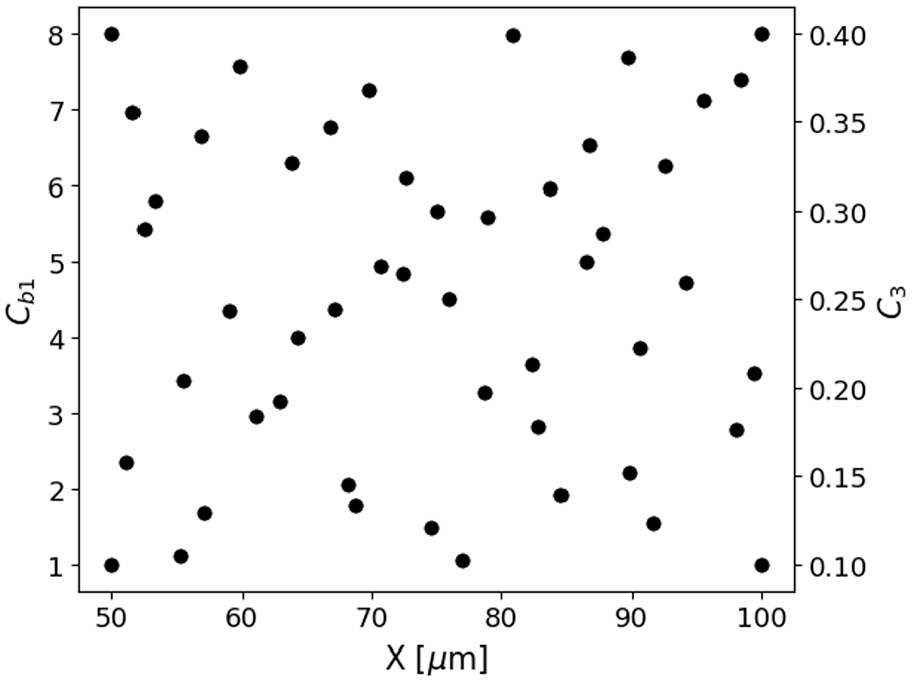
Example response surface design for the simulation meta-model. The design is comprised of a 46-point Halton sequence and augmented with a 2² factorial to place points at the extremes of the experimental region.

The experiment was carried out at 150 and 250 bar injection pressure for both the RR + KHRT and RR + RD combinations. A hybrid RBF-polynomial meta-model^43,44 was used to interpolate the simulation data. Each simulation required about 30 min of computation time on 96 CPUs, implying the total time required for model training was 50 h.

The contour plots of the normalised objective functions for the two model combinations at 150 and 250 bar are presented in Figures 9 and 10, respectively. Both objectives were normalised providing values from 0 – hypothetical perfect match, to 1 – highest error. As shown in Figure 9(a), the combination of the highest X values and C_b₁ in the range of four produces an area of low penetration error. In the same graph, the maximum error is observed for droplet distributions with smaller diameters and the lowest level of break-up threshold. In this case, the spray is formed by relatively small droplets, which show a tendency to disintegrate rapidly. In Figure 8(b) the predicted OBJ2 error was at the minimum level for the whole X range and C_b₁ above 1.8. For this reason, the C_b₁ axis was limited between 1 and 3. The highest error was predicted with the highest X and the lowest C_b₁. It is important to notice how the lowest threshold for bag break-up (C_b₁ factor) produced abnormal simulation responses in terms of both penetration and droplet size distribution. Figure 9(c) and (d) show the modelled objective functions for the RR + KHRT combination at a pressure of 150 bar. In Figure 9(c), OBJ1 has an opposite trend compared to RR + RD, with the highest error predicted for the maximum levels of both X and C₃. An extended low-error zone appears with a value of C₃ lower than 0.2 across all the X range. Similarly to RR + RD, OBJ2 has an extended area of small error with a break-up coefficient above 0.12, as shown in Figure 9(d). Lower C₃ values produce relatively smaller droplet diameters during the spray evolution, unable to replicate the experimental distribution.

Figure 9.

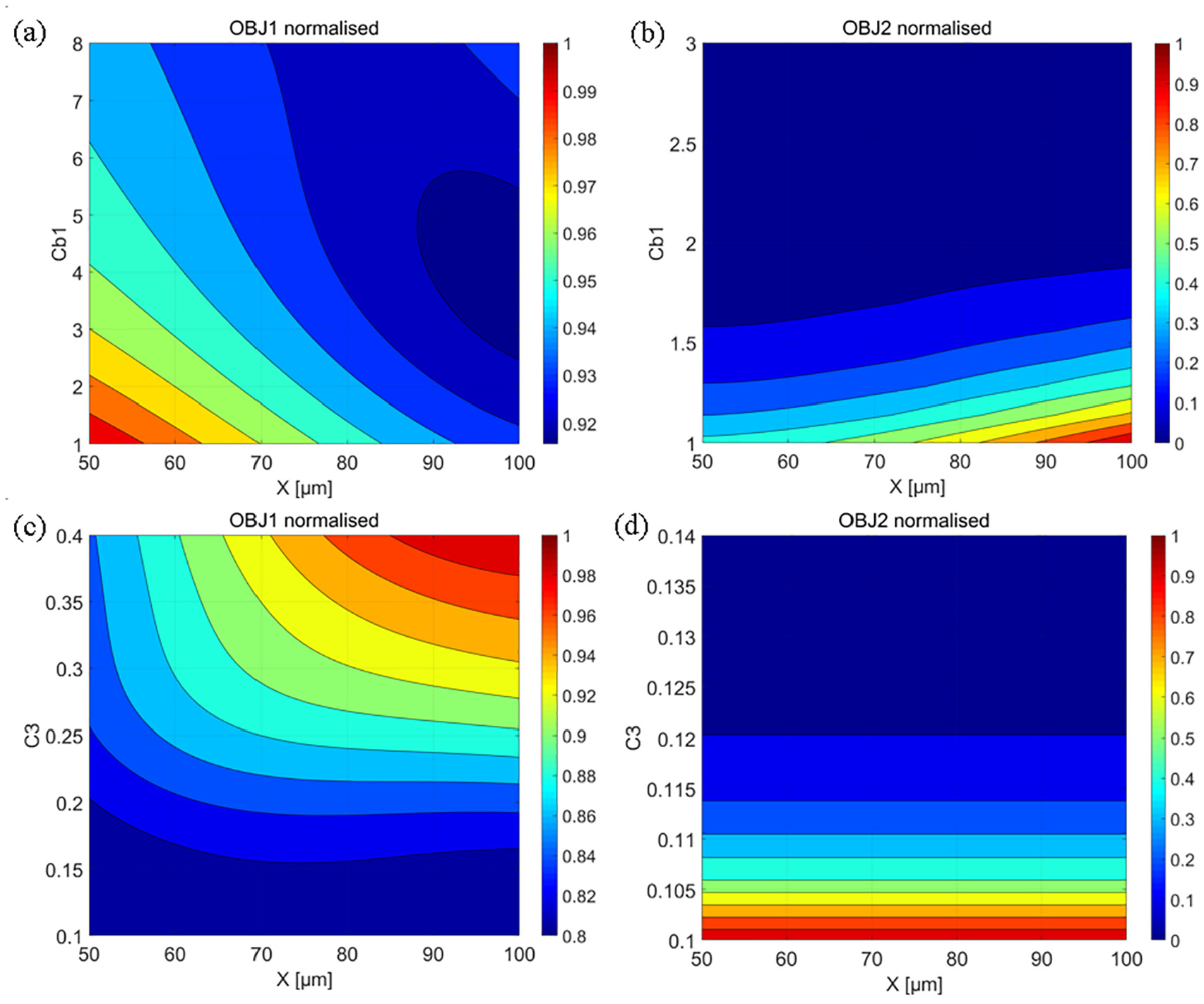
Regression analysis of the objective functions for the two break-up model combinations at 150 bar: (a) RR + RD OBJ1, (b) RR + RD OBJ2, (c) RR + KHRT OBJ1 and (d) RR + KHRT OBJ2.

Figure 10.

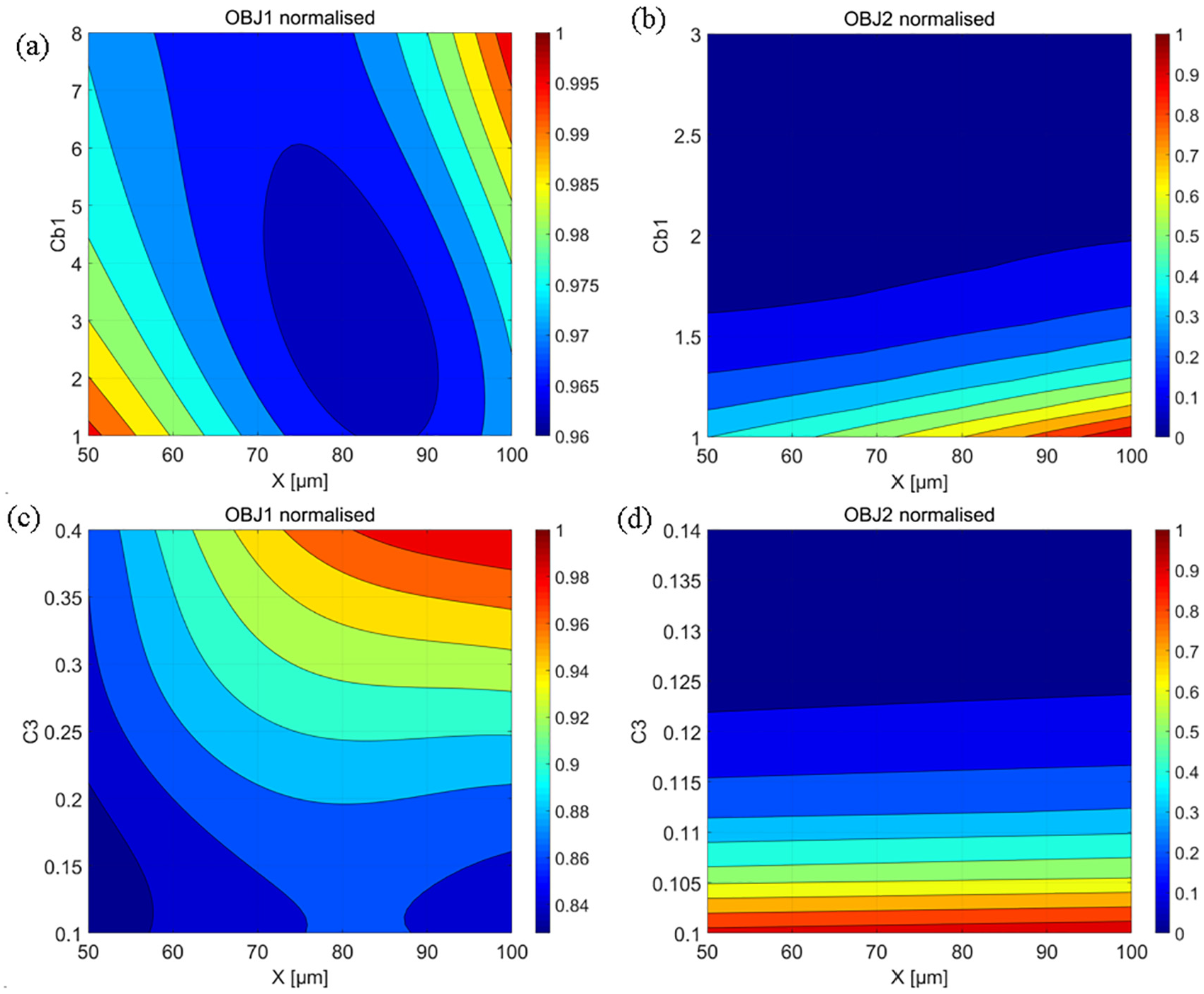
Regression analysis of the objective functions for the two break-up models combinations at 250 bar: (a) RR + RD OBJ1, (b) RR + RD OBJ2, (c) RR + KHRT OBJ1 and (d) RR + KHRT OBJ2.

The increase of injection pressure from 150 to 250 bar produces noticeable variation only for OBJ1 contour plots while OBJ2 is less affected, as shown in Figure 10. In particular, Figure 10(a) introduces two areas of higher penetration error: one at the bottom left corner, similar to the 150 bar case, at small liquid droplet diameters and high-intensity break-up; another at the top right corner where the initial droplet distribution was introduced with the highest value of X and the break-up threshold was at the maximum. In this region, the combination of bigger droplet diameters that persist longer and the increased injection velocity produces an overestimation of the spray penetration. The lower error region is shifted towards a smaller diameter in comparison with the 150 bar case. The effect can be explained with a more atomised distribution needed to reduce the penetration squared error as a consequence of the increased injection pressure. In Figure 10(b), the extended area of low OBJ2 error is similar to the 150 bar case. The area of highest error is also similar and predicted at increasing X with low levels of C_b₁. Figure 10(c) presents two regions of low error, highlighting the possibility of having good prediction performance with different sets of calibration factors. The non-linear nature of the problem emphasises the necessity of an optimisation process. Figure 10(d), proves the strong dependency between OBJ2 and C₃, similarly to the 150 bar case.

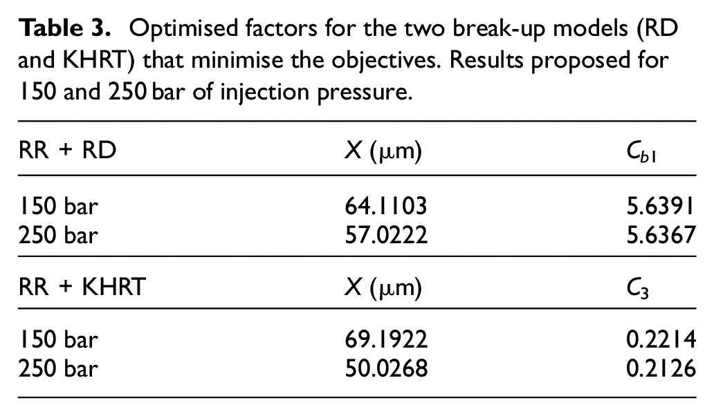
The surrogate models of both objective functions served as an input for the nested optimisation process. Table 3 shows the sets of optimal solutions for all the models’ combinations at the two injection pressures of 150 and 250 bar. The optimisation method found a decreasing trend with injection pressure for E for both model combinations. This is aligned with the physical behaviour of the spray that reduces the diameters of the droplet distribution for higher injection pressure due to the enhanced atomisation.²⁰

Table 3.

Optimised factors for the two break-up models (RD and KHRT) that minimise the objectives. Results proposed for 150 and 250 bar of injection pressure.

RR + RD	X (µm)	C_b ₁
150 bar	64.1103	5.6391
250 bar	57.0222	5.6367
RR + KHRT	X (µm)	C ₃
150 bar	69.1922	0.2214
250 bar	50.0268	0.2126

The modelling results for 150 and 250 bar in terms of spray tip penetration and cumulative size distribution function on a reference plane 50 mm down the injector nozzle, are shown in Figures 11 to 13. The RR + RD combination model in Figure 11 shows an overall satisfactory prediction of spray penetration for both injection pressures investigated. On the contrary, the RR + KH–RT combination model generally over predicts penetration, at least for times beyond 0.25 ms. Both models underestimate the initial part of spray development (up to 0.2 ms), probably due to a combined effect of discharge coefficient error, constant MFR profile adopted for all the nozzles and intrinsic inaccuracy introduced with the numerical code.⁴⁵ In particular, the modelled initial velocity of the droplets was lower in comparison with the experiments even if the reproduced MFR profile matched the opening/closing ramps, the bulk and hence the total mass injected. The error was mitigated for the other injection pressures analysed as shown in the following section. An over prediction is observed in the region of maximum penetration due to a possible higher concentration of liquid in the proximity of the plumes’ tip in comparison with the experiments.⁴⁶ The analysis of the droplet characteristic diameters in Figures 12 and 13 reveals how the RD break-up model was able to capture the experimental quantities with the lowest level of error, showing a reasonable sigmoid shape aligned with the experimental trends. The KH–RT model instead shows an abnormal inflexion around the upper limit of the cumulative distribution. Figure 13 shows the prediction performance in terms of the three characteristic droplet diameters. In particular, SMD is of fundamental importance for the implantation of the spray model within a GDI combustion chamber 3D CFD domain.¹⁰ As above, the RD model performs better, with the KH–RT model grossly overestimating the SMD for both injection pressures. The RR + RD model combination was selected as best to develop a CFD model of the fuel spray analysed.

Figure 11.

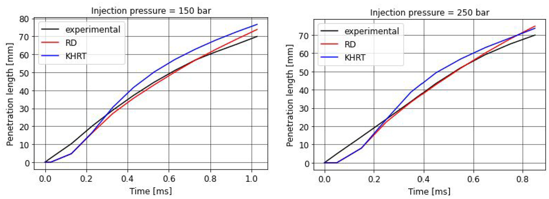
Spray penetration comparison between the two break-up models (RD and KHRT) and the experimental trend at two levels of injection pressure.

Figure 12.

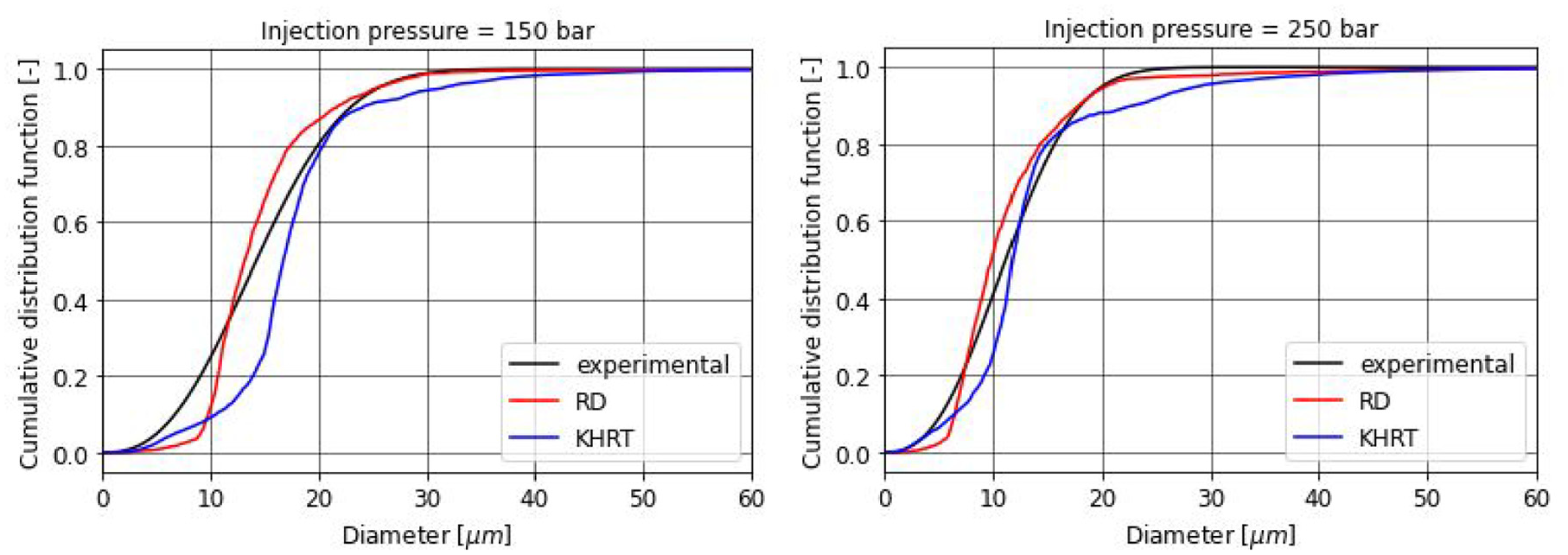
Cumulative distribution function comparison between the two break-up models (RD and KHRT) and the experimental trend at two levels of injection pressure.

Figure 13.

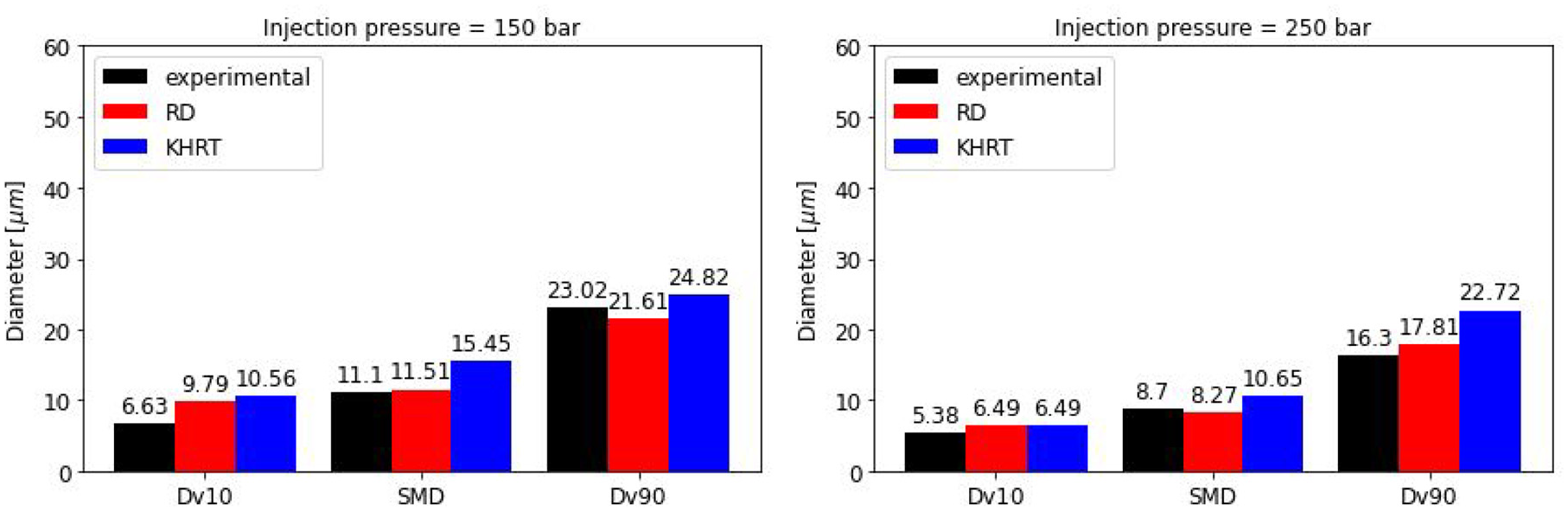
D_v ₁₀, SMD and D_v₉₀ prediction capability of the two break-up models (RD and KH–RT) at two levels of injection pressure. Results obtained on a plane 50 mm down the injector nozzles.

Meta-modelling of spray characteristics

The modelled responses from the DoE analysis in terms of spray tip penetration and SMD are shown in Figure 14 for 150 and 250 bar injection pressure, respectively. The models were obtained with the same methodology introduced with the objective analysis. The correlations between X, C_b₁ and spray characteristics were consistent for both injection pressures. In particular, Figure 14(a) presents the variation of the spray plumes penetration at 0.5 ms ASOI as a function of both calibration factors at 150 bar. As expected, the liquid penetration increases for a droplet size distribution with higher X values and a higher break-up threshold. Across the whole X and C_b₁ space, penetration shows a maximum variation of over 15%, remaining virtually unaffected by levels of C_b₁ lower than two. Figure 14(b) shows the strong dependence between C_b₁ and SMD at 150 bar, a result aligned with the analysis conducted on OBJ2 (see Figure 9(b)). Importantly, the size of the liquid droplets can be tuned to a specific SMD modifying the break-up coefficient, almost independently of the initial size distribution X. The SMD tripled in the range of calibration constants analysed. Figure 15 and b extend the analysis to the 250 bar injection pressure. The dependencies are largely similar to the 150 bar case; in particular, Figure 15 shows that the spray penetration reaches a minimum for X in the range 75–100 and C_b₁ lower than two. The maximum penetration variation was 11% and hence aligned with the previous case. Consistently with the lower injection pressure, the region of highest penetration is predicted for the highest values of both X and C_b₁. In terms of SMD variation (Figure 14(d)), the maximum SMD level is reduced by 60% in comparison with the 150 bar case (13–8 µm). The variation of calibration factors in the range proposed can produce a quadrupling SMD value.

Figure 14.

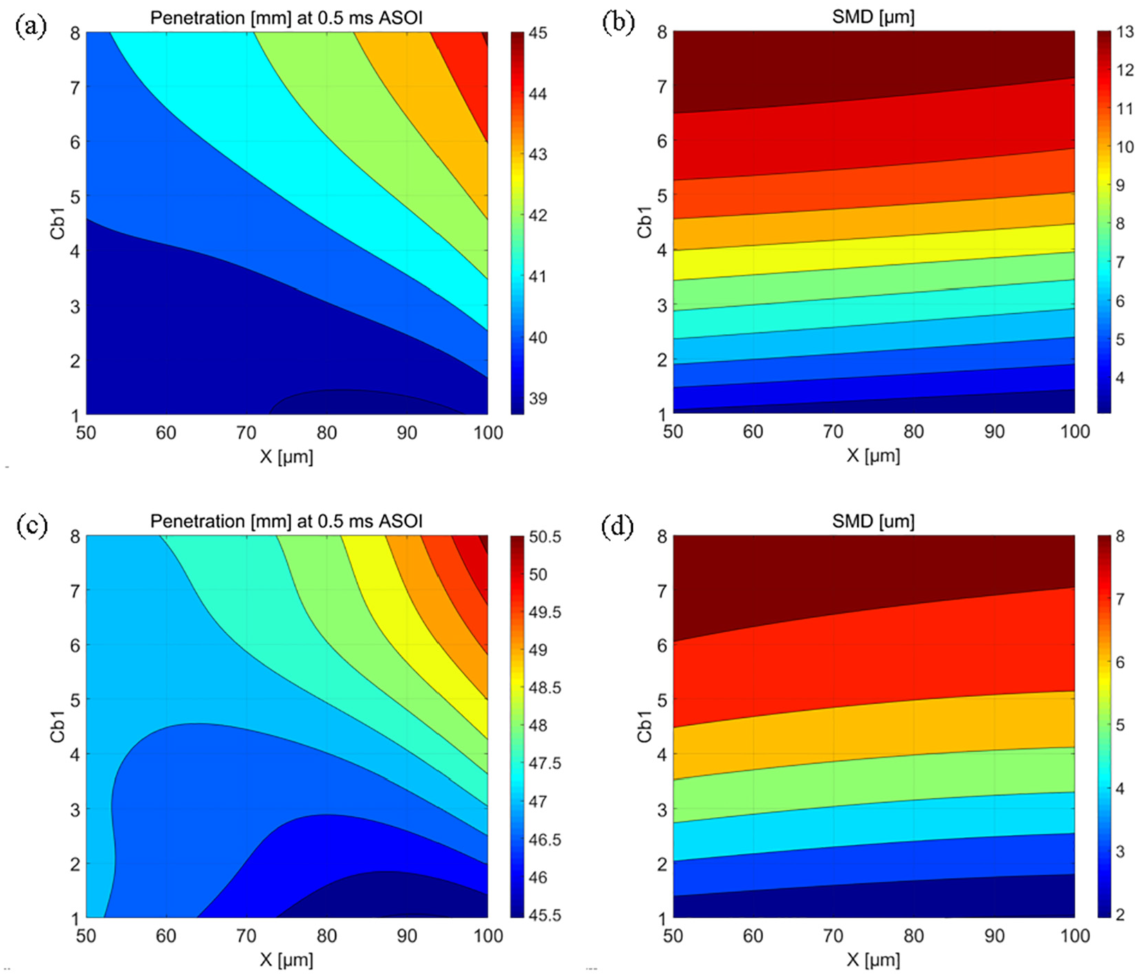
Contour plots of spray characteristics as a function of relevant calibration constants: (a) spray penetration at 0.5 ms ASOI and (b) SMD at 50 mm down the injector at 150 bar; (c) spray penetration at 0.5 ms ASOI and (d) SMD at 50 mm down the injector at 250 bar.

Figure 15.

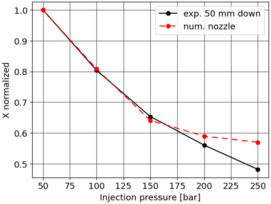
Normalised X as a function of injection pressure. The experimental quantity is reconstructed based on the SMD available on a reference plane 50 mm down the injector. The numerical quantities are the values imposed at the nozzle exit within the 3D domain.

Calibration methodology extended to other injection pressures

The methodology proposed was extended to 50, 100 and 200 bar injection pressure. Figure 15 shows how the E variation as a function of injection pressure follows the corresponding quantity reconstructed from experimental SMD data taken 50 mm down the injector nozzle. Within the limitations of the available experimental data, the optimal solutions obtained through the proposed methodology were able to capture the physical behaviour of the spray process.

Penetration, cumulative size distribution and characteristic diameters results are shown in Figure 16. Figure 16(a) to (c) show good accuracy of liquid penetration in comparison with the experimental data. At 50 bar injection pressure, the penetration is well predicted, with a slight under prediction on the ballistic region of the spray. The 100 bar case reveals a slight underestimation of the liquid penetration in the same region, whereas an almost perfect match is obtained from 50 mm up to the limit of the measurement window (70 mm). On the contrary, the 200 bar case exhibits a good prediction up to 50 mm and a general overestimation up to 70 mm. The sigmoid shape of the cumulative distribution function is presented in Figure 16(d) to (f). The cumulative function of the 50 bar case presents a good prediction up to the SMD (32% of the distribution) and an underestimation of the predicted diameters above 40% of the distribution, for droplet size between 20 and 40 µm. This behaviour is highlighted in Figure 16(g), where the numerical D_v₉₀ was 38% smaller in comparison with the experimental counterpart. A potential reason for this mismatch is a more severe variation of the experimental droplet distribution at the lower injection pressures and this is reflected in the experimental D_v₉₀ between 100 and 50 bar. In contrast, both SMD and D_v₁₀ followed a smooth evolution as the injection pressure varies. The model produced smaller droplets due to the lowest break-up coefficient obtained through the optimisation process. Since SMD, D_v₁₀ and penetration are well predicted and the break-up coefficient follows a linear trend with the injection pressure, the tuning of the coefficient is considered sufficient for an accurate spray model calibration. The 100 bar and the 200 bar cases, presented in Figure 16(e) and (h) and in Figure 16(f) and (i), respectively, show similar behaviour but improved accuracy as the injection pressure increases.

Figure 16.

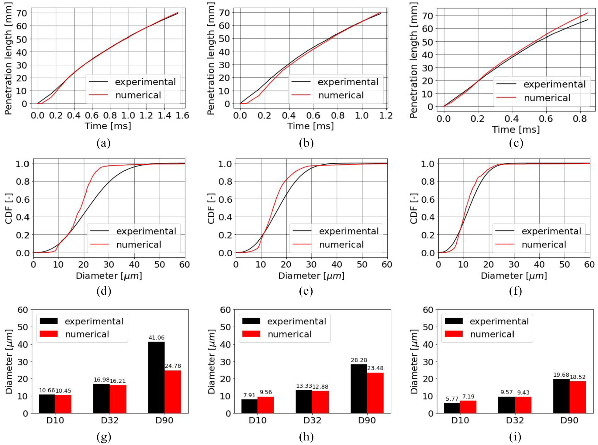
Prediction performance of the calibrated fuel spray in terms of penetration at: (a) 50, (b) 100 and (c) 200 bar; in terms of cumulative distribution function (CDF) 50 mm down the injector location at (d) 50, (e) 100 and (f) 200 bar; and in terms of D_v₁₀, SMD and D_v₉₀ at (g) 50, (h) 100 and (i) 200 bar.

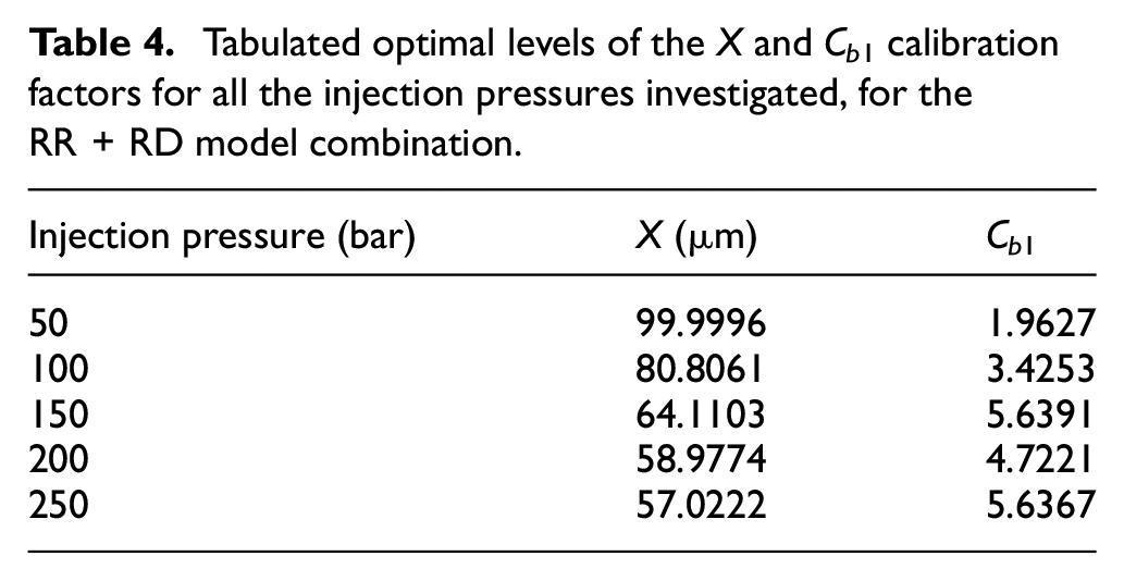
The optimised calibration factors X and C_b₁ for all the injection pressures investigated are reported in Figure 17 and Table 4. The other factors (q, C_b₂, C_s₁ and C_s₂) were kept constant and equal to the typical values presented in Table 2. The reduction of X with increasing injection pressure is consistent with the expected physical behaviour – a reduction of droplet diameter due to a more intense atomisation process.²⁰ The latter is stronger up to 150 bar, to then reduce between 150 and 250 bar, possibly due to the physical limitation of the fixed-geometry injector. Factor C_b1 increases almost linearly between 50 and 150 bar, most likely to compensate for the effect of velocity on droplet disintegration. Between 150 and 250 bar C_b₁ tends to remain stable, although the optimisation process at 200 bar returns an unexpected slight reduction. This remains unexplained at this stage and will be the object of further investigation in the near future.

Figure 17.

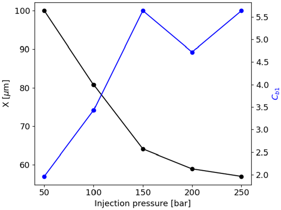
Optimal levels of the X and C_b₁ calibration factors as functions of injection pressure, for the RR + RD model combination.

Table 4.

Tabulated optimal levels of the X and C_b₁ calibration factors for all the injection pressures investigated, for the RR + RD model combination.

Injection pressure (bar)	X (µm)	C_b ₁
50	99.9996	1.9627
100	80.8061	3.4253
150	64.1103	5.6391
200	58.9774	4.7221
250	57.0222	5.6367

Spray morphology analysis

A double view-point morphology comparison between experimental (liquid and vapour) and numerical (liquid) spray images is shown in Figure 18. Only one injection pressure – 250 bar, at 0.8 ms ASOI to have a well extended spray, is presented for brevity. For the numerical images, each plume is distinguished by a different colour and the droplets are plotted by dimension. The numerical results are generally in good agreement with experimental plumes’ shape, overall cone angle and tips’ penetration. The images show a more jagged shape of the experimental plumes compared to the smoothness of the numerical ones, likely to be due to the subtle threshold between liquid and vapour phase.^15,46–48 Moreover, the RANS numerical approach simplifies the smallest turbulent scales, adding another potential source of difference.⁴⁹ However, the trade-off between computational costs and accuracy was considered acceptable. Regions of the spray rich in fuel vapour were reproduced with small droplets as evidence of a strong evaporation rate. The wide hole configuration of the injector produced generally recognisable structures for each of the five plumes. From the droplet dimension analysis, four distinguished regions can be observed:

Near-field: The typical liquid ligaments at the nozzle exit^50,51 are simplified by imposing an atomised spray formed by clusters of big droplets with a maximum diameter D_d = 100 µm. Smaller droplets also exist in this region, as evidenced by a SMD_initial of 26.5 µm obtained imposing the calibrated constant factors. These small droplets reproduce the rapid phase-change of the fuel droplets and consequently the primary atomisation mechanism.

Plume bulk: The secondary break-up due to pressure instability and shearing process^15,34,51 produce a large variety of diameters with evidence of big droplets that tend to persist in the proximity of the central region of the plumes. As explained in the next paragraph, several droplets in this region show a stagnation behaviour, that is, almost zero momentum.

Plume interface: The air entrainment and generally the interaction between the gas-liquid phases promotes rapid evaporation of the fuel. Turbulent phenomena were noticeable experimentally and fish-bone structures were evident for the most external plumes. The behaviour was reproduced with a scattered distribution of small droplets showing evidence of a strong evaporation rate.^51,52

Plume tip: This region is usually characterised by a higher concentration of fuel vapour and a fully developed secondary break-up.⁴⁶ The clusters of highly disintegrated droplets (D_d < 10 µm) mimic the combined effect of turbulent motion and drag force, as well as the longest residence time (0.8 ms) of the liquid injected.

Figure 18.

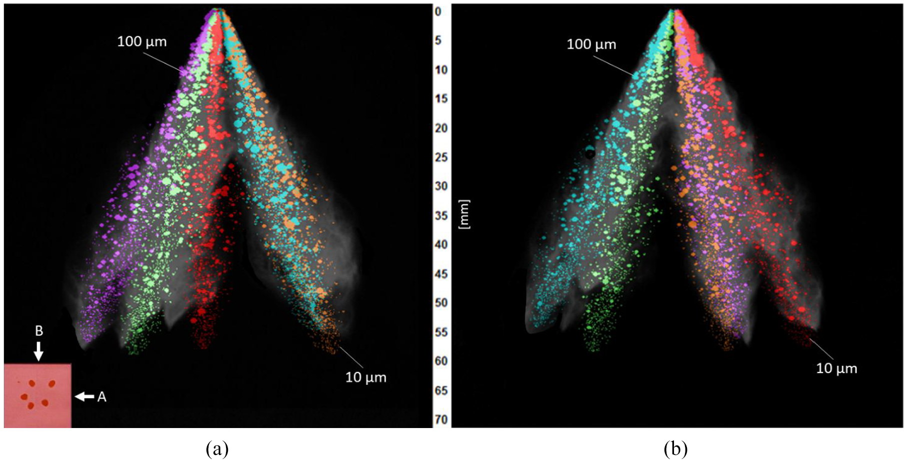
Morphology comparison between experimental (grey) and numerical (coloured) results. The images were captured at 250 bar injection pressure and 0.8 ms ASOI. A and B represent the two viewpoints available from the experiments. The small image in the bottom left corner shows the spray’s footprint obtained experimentally at 50 mm down the nozzle, at an injection pressure of 35 bar.

Figure 19 presents the almost linear correlation between the computed mid-range velocity magnitude and SMD. Each point in the graph represents an injection pressure, from 50 to 250 bar. The velocity magnitude was evaluated from instantaneous quantities as an average between maximum and minimum velocity. The investigated range of pressures reveals a variation of SMD and velocity magnitude of −50% and 113%, respectively. Considering each of the 50 bar increments, the maximum velocity gain and SMD reduction were obtained between 50 and 100 bar. In the range 200–250 bar both velocity and SMD variation were marginal in comparison with other increments. The phenomenon is of fundamental interest to define a trade-off between droplet velocity and dimension necessary to design injection strategies for emission reduction.⁵³ On one hand, in a given cylinder geometry, the increase of spray velocity might yield a more intense spray impact on the piston crown with consequent liquid film deposit. On the other hand, a well atomised spray is necessary to speed-up the air-fuel mixing process.^34,53,54 Figure 19 also shows the computed spray images with droplets plotted by instantaneous velocity. The maximum velocity of the droplets is reached soon after the nozzle exit and then decrease rapidly after around 15 mm. The velocity deteriorates along each plume with the lowest velocity in the proximity of the plumes’ tips. For all the pressures, stagnation is evident in the plumes’ bulk region; this behaviour might be due to a combined effect of air recirculation and drag forces.

Figure 19.

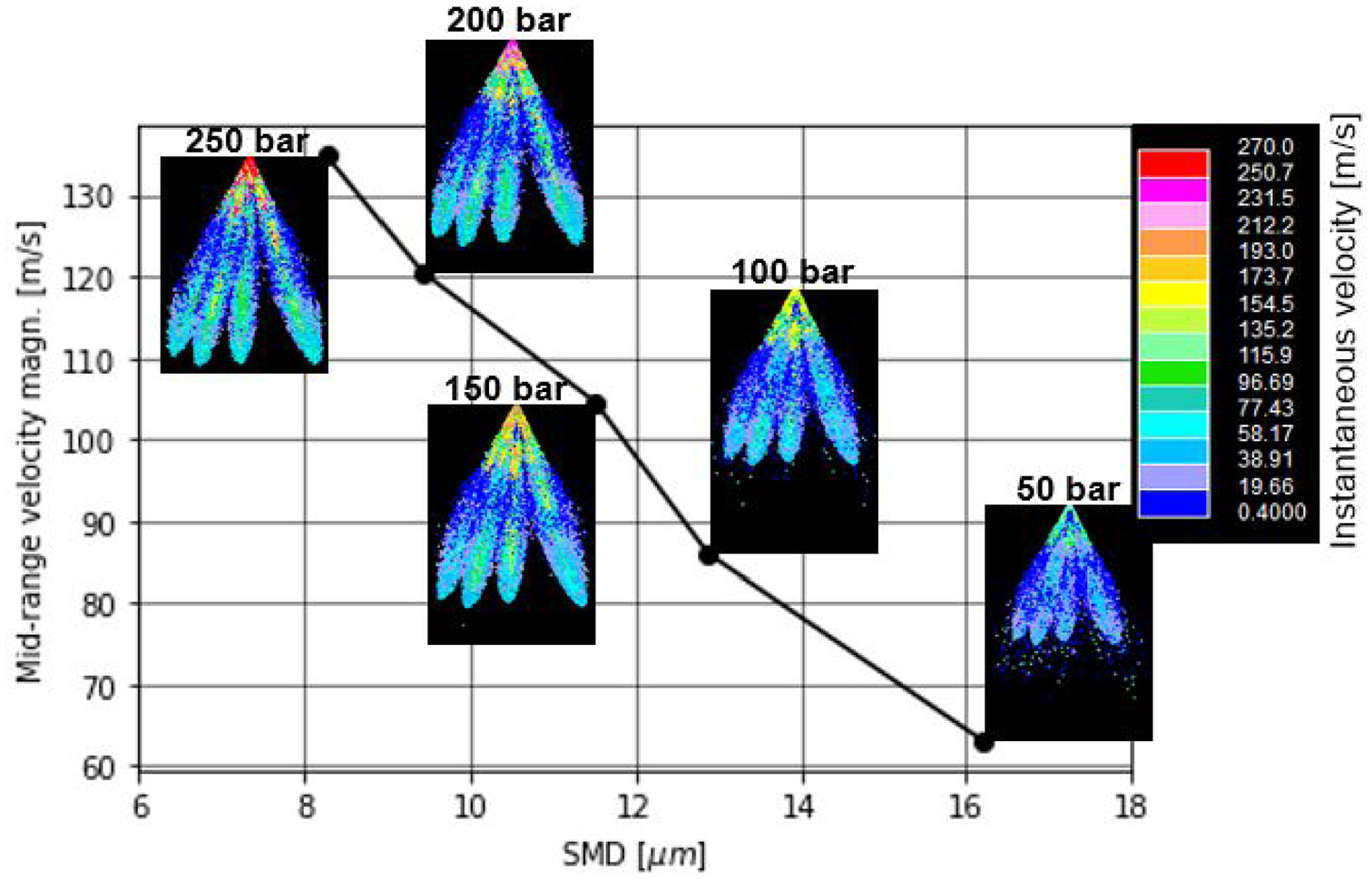
Predicted values of SMD as a function of the velocity magnitude for every injection pressure investigated. Snapshots were done at 0.8 ms ASOI.

Conclusions

A CFD model of high-pressure fuel injections was developed to accurately predict fundamental spray characteristics over a wide range of operating conditions. The two most commonly used break-up models, KHRT and RD, were studied in terms of prediction performance in combination with a RR mono-modal initial droplet size distribution. To minimise the number of calibration factors, a half factorial screening design was used for each model combination, yielding the factors that showed a dominant effect on spray penetration and SMD. A subsequent space-filling DoE design produced a testing space for the selected factors and served as input for the 3D CFD simulations. The results were used to produce surrogate models in terms of objective functions that, in turn, were minimised following a nested optimisation procedure. An optimal set of calibration factors was defined for each of the two model combinations. The analysis of the prediction performance revealed that RR + RD outperforms RR + KHRT.

The following main outcomes can be drawn from the investigation:

The proposed statistical and optimisation methodology was able to first identify and then produce optimal levels of the dominant spray model calibration factors that enable good prediction of high-pressure spray behaviour in terms of tip penetration, droplet size distribution and morphology.

Importantly, the proposed methodology can be extended to other physical mechanisms and their descriptive phenomenological models to reveal how the relevant calibration factors may influence the model responses over wide ranges of operating conditions.

The half-factorial screening highlighted how reasonable prediction of experimental spray characteristics can be obtained by tuning only the initial RR distribution parameter X and one break-up factor that is responsible for the secondary atomisation process. The dominant break-up factors were C_b₁ and C₃ for the RR + RD and the RR + KHRT, respectively.

RR+RD was the best model combination to predict all the main characteristics of a high-pressure fuel spray between 50 and 250 bar, with the optimisation of only two calibration factors. RR + KHRT overestimated both spray penetration and droplet size distribution for 150 and 250 bar injection pressure. Therefore, the latter model combination requires a more refined and computationally heavier calibration procedure to equal the performance of RR + RD.

The optimised calibration factors revealed how X and the break-up coefficient C_b1 can be assumed to be directly and inversely proportional to the injection pressure, respectively. The break-up coefficient increases to compensate for the effect of an enhanced droplet disintegration with a higher velocity induced by higher injection pressure.

With a detailed regression analysis, it was possible to create contour plots of calibration factors and spray characteristics (penetration at 0.5 ms ASOI and SMD) that can facilitate the initial stage of model calibration and to evaluate the order of magnitude of quantities involved. As X increases in the range 50–100 µm and C_b₁ in the range 1–8, penetration increases by more than 10% while SMD triples and quadruples for 150 and 250 bar, respectively.

The experimental ligaments in the proximity of the injector nozzle were simplified with a droplet size distribution composed of relatively large and fast droplets that quickly disintegrate along the plume. Typical fishbone structures, at the interface of the plumes, were reproduced with highly atomised clusters of droplets.

An almost linear correlation exists between the computed average droplets velocity magnitude and SMD. This is of fundamental interest to aid in the development of engine injection strategies that aim to both maximise air-fuel mixing and reduce liquid film deposition.

Footnotes

Acknowledgements

The authors would like to acknowledge Ford Motor Company and Siemens Digital Industries Software for the support provided.

Declaration of conflicting interests

The author(s) declared no potential conflicts of interest with respect to the research, authorship, and/or publication of this article.

Funding

The author(s) disclosed receipt of the following financial support for the research, authorship, and/or publication of this article: This investigation was financially supported by the Advanced Propulsion Centre (APC), as part of the Ford-led APC6 DYNAMO project, TSB/APC Project Ref. 113130.

ORCID iDs

Davide Domenico Sciortino

Fabrizio Bonatesta

References

Sementa

Maria Vaglieco

Catapano

Thermodynamic and optical characterizations of a high performance GDI engine operating in homogeneous and stratified charge mixture conditions fueled with gasoline and bio-ethanol. Fuel 2012; 96: 204–219.

Bonatesta

Altamore

Kalsi

Cary

. Fuel economy analysis of part-load variable camshaft timing strategies in two modern small-capacity spark ignition engines. Appl Energy 2016; 164: 475–491.

Liu

S-H

Lin

K-Y

B-Z

Song

Gong

. Experimental study on the stratified and homogeneous charge of a direct-injection spark ignition methanol engine. Proc IMechE, Part D: J Automobile Engineering 2011; 225: 236–245.

Singh

Han

Fatouraie

Mansfield

Wooldridge

Boehman

. Influence of fuel injection strategies on efficiency and particulate emissions of gasoline and ethanol blends in a turbocharged multi-cylinder direct injection engine. Int J Engine Res 2021; 22(1): 152–164.

Leach

Stone

Richardson

, et al. Particulate emissions from a highly boosted gasoline direct injection engine. Int J Engine Res 2018; 19(3): 347–359.

Stadler

Brunner

Wachtmeister

Sauerland

. Experimental investigations on high pressure gasoline injection up to 800 bar for different combustion modes. MTZ Worldw 2019; 80: 52–57.

Gasoline Direct Injection (GDI). System market size by component (electronic control units, fuel injectors, fuel pumps, sensors), by application (passenger Car [PC], commercial vehicle [CV]), Industry analysis report, regional outlook, growth potential, competitive market share & forecast, 2016 – 2024. Selbyville, DE: Global Market Insights Inc. 2017.

Sciortino

Bonatesta

Hopkins

Yang

Morrey

. A combined experimental and computational fluid dynamics investigation of particulate matter emissions from a wall-guided gasoline direct injection engine. Energies 2017; 10: 1408.

Bonatesta

Chiappetta

La Rocca

. Part-load particulate matter from a GDI engine and the connection with combustion characteristics. Appl Energy 2014; 124: 366–376.

10.

Biagiotti

Bonatesta

Tajdaran

, et al. Modelling liquid film in modern GDI engines and the impact on particulate matter emissions – part 1. Int J Engine Res 2021; pp 1–24. DOI: 10.1177/14680874211024476.

11.

Bokor

Rohani

Humphries

Morrey

Bonatesta

. Investigating the impact of gasoline composition on PN in GDI engines using an improved measurement method. Int J Engine Res 2020; 1468087420970374.

12.

Chambliss

Silva

West

Zeinali

Minjares

. Estimating source-attributable health impacts of ambient fine particulate matter exposure: global premature mortality from surface transportation emissions in 2005. Environ Res Lett 2014; 9(10): 4009.

13.

Köpple

Jochmann

Kufferath

Bargende

. Investigation of the parameters influencing the spray-wall interaction in a GDI engine – prerequisite for the prediction of particulate emissions by numerical simulation. SAE Int J Engines 2013; 6: 911–925.

14.

Lucchini

D’Errico

Onorati

Bonandrini

Venturoli

Di Gioia

. Development and application of a computational fluid dynamics methodology to predict fuel–air mixing and sources of soot formation in gasoline direct injection engines. Int J Engine Res 2014; 15(5): 581–596.

15.

Migliaccio

Montanaro

Lucchini

Allocca

Paredi

. Numerical investigation on GDI spray under high injection pressure up to 100 MPa. SAE technical paper0148-7191, 2020.

16.

Price

Hamzehloo

Aleiferis

Richardson

. Numerical modelling of fuel spray formation and collapse from multi-hole injectors under flash-boiling conditions. Fuel 2018; 221: 518–541.

17.

The Automotive Council. Automotive technology roadmap, https://www.automotivecouncil.co.uk/2013/09/automotive-technology-roadmaps/ (2013).

18.

Wang

Zhao

. Numerical simulation of the gasoline spray with an outward-opening piezoelectric injector: a comparative study of different breakup models. SAE technical paper 2018-01-0272, 2018.

19.

Braga

Vaz

de Moraes Martins

Hindi

Huebner

. 3D numerical characterization of a multi-holes injector in a quiescent vessel and its application in a single-cylinder research engine using ethanol. SAE technical paper 0148-7191, 2017.

20.

Teng

. A model-based analysis on size distribution and rate of evaporation for fuel drops in a gasoline spray in the engine. SAE technical paper0148-7191, 2012.

21.

Costa

Sorge

Allocca

. CFD optimization for GDI spray model tuning and enhancement of engine performance. Adv Eng Softw 2012; 49: 43–53.

22.

Perini

Reitz

. Improved atomization, collision and sub-grid scale momentum coupling models for transient vaporizing engine sprays. Int J Multiphase Flow 2016; 79: 107–123.

23.

Taghavifar

Anvari

Mousavi

. Assessment of varying primary/secondary breakup mechanism of diesel spray on performance characteristics of HSDI engine. Fuel 2020; 262: 116622.

24.

Khan

Hélie

Gorokhovski

Sheikh

. Experimental and numerical study of flash boiling in gasoline direct injection sprays. Appl Therm Eng 2017; 123: 377–389.

25.

Hung

DLS

Harrington

Gandhi

, et al. Gasoline fuel injector spray measurement and characterization – a new SAE J2715 recommended practice. SAE Int J Fuel Lubricants 2008; 1: 534–548.

26.

Abani

Bakshi

Ravikrishna

. Multi-dimensional modelling of spray, in-cylinder air motion and fuel-air mixing in a direct-injection engine. Sadhana 2007; 32(5): 597–617.

27.

Paredi

Lucchini

D’Errico

Onorati

Pickett

Lacey

. Validation of a comprehensive computational fluid dynamics methodology to predict the direct injection process of gasoline sprays using spray G experimental data. Int J Engine Res 2020; 21(1): 199–216.

28.

Star-CD methodology manual. Version 4.32 ed. Computational Dynamics Limited, Siemens, London.

29.

Stiesch

Modeling engine spray and combustion processes. Springer Science & Business Media, Berlin Heidelberg: Springer-Verlag, 2003.

30.

Cavicchi

Postrioti

Giovannoni

Fontanesi

Bonandrini

Di Gioia

. Numerical and experimental analysis of the spray momentum flux measuring on a GDI injector. Fuel 2017; 206: 614–627.

31.

Befrui

D’Onofrio

. Primary atomization of a GDi multi-hole plume using VOF-LES method. SAE technical paper 2014-01-1125, 2014.

32.

Lefebvre

McDonell

. Atomization and sprays. Boca Raton, FL: CRC press, 2017.

33.

Reitz

Beale

. Modeling spray atomization with the Kelvin-Helmholtz/Rayleigh-Taylor hybrid model. Atomization Sprays 1999; 9: 623–650.

34.

Reitz

Diwakar

. Effect of drop breakup on fuel sprays. SAE Trans 1986; 1986: 218–227.

35.

Patterson

Reitz

. Modeling the effects of fuel spray characteristics on diesel engine combustion and emission. SAE Trans 1998; 1998: 27–43.

36.

Montgomery

. Design and analysis of experiments. 8th ed. Hoboken, NJ: John Wiley & Sons, 2013.

37.

Box

GEP

Meyer

. An analysis for unreplicated fractional factorials. Technometrics 1986; 28: 11–18.

38.

Ryberg

A-B

Domeij Bäckryd

Nilsson

. Metamodel-based multidisciplinary design optimization for automotive applications. Linköping: Linköping University Electronic Press, 2012.

39.

Halton

. Algorithm 247: radical-inverse quasi-random point sequence. Commun ACM 1964; 7: 701–702.

40.

Stein

. Large sample properties of simulations using Latin hypercube sampling. Technometrics 1987; 29: 143–151.

41.

Sobol’

. On the distribution of points in a cube and the approximate evaluation of integrals. Zhurnal Vychislitel’noi Matematiki i Matematicheskoi Fiziki 1967; 7: 86–112.

42.

Niederreiter

. Constructions of (t, m, s)-nets and (t, s)-sequences. Finite Fields Appl 2005; 11: 578–600.

43.

Lazzaro

Montefusco

. Radial basis functions for the multivariate interpolation of large scattered data sets. J Comput Appl Math 2002; 140: 521–536.

44.

Škala

. A practical use of radial basis functions interpolation and approximation. Investigación Operacional 2016; 37: 137–145.

45.

Mohapatra

Schmidt

Sforozo

, et al. Collaborative investigation of the internal flow and near-nozzle flow of an eight-hole gasoline injector (engine combustion network spray G). Int J Engine Res 2020; 2020: 1468087420918449.

46.

Paredi

Lucchini

D’Errico

, et al. CFD modeling of spray evolution for spark-ignition, direct injection engines. In: AIP Conference Proceedings, Vol. 2191, No. 1, Dec 17 2019, p.020125. AIP Publishing LLC.

47.

Roque

Foucher

Lamiel

Imoehl

Lamarque

Helie

. Impact of gasoline direct injection fuel films on exhaust soot production in a model experiment. Int J Engine Res 2020; 21: 367–390.

48.

Allocca

Bartolucci

Cordiner

, et al. ECN Spray G injector: assessment of numerical modeling accuracy. SAE technical paper0148-7191, 2018.

49.

Valentino

Jiang

Zhao

. A comparative rans/les study of transient gas jets and sprays under diesel conditions. Atomization Sprays 2007; 17: 451–472.

50.

Lasheras

Villermaux

Hopfinger

. Break-up and atomization of a round water jet by a high-speed annular air jet. J Fluid Mech 1998; 357: 351–379.

51.

Reitz

Diwakar

. Structure of high-pressure fuel sprays. SAE technical paper 870598, 1987.

52.

Hori

Senda

Kuge

Fujimoto

. Large eddy simulation of non-evaporative and evaporative diesel spray in constant volume vessel by use of KIVALES. SAE technical paper 2006-01-3334, 2006.

53.

Zhao

F-Q

Lai

M-C

Harrington

. A review of mixture preparation and combustion control strategies for spark-ignited direct-injection gasoline engines. SAE technical paper 970627, 1997.

54.

Reitz

Ogawa

Payri

, et al. IJER editorial: the future of the internal combustion engine. Int J Engine Res 2020; 21: 3–10.

A systematic approach to calibrate spray and break-up models for the simulation of high-pressure fuel injections

Abstract

Keywords

Introduction

Methodology

Experimental setup for spray data acquisition

Model description and implementation

Models selection and calibration

Factor screening process

Response surface design and modelling

Definition of response metrics and optimisation process

Results and discussions

Factorial screening and spray model selection

Meta-modelling of spray characteristics

Calibration methodology extended to other injection pressures

Spray morphology analysis

Conclusions

Footnotes

Acknowledgements

Declaration of conflicting interests

Funding

ORCID iDs

References