
Abstract
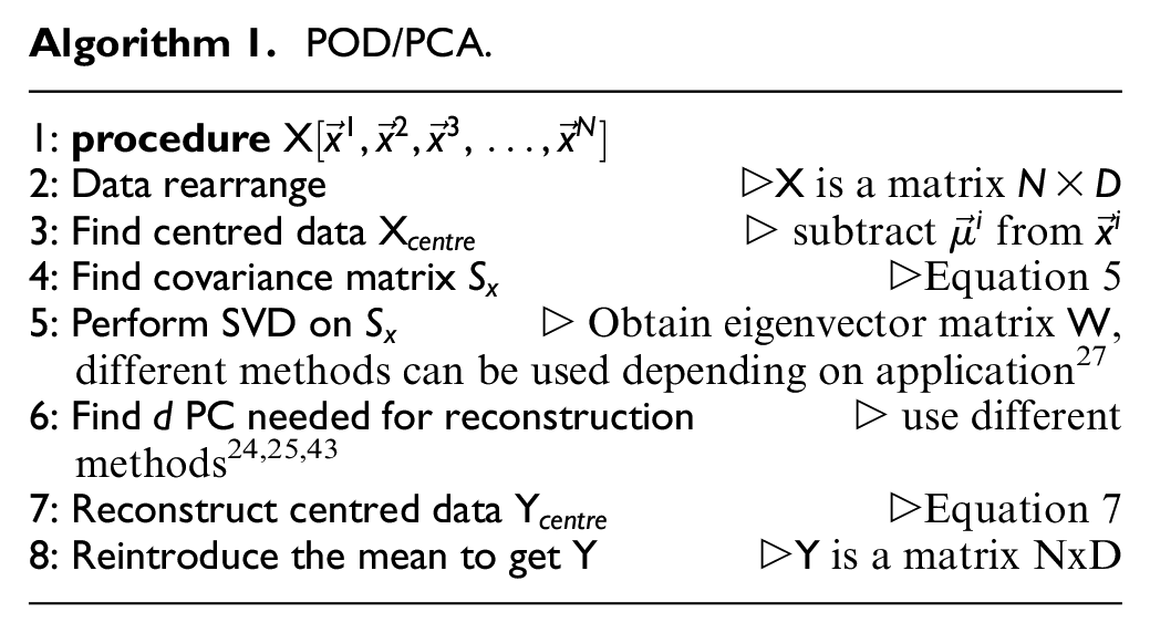
In this article, different manifold reduction techniques are implemented for the post-processing of Particle Image Velocimetry (PIV) images from a Spark Ignition Direct Injection (SIDI) engine. The methods are proposed to help make a more objective comparison between Reynolds-averaged Navier-Stokes (RANS) simulations and PIV experiments when Cycle-to-Cycle Variations (CCV) are present in the flow field. The two different methods used here are based on Singular Value Decomposition (SVD) principles where Proper Orthogonal Decomposition (POD) and Kernel Principal Component Analysis (KPCA) are used for representing linear and non-linear manifold reduction techniques. To the authors’ best knowledge, this is the first time a non-linear manifold reduction technique, such as KPCA, has ever been used in the study of in-cylinder flow fields. Both qualitative and quantitative studies are given to show the capability of each method in validating the simulation and incorporating CCV for each engine cycle. Traditional Relevance Index (RI) and two other previously developed novel indexes: the Weighted Relevance Index (WRI) and the Weighted Magnitude Index (WMI), are used for the quantitative study. The results indicate that both POD and KPCA show improvements in capturing the main flow field features compared to ensemble-averaged PIV experimental data and single cycle experimental flow fields while capturing CCV. Both methods present similar quantitative accuracy when using the three indexes. However, challenges were highlighted in the POD method for the selection of the number of POD modes needed for a representative reconstruction. When the flow field region presents a Gaussian distribution, the KPCA method is seen to provide a more objective numerical process as the reconstructed flow field will see convergence with an increasing number of modes due to its usage of Gaussian properties. No additional criterion is needed to determine how to reconstruct the main flow field feature. Using KPCA can, therefore, reduce the amount of analysis needed in the process of extracting the main flow field while incorporating CCV.
Keywords
Introduction
The in-cylinder air motion strongly influences the homogeneity of the air-fuel mixture, and thus the combustion and emissions characteristics of spark ignition direct injection (SIDI) engines.1–3 The development of high-speed particle image velocimetry (PIV) enables crank angle-resolved in-cylinder flow measurement for a few hundred consecutive cycles with a high spatial resolution (usually millimetre in scale).4,5 With increasing computational power, various numerical techniques have been developed to simulate in-cylinder flow data with reasonably high fidelity. However, due to the demand of shortening the complex engine design process for industrial use, the availability of statistically converged full cycle high-fidelity simulations such as large eddy simulation (LES) and direct numerical simulation (DNS) are still mostly constrained to research facilities. The most commonly used turbulence modelling tools for industrial engine development are still based on Reynolds-averaged Navier-Stokes (RANS) approach. Although provided as a good predictive tool for global characteristics, it is well known to the modelling community that RANS-based models are unable to capture the stochastic nature of the turbulent flow. Significant progress has been made over the years in RANS models to include the unsteady behaviour of turbulent flows. These techniques vary from adding additional unsteady terms 6 to renormalised Navier Stokes equations 7 where small scale perturbations can be included. With both advancements in experimental techniques and numerical methods, the question arises: is it accurate to compare converged experimental ensemble-averaged quantities directly with those from RANS-based models, especially when flow fields present cycle-to-cycle variations (CCV)?
Yang et al. 8 performed a comparative engine cold flow analysis between the RANS flow field and cycle-averaged LES simulation using the PIV ensemble average field as the reference data. RANS simulations were found to predict reasonably good qualitative trends for the mean flow and turbulence, but less accurate descriptions of the mean flow structures and turbulence distribution are found when compared with ensemble-averaged LES and PIV. Earlier studies from Wu et al. 9 used RANS-based combustion models to predict OH radical fields of a combusting non-premixed methane jet. A poor agreement was found between the predicted RANS OH radical, and the converged experimental ensemble average. A higher degree of similarity is, however, seen between the results of the RANS simulation and some of the single shot OH-PLIF images than the similarity between the simulations and the ensemble-averaged OH-PLIF results. From a simulation point of view, one would expect a Reynolds averaged field to have a fairly gradual rise in temperature over a broad area of the flow. However, further statistical analysis suggested that the mean convective velocity term contributes to a rapid rise in the temperature terms, whereas an ensemble-averaged field from the experiment is smoothed both in time and space. The study also suggested that more than 100 realizations of LES would be necessary to enable the comparison with the experimental ensemble-averaged results. Studies have also been carried out by Stein et al. 10 comparing LES simulations of in-nozzle flow in turbulent opposed jets with PIV experiments. With a novel statistical method, a comparison of metrics derived from individual cycles of LES and PIV are made possible. However, such LES simulations would still be extremely costly for in-cylinder simulations.
Recent spray bomb studies on both RANS and LES simulations, using the same combustion model,11–13 also indicated that the mean flow field from RANS presents higher magnitudes of scalar quantities compared to both LES and experimental ensemble-averaged quantities. The maximum discrepancies between the RANS simulation and LES/experimental ensemble-averaged temperature field are observed for the area of the developed flow where turbulent eddies have a significant effect on flow characteristics. Various in-cylinder studies also suggested that when comparing a converged PIV phase-averaged ensemble mean (averaged flow field at a fixed crank angle) to the corresponding RANS simulation, large discrepancies in terms of the scalar magnitude can be found in regions with high fluctuation. For example, a flapping intake jet (generated by the interaction of the two intake-vale curtain flows in a four-valve engine) measured experimentally on the cross-tumble plane resulted in a much slower averaged flow field than that predicted by the corresponding RANS simulation. 14 This was attributed to the smoothing operation inherent in the PIV averaging process. Thus, for in-cylinder flows, when large-scale CCV and small-scale turbulent fluctuations exist in experimental measurements, the capability of using ensemble averaging as an evaluation method is limited. Therefore, when quantitatively comparing in-cylinder experimental ensemble-averaged data with a RANS simulation, methods other than ensemble-averaging might need to be considered.
Singular value decomposition (SVD) is a mathematical tool that can be used in fluid mechanics to decompose an ensemble of velocity field data into spatial-temporal modes. Based on the concept of SVD, proper orthogonal decomposition (POD) proposed by Lumley 15 has been extensively used to analyze in-cylinder PIV velocity field data. POD has been found to effectively identify large energetic structures and help quantify the cyclic fluctuations of the coherent motions with respect to an ensemble-averaged flow field.16–19 The presence of large-scale flow structures is found to be dominant in lower order (higher kinetic energy) modes, whereas higher order (lower kinetic energy) modes are expected not to be associated with a variation of a coherent motion, but rather being smaller scale turbulent fluctuations and noise. 20 A recent study from the authors also quantitatively compared the ensemble-averaged PIV data together with RANS simulation and POD processed PIV data. 14 The results suggested that using POD can be a more effective validation tool between RANS numerical simulations and experiments, giving a better match in highly fluctuating flow fields accounting for various degrees of CCV.
Despite the wide use of POD analysis on in-cylinder flow field studies, one of the fundamental challenges within the method is to yield a clean separation between high variance and low variance modes as no obvious scale separation exists in engine flows. Through a direct numerical simulation (DNS) study, Ma et al. 21 suggested that higher modes obtained from POD of PIV velocity field are dominated by experimental noise which makes it essential to separate them from lower order modes. However, when using any SVD-based method in a system where many degrees of freedom exist (i.e. turbulent flows), with translation invariant interactions, the variance of each mode decreases monotonically but smoothly with an increase of the mode number; therefore any sharp division between important and unimportant dimensions would be arbitrary. 22 To demonstrate this effect, when comparing LES simulations with PIV experiments, Liu et al. 23 found that the number of engine cycles required to extract converged POD modes varied with mode number and phase (i.e. crank angle), making it difficult to set a universal cut-off mode number.
Various studies have since used different criteria to separate low-order and high-order modes generated by SVD-based methods. Zhuang and Hung 24 suggested dividing POD modes into four quadrants based on a relevance index based threshold. The modes, therefore, divided into four structures, namely: the dominant structure, the coherent structure, the turbulence structure and the noise structure. Epps and Techet 25 proposed a threshold criterion based on the root mean square error of PIV data that can be used as a rough limit to separate high order modes. Modes with singular values greater than the criteria are found to be less affected by the noise. The error was also found to be associated with a random Gaussian distribution. Epps and Krivitzky further studied the effectiveness of SVD in filtering out the noise and reconstructing the data.16,26 Buhl et al. 20 proposed using POD-based conditional averaging to identify the large-scale structure fluctuations in IC engines. These studies explored the deeper applicability of SVD-based methods in fluid mechanics, highlighting that when a large separation of singular values in the data exist, the SVD-based method can ensure a good noise filtering with an error threshold. However, when the singular values are continuous, the number of modes used for flow field reconstruction was found to be critical to improve the original noisy data. An accurate comparison of each RANS simulation with an SVD-based model would involve a detailed study of the singular values to allow accurate mode separation. Although these methods are useful tools for researchers to perform qualitative and quantitative descriptions of in-cylinder flow fields, they are characterized by a certain lack of objectiveness in their application. 17 Therefore, it is the authors’ interest to explore additional numerical techniques applicable to PIV data post-processing which allow a clean separation in modes to be achieved rather than resulting in continuous singular values.
SVD-based models perform an orthogonal basis transformation on data with an inherent assumption that linearity frames as a change of basis. 27 From previous POD error analysis, 28 Gaussian fluctuations are found in experimental noise, suggesting a linear SVD reconstruction might not be able to detect all features easily. With that in mind, we propose the use of suitable non-linear features in post-processing to extract interesting non-linear structures in the data. In this study, we will explore a non-linear manifold reduction technique widely used in classification, feature extraction and denoising applications called kernel principal component analysis (KPCA). 29 Kernel PCA is a natural generalization of linear principal component analysis (linear PCA, also known as POD when applied to thermo-fluid analyses). The main idea for KPCA is based on Cover’s theorem, where the non-linear data structure in the input space is more likely to be linear after a high-dimensional non-linear mapping. 30 The detailed mathematical basis of this method can be found in later sections. KPCA, just as with linear PCA, can be used for data reconstruction and denoising. However, studies have found that when non-linear structures exist in the original data, KPCA would be significantly better in denoising or separating dominating features from the original data. 31 Although widely used in other fields for data post-processing, only a limited application has been found in fluid mechanics. A recent study from Mirgolbabaei and Echekki 32 reconstructed the thermo-chemical scalar based on KPCA methods showing the potential implementation for the numerical solution of principal component’s transport equations. A further posterior study of a turbulent combustion closure model using experimental non-linear principal component reconstruction, showed good agreement for the mean and root mean square (RMS) of temperature and measured species mass fractions. 33 The successful implementation of KPCA in thermo-chemical data suggests it can also be a good candidate for the reconstruction and denoising of in-cylinder PIV flow data. To the best of the authors knowledge, no such study has been performed in the literature.
In this study, both quantitative and qualitative comparisons between simulations and experiments are performed. A non-linear alternative to PCA (POD), KPCA is for the first time extended to the reconstruction of in-cylinder PIV data. The reconstructed data from KPCA is first compared with POD reconstructed data. Flow field comparison metrics previously developed by the group 34 are used to quantify the results. An additional comparison is given to converged ensemble-averaged experimental data and a RANS simulation. The capability of such a method in identifying CCV is detailed. Both the strengths and weaknesses of this methodology are highlighted.
Data acquisition apparatus and methods
Experimental setup
High-speed particle image velocimetry (PIV) was implemented to measure the in-cylinder flow fields in a production representative optically accessible engine, which is a modified single-cylinder version of Jaguar Land Rover’s Ingenium engine. Table 1 lists the engine geometry information and its operating condition for motored operation without fuel injection. The in-cylinder flow was measured every five crank angle degrees (CAD) for 300 cycles from the early intake (330 CAD before the firing top dead centre, bTDCf) to the late compression (30 CAD bTDCf) stroke. There are two intake and two exhaust valves with each pair of valves separated by the measured tumble plane (Figure 1); the plane has a 1 mm offset towards the belt side in order to minimise the excessive amount of scattered light from the centrally-located fuel injector tip. A dual-cavity Nd:YLF laser (Photonics Industries DM20-527-DH) operated at a wavelength of 527 nm and a repetition rate of 1.8 kHz was used as the light source. The laser beam first travels through a series of optics (lens data labelled in Figure 1) to form an approximately 1 mm thick light sheet; the sheet is then reflected by a 45° mirror beneath the piston window to illuminate the desired tumble plane. The engine flow was seeded by oil droplets generated from a LaVision aerosol generator. The scattered light from the droplets was recorded by a high-speed CMOS camera (Phantom VEO 710L) with a Nikon Nikkor 50 mm f/1.4 lens used at aperture stop f/4. Undesirable scattering of laser light from surfaces in the engine was also imaged by the PIV camera, with the potential for bright regions to locally reduce the contrast of, or even obscure, the droplet images. To minimise both the maximum intensity and the differences in intensity of surface-scattered light between laser pulses, a quarter wave plate was used to convert the polarisation of light from each laser cavity from linear to circular. This ensured similar scattering efficiencies from the angled surfaces in the engine for light from each laser cavity.
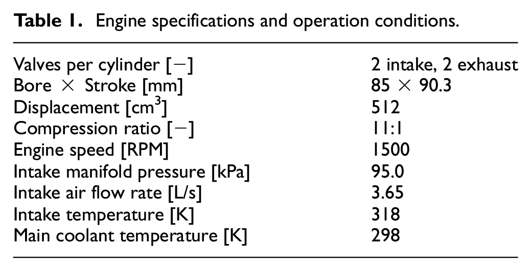
Engine specifications and operation conditions.
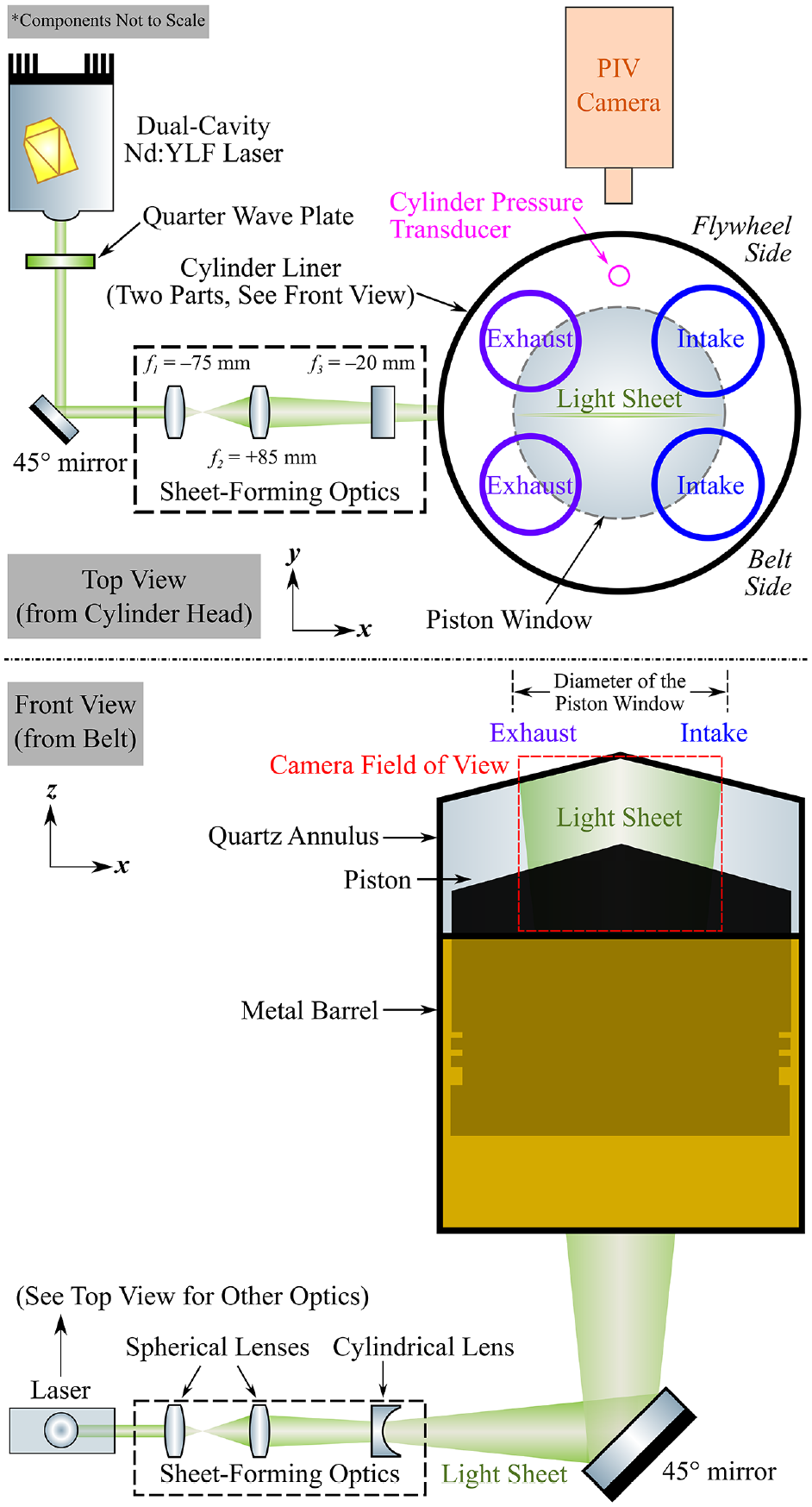
PIV setup for tumble plane flow measurement. The light sheet has a 1 mm offset towards the belt side.
The time separation between the images was controlled by a LaVision Programmable Timing Unit (Version 10) and was varied with crank angle (between 4 and 20 µs) to maintain a fixed droplet displacement between frames under different flow speeds. PIV images were processed using LaVision DaVis 8.4.0 software to generate vector fields. The camera was calibrated by imaging a reference grid placed at the location of the light sheet, and the distortion caused by the curved surface of the cylinder liner were corrected by the built-in image registration algorithm. Light reflections from the metal surfaces in the cylinder were removed via a background subtraction algorithm based on a Gaussian sliding average over multiple cycles. The intensities of the particles were normalised to compensate for their variations between individual droplet images across the field of view. The PIV vectors were evaluated by a multi-pass algorithm, of which the interrogation window reduces from 128 × 128-pixels to 32 × 32-pixels with 50% overlap in different passes.35,36 The resulting vector spacing was 0.956 mm. Local vectors with peak ratios smaller than two were removed from the final vector fields. 37 For the data set presented within this paper, the total number of removed vectors was less than 0.05%. More detailed PIV setup and data processing information have been reported elsewhere.14,34,38,39
Computational setup
The in-cylinder flow field simulation is performed using a commercially available finite-volume code package, STAR-CD, under a Reynolds-averaged Navier-Stokes framework. The turbulence is modelled using the standard RNG k-∈ approach with modified constants. A second-order spatial differencing scheme is used for the convective terms in the momentum equation; where the PISO algorithm is used for pressure-velocity coupling. A modified Angelberger model was used to incorporate heat transfer. A base grid of 0.7 mm is applied to the flow field with a refinement of 0.3 mm upstream and downstream of the intake valves. Each simulation has been performed using a grid that has a maximum of approximately 3.25 million cells at BDC. A sample port-and-cylinder mesh topology can be found in Figure 2. A variable timestep is applied during the simulation, and more details about the numerical setup and models used in the study can be found in a previous work. 38
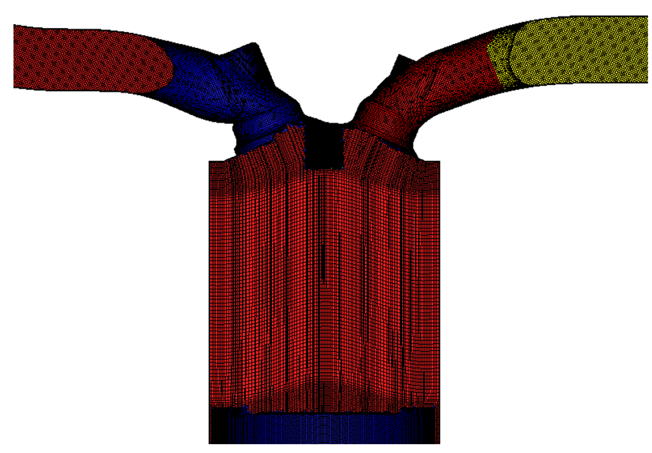
Sample CFD mesh on the tumble plane.
The working fluid in the simulation is chosen as air, which is treated as an ideal gas. Several initial and boundary conditions are adopted directly from the experimental measurements, namely:
intake and exhaust valve lifts
pressures within the inlet and exhaust runners
time-averaged intake, exhaust and main engine coolant temperatures
time-averaged intake air volume flow rate
Vector field comparison techniques
Various methods have been developed to compare CFD simulated flow vector fields to experimental data in order to assess the effectiveness of the models in capturing the physical processes. A common metric for quantifying the similarity between two in-cylinder flow fields is the Relevance Index (RI), which was introduced by Liu et al.: 40
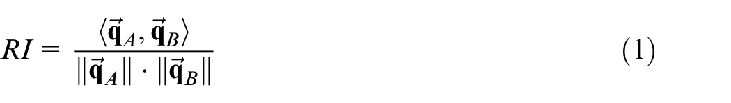
where 〈·,·〉 denotes the inner product, and ‖·‖ is the
The use of the RI provides opportunities to use a single number to quantify the differences between flow fields, both simulated and experimental. It would be useful, on the other hand, to have spatial information about how well the two flow fields are aligned and where the major differences occur. To achieve this, Chen et al. 41 and Zhao et al. 42 extended the idea of RI to point-to-point comparisons, and Zhao et al. termed it as the Local Structure Index (LSI):
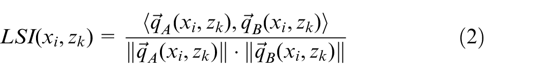
where
In-cylinder flow in a modern GDI engine is often characterised by strong tumble and/or swirl motions to enhance fuel-air mixing, and thus the in-cylinder flow fields usually contain vortixes and the flow speeds vary significantly at different locations. As the LSI has no dependence on the magnitudes of the vectors inside each field being compared, the alignment of low velocity vectors carries the same weight as that of high velocity vectors. The reversal of the flow direction and rapid flow speed change across a vortex centre cause even very small differences in the vortex centre location to result in very misaligned vectors (high local LSI values). This undesired sensitivity in the low speed regions may lead to misleading conclusions for the validity of simulation results when compared with the experimental data. Therefore, in this study new metrics developed by the authors in previous work 34 : the Weighted Relevance Index (WRI) and Weighted Magnitude Index (WMI), are used to quantify the differences between velocity fields in terms of direction and magnitude, respectively.
Weighted relevance index
The Weighted Relevance Index (WRI) quantifies vector alignments by weighting the contribution of each vector pair to an ‘alignment penalty’ by the ratio of the local velocities to the medians of the velocity magnitudes within each field:
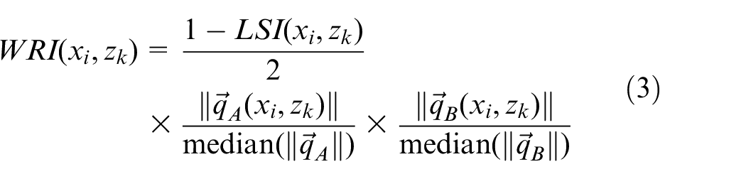
The WRI produces a field, whose values at each location are all non-negative. A lower WRI value means the two fields are aligned better at a certain grid point (Note that this is different from the standard RI, in which a lower value means the two fields have a poor overall alignment for the entire field). The spatially-averaged WRI can also be computed to produce a single value that quantifies the directional similarity between two vector fields.
Weighted magnitude index
Similar to LSI, the WRI excludes the differences in flow speed for the two flow fields. In order to quantify the magnitude alignments at each spatial location, the Weighted Magnitude Index (WMI) is introduced:
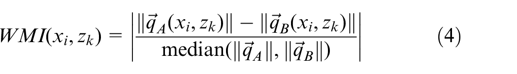
where |·| denotes the absolute value. In a similar approach to the WRI, a weighting factor is included in the definition of the WMI (equation (4)) to scale the contributions of the differences in local velocity magnitudes by the average speed of the flow field. Flow fields with similar local speeds generate low WMI values at the evaluated grid points.
PIV experiments can produce vast quantities of data, especially when they are carried through multiple engine cycles. However, most quantitative methods focus on developing metrics that can be applied to ensemble-averaged PIV data and then compare the post-processed data to the simulation. Limited approaches are available to make an objective quantitative comparison between PIV and simulations that go beyond ensemble averaging.
Post-processing manifold reduction techniques
In this section, two post-processing manifold reduction techniques, namely: linear PCA (POD) and KPCA are introduced for flow characteristics feature extraction. The mathematical relationship between linear PCA (POD) and KPCA is given. The algorithm structure and assumptions of both approaches are included in order to highlight the differences. In addition, a short summary of the strengths and weaknesses of each method is detailed.
Proper orthogonal decomposition (POD)
Proper orthogonal decomposition (POD), also known as principal component analysis in the modelling community, is used to impose orthogonal projection of data onto lower dimensional spaces (known as the principal subspace), where the variance of the projected data is maximized.
30
The projected data, also known as the reconstructed data, can, therefore, have a smaller data structure and possibly be free of noise/error. Various numerical methods can be used to perform POD and obtain the reconstructed data, including eigenvector decomposition and the singular value decomposition. In this study, the reconstructed solution is obtained from the SVD approach. For a dataset of in-cylinder PIV flow field data
where
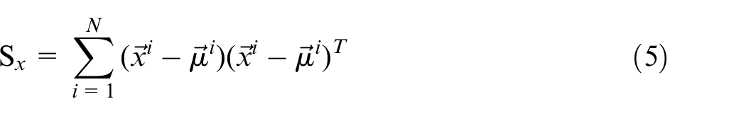
The purpose of subtracting the mean is to centre the data, therefore, converting observations into fluctuations over the mean. In order to reconstruct the data, we find the eigenvectors (
The dominant eigenvectors describe the main directions of variation of the data, which was found to contain the most significant in-cylinder flow characteristics. For example, if a dataset has d large eigenvalues, the coherent flow structure can then be described largely by linear combinations of the d corresponding eigenvectors. Define

The projection of vector

The corresponding scatter matrix

From the SVD approach, one will get the matrix
Before introducing KPCA into the picture, it is worth highlighting the assumptions made behind PCA, as well as the incentive and need for using an alternative manifold reduction to reconstruct the data:
• Linear change of basis
POD/PCA is based on a linearity assumption, meaning that linearity frames the problem as a change of basis.
• Large variances dominate structure
This assumption requires the experimental data to have a high signal-to-noise ratio (SNR). Hence, principal components with larger associated variances represent the interesting structure, while those with lower variances represent noise.
• Principal components are orthogonal
This is to allow the decomposition to be solved using linear algebra techniques
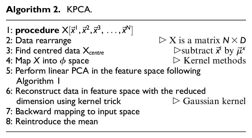
Kernel principal component analysis
Kernel principal component analysis is an alternative to the POD/PCA. The basic idea of KPCA is to non-linearly map the original data,
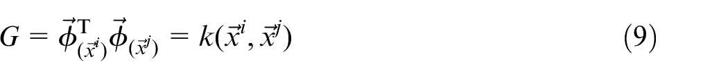
where

From equations (9) and (10) we can see that selecting some

Various choices of kernels also exist in the literature.44,45 Once the original data has been transformed to the feature space, a linear PCA can be performed to reconstruct the original data in the feature space. The detailed derivation in terms of KPCA can be found in the literature. 31
Reconstruction and pre-image
One of the major differences between PCA and KPCA is that the data used in KPCA is transformed through different kernels. When it comes to reconstruction, the same approach from PCA (equation (7)) is not feasible for KPCA anymore, as the decomposition is performed in the feature space rather than the sample space. Therefore, an additional step is required to map back the denoised low dimensional data into the original dimension. In this study, the reconstruction of Gaussian kernels is given by Wang’s method. 46 Figure 3 shows the relationship between PCA and KPCA. The full KPCA reconstruction procedure can be seen in Algorithm 2.
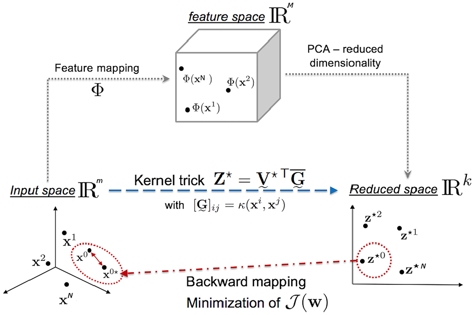
Schematics of kernel PCA. 47
Results and discussions
Before a detailed flow field characteristics study, simulated in-cylinder global characteristics are compared with the experiment. For this study, the crevice length (defined as the distance between the piston top edge and the upper piston ring) was varied for each condition to match the in-cylinder pressure trace. There was no further tuning of the physical models. The phase-averaged measured pressure trace (blue line) and simulated pressure traces (magenta line) are shown in Figure 4. A good overall match between the simulation and the experiment is observed; the CFD predicts a lower (by 3.2%) peak pressure than the PIV 300-cycle average.
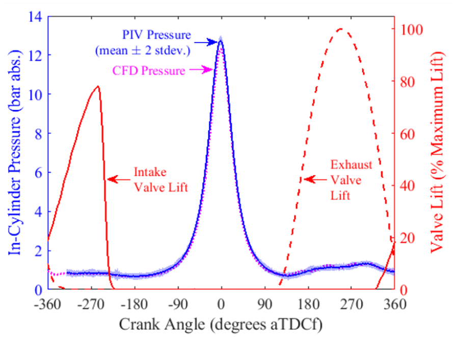
In-cylinder pressure trace comparison between the ensemble averaged PIV experiment and the RANS simulation.
RANS versus ensemble-averaged and single cycle experimental study
In this section, we first applied the widely used method of validating the RANS simulation via direct comparison with the ensemble-averaged experimental flow field. Both qualitative and quantitative results are highlighted. The ensemble mean normalized flow field at 280 CAD bTDCf with a zoomed-in plot near the jet region is compared with the RANS simulation at the same crank angle. Figure 5 shows the RANS flow field; the area marked by the red dashed line is the field of view of the experimental data.
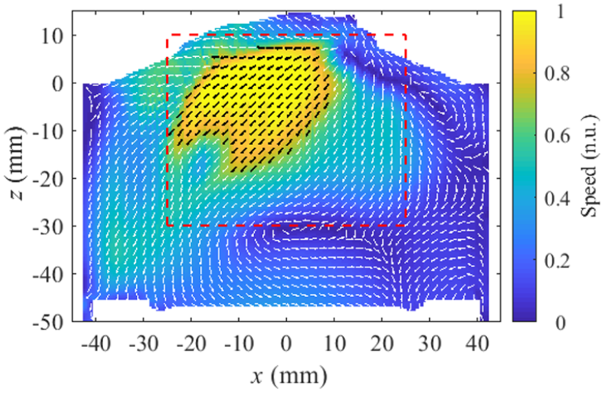
RANS CFD simulation full flow field view at 280 CAD bTDCf. The red dashed box shows the PIV field of view.
Figure 6 compares the RANS flow field (top) to both the ensemble-averaged PIV flow field (middle) and a single cycle PIV flow field (bottom) at 280 CAD bTDCf. It is worth noting that the extent of flow field is slightly different between experiments and simulation (top right corner of the experimental data is empty). This is due to the camera line of sight being blocked by the valve. Qualitatively a good match of flow field structure is seen between the simulation and the ensemble-averaged PIV experimental data, whereas the single cycle flow field shows a greater degree of small scale fluctuations as expected. However, for velocity magnitude, the ensemble-averaged PIV velocity magnitude is seen to be noticeably smaller compared to the RANS simulation and the presented single cycle PIV experimental flow field. In order to quantitatively compare the flow fields with CFD, we first calculated the widely used relevance index given by equation (1). Figure 7 shows the relevance index of the ensemble-averaged PIV and all single cycle PIV results over the RANS CFD simulation. The figure shows that when comparing with the CFD the ensemble-averaged flow gives better matched results compared to all single cycle data sets. However, as mentioned before, the standard relevance index does not retain spatial information which can inform where the flow fields match well or poorly and differences in both direction and magnitude contribute to the RI values.
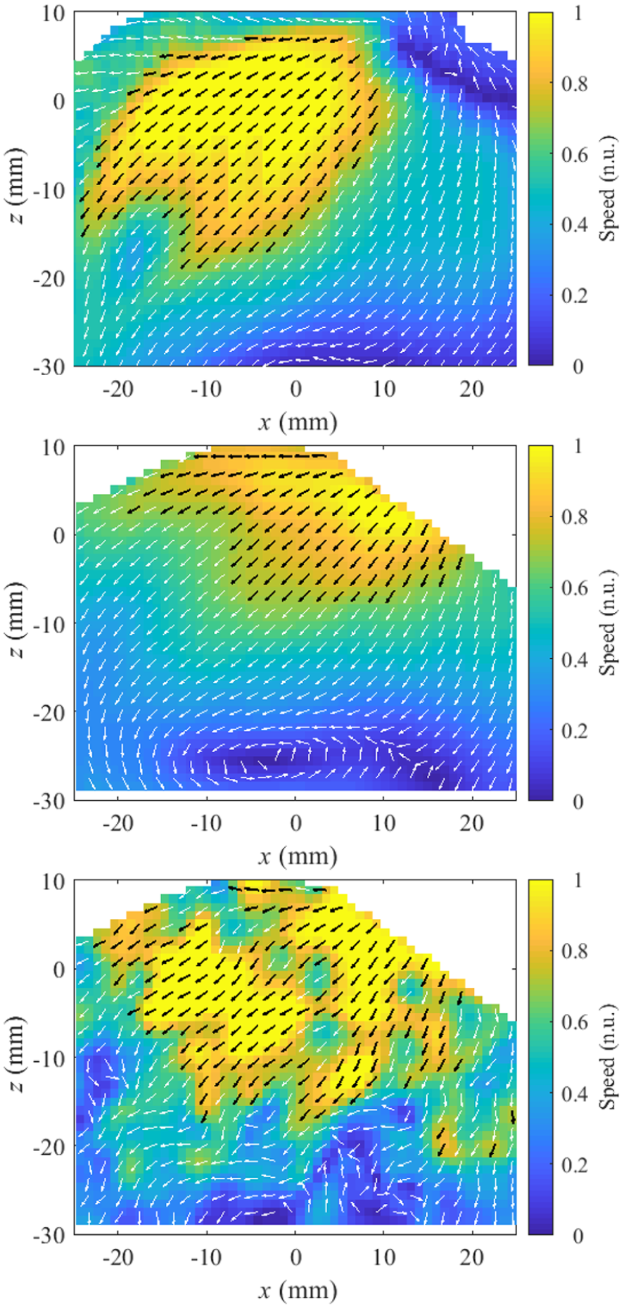
Zoom in CFD simulation normalized flow view (top) compared with 300 cycles ensemble-averaged PIV normalized flow field (middle) and a single cycle PIV flow field (bottom) at 280 CAD bTDCf.
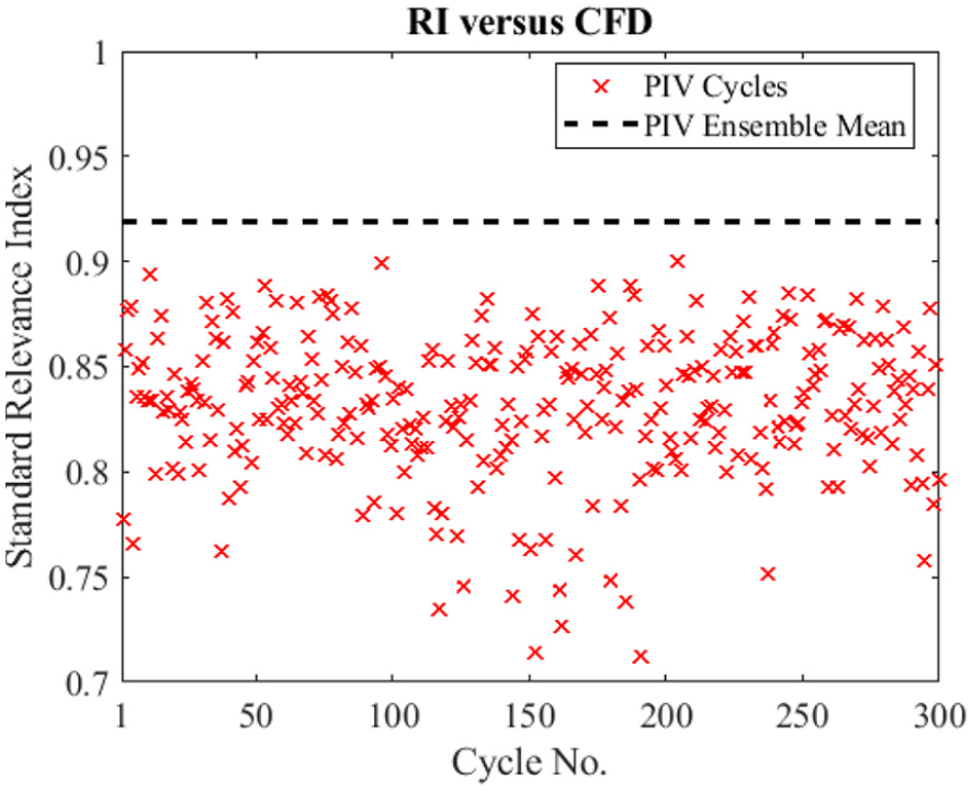
Standard relevance index for all 300 individual experimental PIV cycles and PIV ensemble mean comparing to the CFD data at 280 CAD bTDCf.
In order to investigate differences in direction and scalar magnitude independently in the study, the above-mentioned weighted magnitude index and weighted relevance index are used to quantify the differences between the simulation and the experiments. For qualitative comparison, Figure 8 shows the WRI and WMI fields for comparison of the ensemble-averaged and the selected individual cycle experimental flow fields over the RANS simulation (note: for each index a lower value indicates a better match with the CFD simulation). From WRI, the simulated flow field has a better directional match with the ensemble-averaged results. The chosen cycle is seen to have a relatively close WRI with the ensemble-averaged experimental data. Differences are found in the intake jet region where small regions within the single cycle flow field show varying direction to the ensemble mean. This is expected that neither the ensemble-averaged experimental data nor the RANS simulation is not able to capture small eddies. However, when comparing WMI, the ensemble-averaged flow field is seen to have a higher degree of difference in magnitude of the core flow. Qualitatively, the individual cycle is seen to have a better match with the RANS simulation.
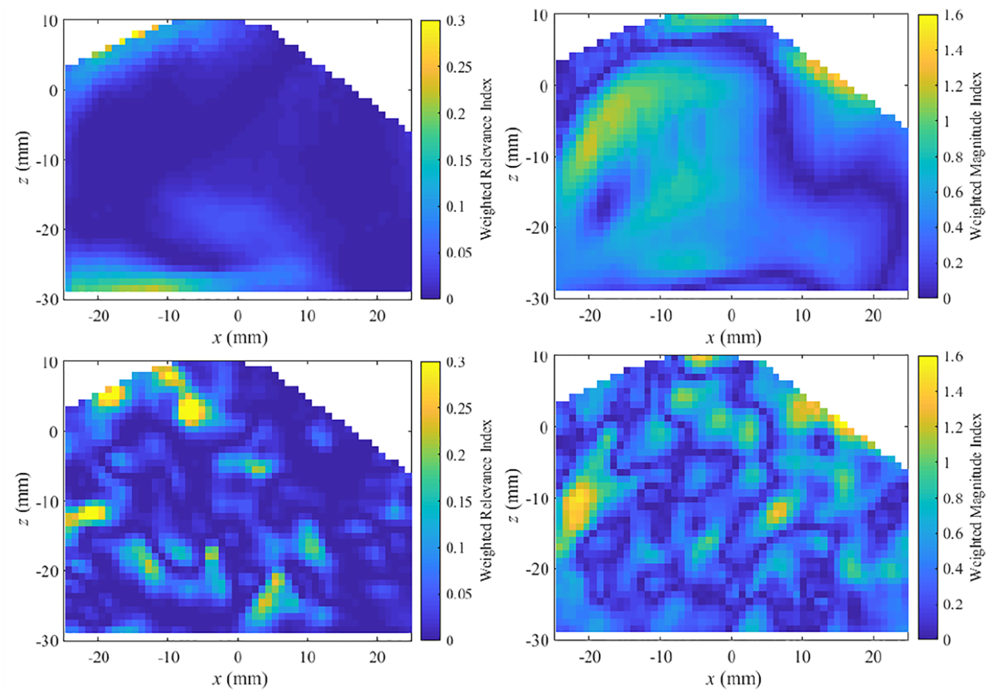
Weighted relevance index (left column) and weighted magnitude index (right column) for ensemble-averaged PIV (top row) and individual experimental PIV flow field (bottom row) compared with the CFD data at 280 CAD bTDCf.
Figure 9 shows the spatially-averaged WMI and WRI for each individual PIV cycle and ensemble-averaged PIV results compared with the RANS simulation. When calculating WMI for all 300 cycles of experimental data with the RANS simulation, a better agreement is found for a number of individual cycles compared to the ensemble-averaged experimental data. Previous studies with similar results suggested that the mean convective term in RANS formulation contributes to a rapid rise in scalar terms, whereas an ensemble-averaged field from the experiment is smoothed both in time and space, therefore giving lower magnitude. One might assume that RANS will have better a similarity with the ensemble-averaged quantities; however, from this study, an individual cycle is found both qualitatively and quantitatively to match better with an experiment in terms of scalar magnitude. This would suggest a further adjustment in RANS simulation is needed if the aim is to match the part of the flow that has been reduced from the turbulent fluctuations. Although a good WMI is observed from various single cycle experiments in the intake jet region, one would argue the differences in direction between the individual cycle experiment and the RANS simulation is significant which makes it essential to also calculate the averaged WRI for all 300 cycles. When comparing the WRI for all cycles, however, a poor agreement is observed via a single cycle flow field compared to ensemble-averaged flow fields. The more fluctuating nature of the flow field in a single cycle experiment makes it virtually impossible to have a good match with the RANS simulation in terms of vector field directions. From the WMI and the WRI study, we can conclude both qualitatively and quantitatively that a comparison using either single-cycle experimental data or ensemble-averaged experimental data might not be appropriate for RANS simulation validation especially when cycle-to-cycle variations are present. Therefore, alternative tools might be needed to determine whether the structure or the magnitude are reliably captured by RANS simulations.

Weighted relevance index and weighted magnitude index for all 300 individual experimental PIV cycles and ensemble-averaged PIV experiment compared to the RANS CFD simulation at 280 CAD bTDCf.
POD (linear PCA) analysis
Proper orthogonal decomposition (POD) has been proposed as an approach to make objective quantitative comparisons between PIV and LES that goes beyond ensemble averaging. POD can provide insights into in-cylinder flow dynamics and can be used to quantify CCV of in-cylinder flows. A previous study has also suggested possible usage of POD combined with other quantitative criteria on experimental data for the validation of a RANS simulation. 14 In this section, we applied the commonly used POD analysis procedure to compare the experimental data with the RANS simulation. Given the mathematical process of SVD after centering the data, the 300 cycles data set would have 299 POD modes with a decreasing amount of kinetic energy captured by each successive mode.
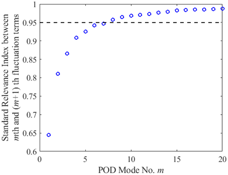
In order to choose the number of modes needed to reconstruct the flow fields, the previously mentioned quadruple POD method is applied here where the turbulent flow field is decomposed into four separate classes: mean, coherent, transition and turbulent flow motion. The coherent flow motion contains large-scale vortices and plays a critical role in the CCV. The transition part is identified as a passage in the energy cascade between the large-scale vortices in the coherent turbulence and the smallest ones in the incoherent background turbulence. The turbulent part here represents the small-scale structures in the flow field, which are homogeneous and isotropic. There are different criteria that can be used as the cut-off for different flow motions. Qin et al. 48 proposed using the correlation coefficients among the reconstructed flow fields where a RI = 0.95 threshold corresponds to the cut-off number between coherent flow motion and transition flow motion. For this study, the number of POD modes required is determined by the RI between the fluctuation flow structure reconstructed by the first m modes and the flow structure using one additional mode (i.e. using the first (m + 1) modes). 24 If the addition of a POD mode to the flow reconstruction does not modify the resulting field significantly, that is, if the RI is close to 1, the contribution of that POD mode is negligible. Therefore, the cut-off number can be identified for the coherent part of the turbulence. Figure 10 shows the averaged RI over 300 cycles with an increasing number of modes at 280 CAD bTDCf. A RI over 0.95 is achieved when 8 POD modes are included in the calculation. Figure 11 shows reconstructed POD flow fields (ensemble mean plus the fluctuation flow structure) for two different cycles (left: cycle A and right: cycle B) where the flow fields are presented side by side using the same number of modes. Although no direct physical correlation is to be drawn from the first mode, the reconstructed flow field for the first mode qualitatively shows a high degree of similarity with the ensemble-averaged experimental flow field. The CCV of the flow field can be seen with the addition of increasing number of POD modes until with 299 modes the reconstructed flow field is identical to that the original single cycle flow field. It is worth noting, for the POD method, every mode included in the reconstruction process will contribute to a change in the flow field behaviour. For instance, differences in flow structures can be observed between 5 and 8 modes (the third versus the fourth row in Figure 11), as well as between 8 and 20 modes (the fourth versus the fifth row). Therefore, choosing the correct number of modes for the reconstruction is critical.
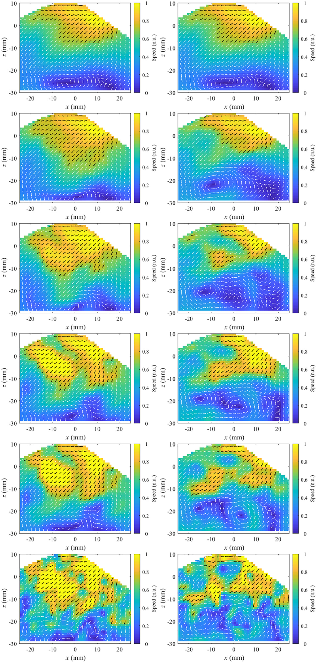
POD-based reconstruction for two individual cycles (left: cycle A and right: cycle B) at 280 CAD bTDCf. Different numbers of modes are included in the reconstruction for each row. First row: ensemble mean, second row: 1 mode, thirdrow: 5 modes, fourth row: 8 modes, fifth row: 20 modes and last row: 299 modes (original cycles).
A quantitative comparison of the POD reconstructed flow field using 8 modes with the simulation is performed where the WRI and WMI of cycle A over the RANS simulation are given in Figure 12. For cycle A (also shown in Figure 6), an improvement in WMI is given by the POD reconstructed flow field compared to the ensemble-averaged PIV results. There are two regions in the flow field where WMI is seen to be higher, which is related back to the CCV of the flow field where in those regions pockets of low velocity region exists. For the reconstructed flow field WRI, a great improvement is achieved compared to the individual experimental cycle over the simulation. The quantitative analysis shows the capability of the POD reconstructed flow field not only in capturing the main flow field information (ensemble average information) but also in including the coherent flow field structure where CCV is found to be most relevant.
WRI (left) and WMI (right) for POD reconstructed cycle A flow field compared to the RANS simulation.
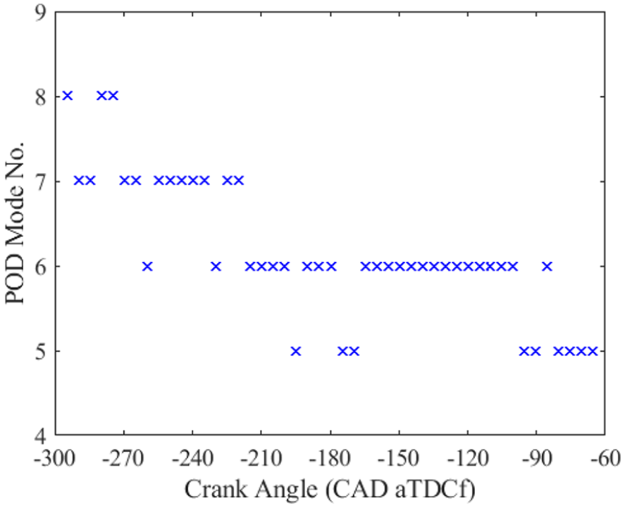
Although the reconstructed flow field using the chosen eight modes has shown both quantitatively and qualitatively better validation for the RANS flow field, one key question remaining to be answered would be, how are these results related to the number of modes chosen for the reconstruction? In order to study this, we have included all other crank angles for the analysis where similar RI criteria are used to choose the number of modes needed for the POD analysis. Figure 13 shows the number of modes needed for various crank angles of reconstructed flow fields to reach a RI over 0.95. The results indicate a difference in the number of POD modes needed to reach the same criteria, which varies from 5 to 8 modes. Although the difference in the number of modes is only 1% of the available 299 modes, the POD reconstructed flow field in Figure 11 shows that the inclusion of even one additional mode in the POD analysis can produce a distinct change in the reconstructed flow field. Similar results in the literature also indicate the same challenges faced with the POD method,26,49 especially when there exists more than one criteria to determine the number of modes. Therefore, how many POD modes should be included in the reconstructed data to represent the coherent flow structure, without introducing small-scale turbulence that may bias its comparison with the RANS modelled data still remains a challenge. Additionally, as mentioned before, Figure 10 gives only the averaged RI for all cycles at a fixed crank angle. Figure 14 shows the RI error band for all individual cycles, where a wide range of RI is observed for each chosen mode over 300 cycles. For certain cycles, the RI might not reach 0.95 using the chosen mode, which creates another layer of uncertainty in using such a selection criterion. With this in mind, we proceed the study by focusing more in terms of what is the inherent structure hidden in the data that can be used as a tool to create an objective selection criterion.
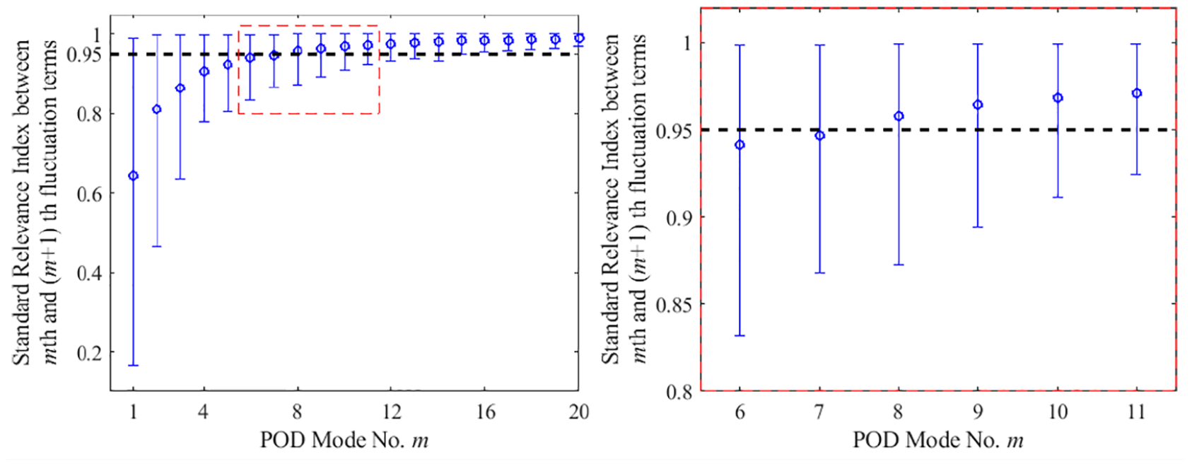
RI error band for varying number of modes with 300 individual PIV cycles at 280 CAD bTDCf. Blue circles: mean; error bar bounds: 10% and 90% quantiles.
Statistical analysis on a single crank angle
Previous studies have found that it is difficult to define an objective criterion to identify the cut-off number of modes between coherent and incoherent turbulence in the POD method. Studies have suggested that homogeneous isotropic turbulent flows follow Gaussian properties where converged skewness and flatness coefficients on the velocity fluctuation can help to identify an objective cut-off number. 17 With this in mind, in this study, the 300 cycles velocity distribution of the entire flow field from the experimental measurements is first examined.
In order to examine the flow field vector distribution over the 300 cycles, a statistical test is needed: the chi-squared (
where
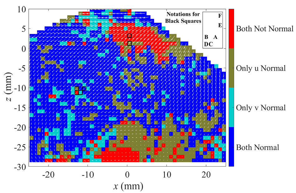
Chi-squared test for normality at 280 CAD bTDCf with a significance level (p value) chosen as 0.05. Red indicates both u and v velocity components rejected the null hypothesis of having a normal distribution at the chosen significance level. Green shows only u component accepted the null hypothesis. Grey shows v component accepted the null hypothesis and blue indicated both components are showing normal distribution.
To further examine the Gaussian properties of the flow field the distributions of velocity components at different locations marked in Figure 15 are analysed. Example locations where the velocity components passed both, one or no chi squared tests are highlighted in two regions: the bulk flow region (Figure 16) and the intake jet region (Figure 17). Figure 16 shows the distribution of both horizontal and vertical velocity components of 4 locations in the bulk flow. The normal distribution is fitted to the data in red line where the null hypothesis for a chi-squared test is that the hypothesized distribution of a scalar is a normal distribution. Therefore, for any p value greater than 0.05 will indicate that the scalar distribution is close to a normal distribution. The CCV of the flow field can be observed from all locations in the flow field. For all locations plotted here, even though some of the locations have failed the hypothesis criteria (p < 0.05), it can be seen that qualitatively the deviations from a normal distribution are not severe. These findings echo with the previously mentioned study where homogeneous isotropic turbulent flows were found to follow Gaussian properties. 15 As seen from the statistical study, for this flow condition, a non-linear correlation exists in the flow field. Therefore, mapping the data using a Gaussian distribution onto a higher dimensional space could help to flatten the non-linearity that has been exhibited.
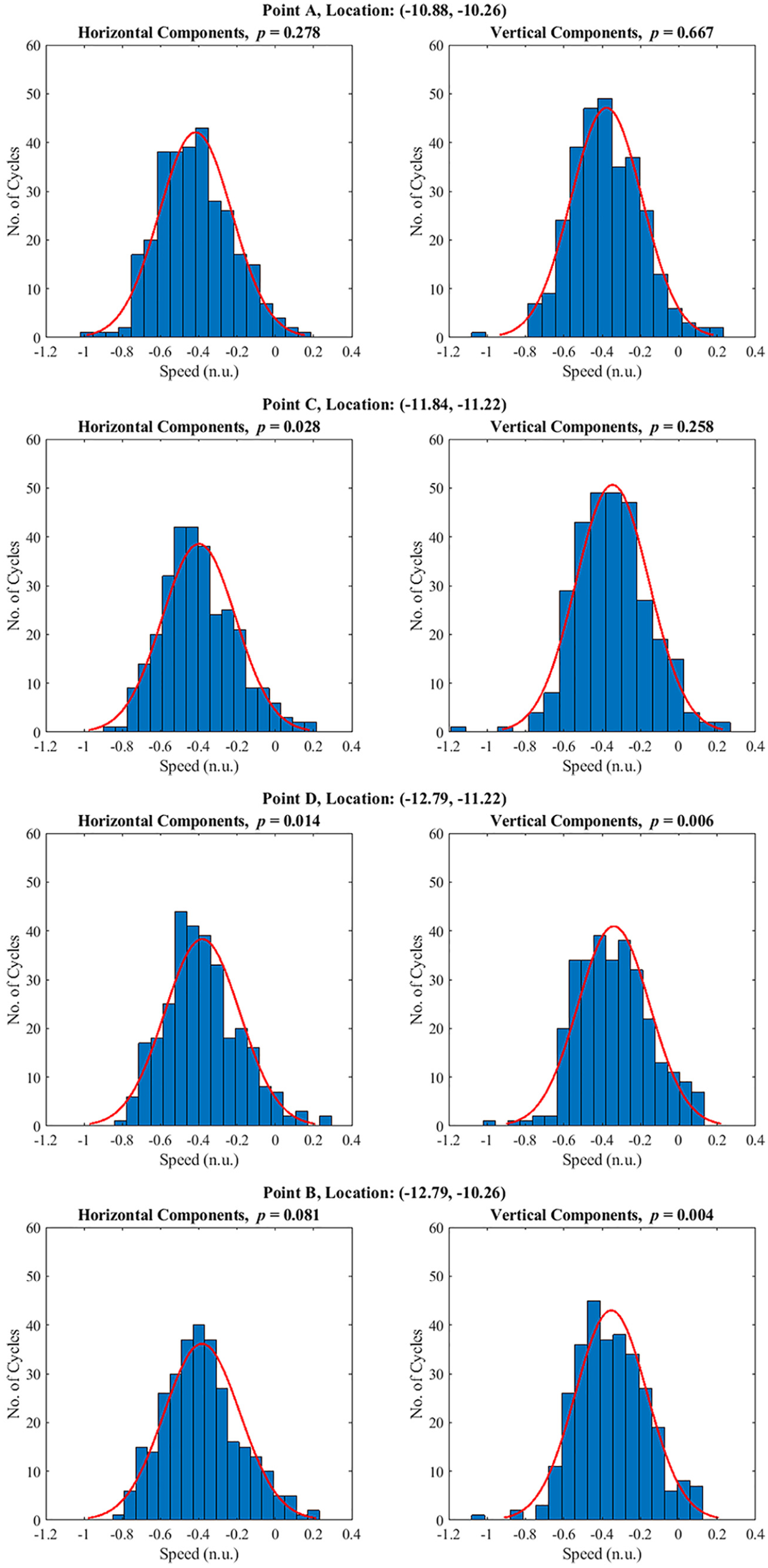
Single point bulk flow velocity components distributions at 280 CAD bTDCf, left:horizontal velocity component, right: vertical velocity component. The red line shows a normal distribution fit of each histogram. The location of the each analyzed point is marked in Figure 15.
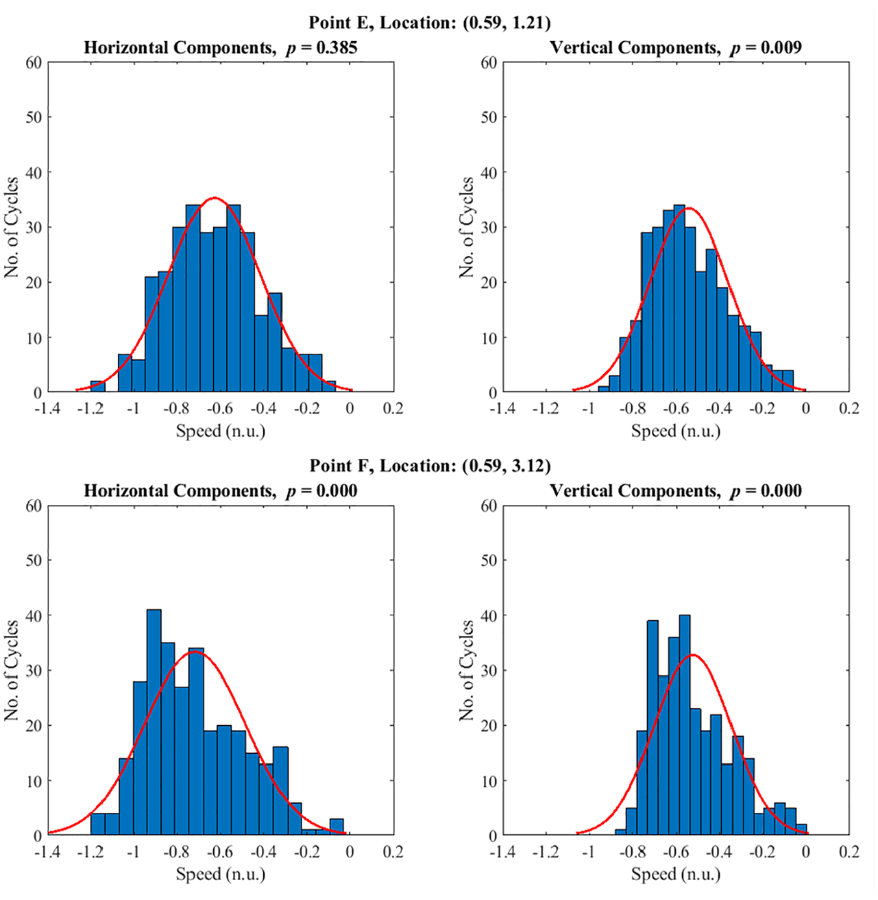
Single point intake jet velocity components distributions at 280 CAD bTDCf, left:horizontal velocity component, right: vertical velocity component. The red line shows a normal distribution fit of each histogram. The location of the each analyzed point is marked in Figure 15.
Application of KPCA
From a statistical analysis of the flow field, we observed that there exist strong Gaussian properties in the velocity components. Therefore, when considering manifold reduction techniques, a non-linear option might be more attractive. Kernel PCA offers an opportunity to map the data into a chosen non-linear space. A Gaussian kernel is chosen for this study, and is given by:
Following the procedure given by Figure 3, the full dataset is first mapped into a high-dimensional non-linear space where the Gaussian distribution is flattened. In that space, we performed a linear dimensional reduction technique (PCA) which is identical to the POD analysis. The flow field is reconstructed first with various number of modes in the non-linear manifold space and then projected back to the original physical space. The resulting flow field is given in Figure 18 for two different cycles (left: cycle A and right: cycle B) with the same number of modes used in each row. Similar to the POD reconstructed flow field, the first mode given by the KPCA method resembles closely the ensemble-averaged PIV data, and the flow fields start to deviate from the ensemble mean as more modes are included in the reconstruction. Differences are seen compared to the POD reconstructed flow field when a higher number of modes are used. For POD reconstruction (Figure 11), the flow field will continue to gain features when the number of modes is increased until the flow field is completely reverted to the original flow field. However, for the case of KPCA, a clear convergence of the final reconstructed image is given. As seen in the last three rows of Figure 18, where reconstructed figures are given by 8, 20 and 100 modes respectively, limited changes in the main flow field can be seen in these figures. Some changes on the flow field periphery are observed, which are likely caused by the numerical rounding in the reconstruction process.
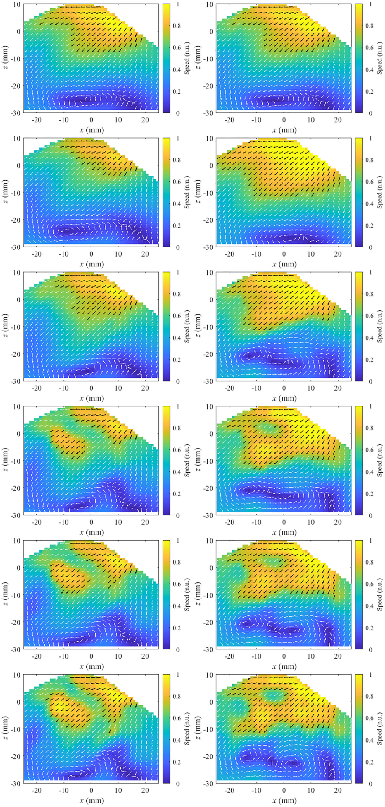
KPCA reconstructed flow field for two individual cycles (left: cycle A and right: cycle B) at 280 CAD bTDCf. Different numbers of modes are included in the reconstruction for each row. First row: ensemble mean, second row: 1 mode, third row: 5 modes, fourth row: 8 modes, fifth row: 20 modes and last row: 100 modes.
Figure 19 further shows that when increasing the number of modes to reconstruct the flow field via the POD method, typically a continuously decreasing trend occurs in the RI compared to CFD data for each additional mode. This is consistent with previous POD reconstruction PIV studies 26 as well as theoretical studies where eigenvalues of the covariance matrix were found to form a more continuous spectrum, so that any sharp division between important and unimportant dimensions would be arbitrary when using POD or linear PCA-based models to perform the dimensional reduction in original data. 22 For the KPCA reconstructed flow field, the RI (versus CFD data) will eventually reach or approach a constant (respectively for different cycles, see Figure 19) with a large number of modes. This is likely to be owing to the flattening of the non-linear data in a Gaussian space, where data with a high variance away from the Gaussian behaviour is directly filtered. This also explains why the last two rows of Figure 18 show minimal differences despite increasing the number of modes by a factor of 5.
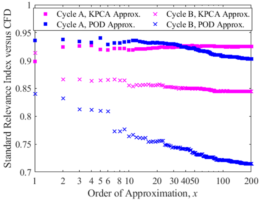
RI versus CFD data for POD (blue) and KPCA (magenta) reconstructed flow fields with varying orders of approximations at 280 CAD bTDCf.
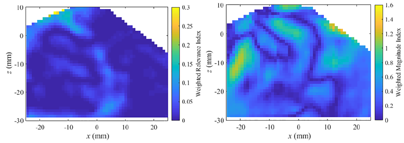
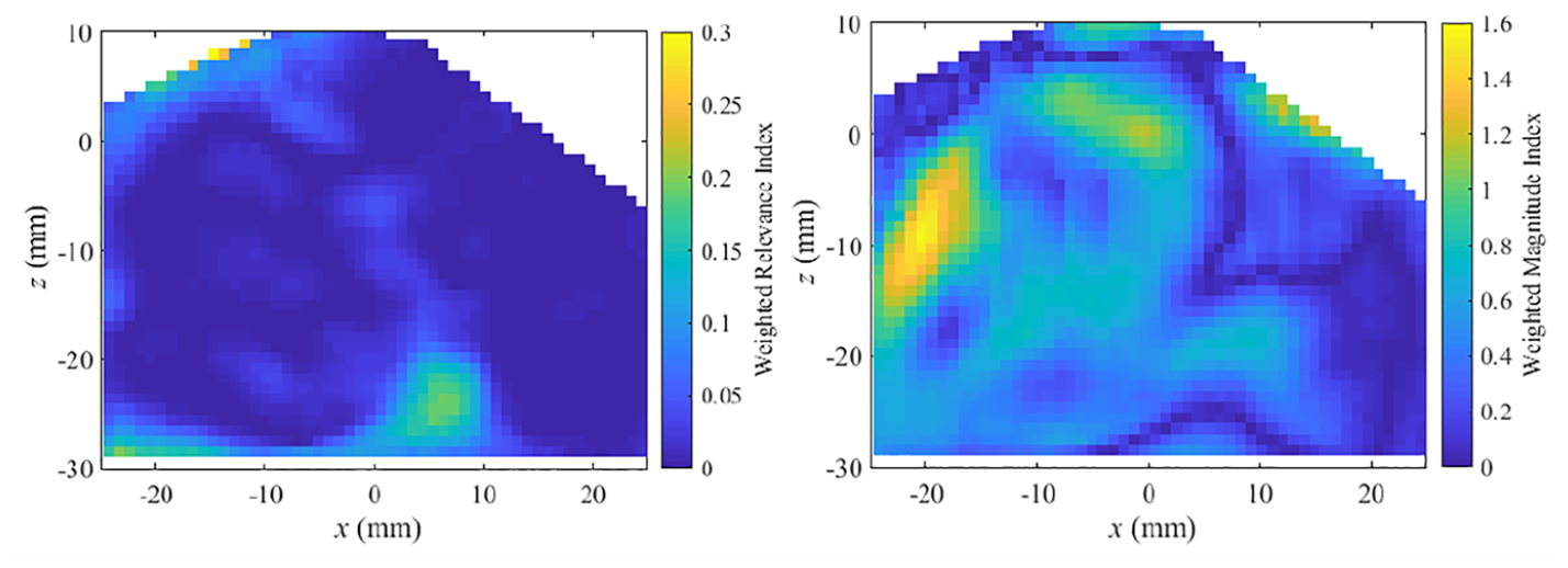
The reconstruction of the flow field using the KPCA method has shown an advantage in terms of converging results. Therefore, it is essential to check whether using such a method would decrease or increase the level of agreement with the RANS CFD data compared to ensemble averaged flow field or POD reconstructed flow field. Figure 20 shows the WRI and WMI for the KPCA reconstructed cycle A flow field. For the WRI, a slight higher region is spotted at the bottom of the flow field, which is due to the vortex induced by the flow. This was also highlighted in the statistical study where in this region, a weaker Gaussian distribution of the flow field is present. The WRI shows a significant improvement compared to the individual cycle comparison shown in Figure 8. For the WMI, a slight improvement is given by the KPCA reconstructed flow field where the characteristics of the single cycle flow field were accurately incorporated leading to a region with improved WMI. When compared to the results from POD reconstructed flow field shown in Figure 13, qualitatively no significant differences are given which corresponds well with the quadruple POD analysis. As for this particular cycle, the flow field has a relatively high similarity to the RANS flow field.
WRI (left) and WMI (right) for cycle A KPCA reconstructed flow field compared to RANS simulation at 280 CAD bTDCf.
Finally, the quantitative comparison between different methods for validating the RANS simulation is made. Here the POD reconstructed flow field is given by the modes determined by the quadruple POD analysis whereas the number of modes used in the KPCA method is chosen as 20 (minimal differences exists varying from 20 to 100 modes as seen in Figure 19, however, for computational efficiency, a smaller value is chosen). Figure 21 shows the WRI and WMI for all four different ways of validating the RANS simulation. Both KPCA and POD reconstructed flow fields can incorporate CCV in individual experimental PIV flow fields. A significant improvement was seen in terms of the WRI and WMI. When comparing these two methods, limited differences are found in WRI and WMI over all cycles, which shows that both methods can be used to incorporate CCV while validating the RANS simulation. However, the KPCA has a significant strength due to its rather more clear-cut mode selection process when the experimental scalar shows Gaussian properties.
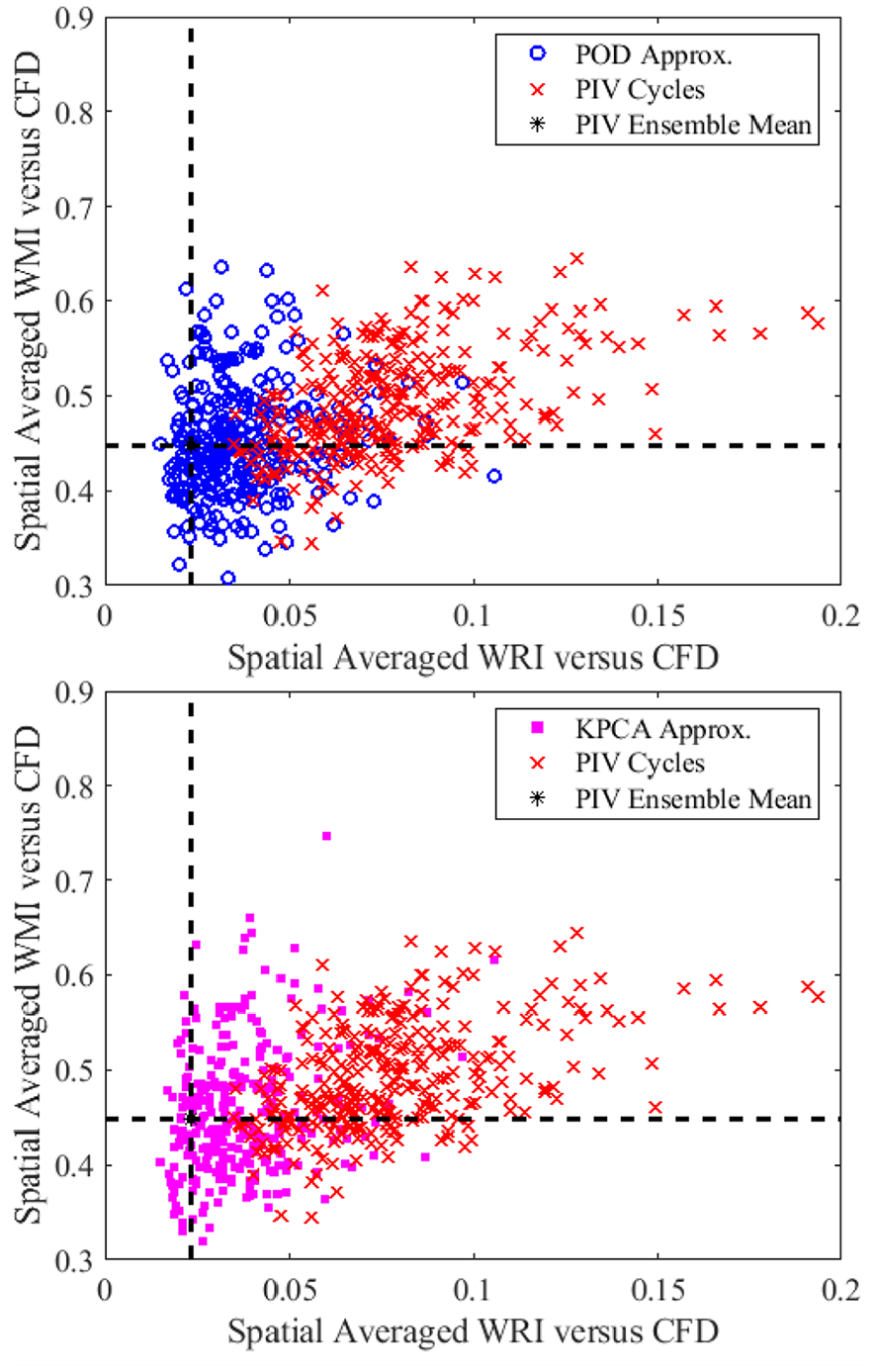
Spatially-averaged weighted relevance index and weighted magnitude index for all 300 individual experimental PIV cycles (red crosses), the ensemble-averaged PIV experiment (intersection of the two dashed lines, also shown as a black star symbol), the POD reconstructed flow field (blue circles, top figure) and the KPCA reconstructed flow field (magenta squares, bottom figure) comparing to the RANS simulation at 280 CAD bTDCf.
Conclusions
With the development of high-speed particle image velocimetry experimental techniques and computational methods for SIDI engines, it is now possible to significantly shorten the complex engine design process. However, when the flow field exhibits a high degree of variability, challenges were found in accurately comparing the experiment and the simulation. It is, therefore, critical to find methods to accurately process the data. In this study, the authors first evaluated the accuracy of traditional methods in validating the RANS stimulated flow field via either ensemble averaged experimental data or individual experimental flow fields. The results suggested neither one of them is sufficient to validate the simulation results. While the ensemble averaged experimental flow field shows good agreement for the main flow structure, no cycle to cycle variation can be included in the ensemble averaged flow field. Additionally, using an ensemble averaged flow field to validate the RANS simulation could result in a lower overall flow field magnitude than is observed in individual PIV images.
To help to validate the RANS simulation, two different manifold reduction methods are proposed here to incorporate CCV in individual cycles while capturing the main flow structure. First, the proper orthogonal decomposition method is applied to each cycle at a fixed crank angle, therefore, helping to make an objective quantitative comparison between the PIV and the RANS simulation. Using quadruple POD analysis, the number of modes is determined based on the relevance index reaching 0.95 when adding additional modes. The POD reconstructed flow field shows a quantitative improvement in terms of the weighted relevance index and weighted magnitude index, while CCV can also be captured by the POD reconstructed flow field. Although the POD method shows improvements both qualitatively and quantitatively, a well known challenge exists when determining the number of modes needed for each crank angle and each cycle. The inherent numerical process in the POD method also makes it critical to choose appropriate criteria as the reconstructed flow field varies significantly with a different number of modes. The current study used previously developed quadruple POD analysis where the separation of the main flow field is based on the relevance index, for which a different number of modes were needed when varying the crank angle. A varying RI was also found for different cycles at a fixed crank angle which makes objectively choosing a fixed number of modes for flow field reconstruction challenging.
To investigate possible ways to objectively choose the number of modes needed for the POD reconstructed flow fields, a statistical analysis has been performed on the scalars within the experimental field of view. For the tumble plane at the investigated condition during the intake process, a Gaussian distribution over 300 cycles was found across the majority of the flow field. Therefore, a non-linear variation of principal component analysis (PCA), kernel principal component analysis (KPCA), was for the first time used as a post-processing tool to reconstruct the flow field. The use of KPCA allows flattening of the non-linear Gaussian correlation between the cycles in a higher dimensional manifold where a linear PCA can be used to reconstruct the flow field. Limited changes are observed in the KPCA reconstructed flow field when a large number of modes are chosen. A qualitative study also indicates that the KPCA is indeed capable of capturing the main flow field for each cycle while incorporating CCV. Further quantitative study also indicated that without using dedicated criteria to choose the number of modes, the KPCA reconstructed flow field could have comparable accuracy to the POD reconstructed flow field with the chosen number of modes. This indicates that KPCA can be a promising post-processing candidate for validating RANS simulations when a large number of engine cycles, crank angles and engine conditions are needed for the development of a new engine. Further studies will focus on flow fields exhibiting other statistical distributions.
Footnotes
Acknowledgements
The authors would like to thank EPSRC and Jaguar Land Rover Limited for their financial support and Dr. Blane Scott (our previous group member) for his efforts in the PIV experiments. Additionally, the authors would like to acknowledge the use of the University of Oxford Advanced Research Computing (ARC) facility in carrying out this work.
Declaration of conflicting interests
The author(s) declared no potential conflicts of interest with respect to the research, authorship, and/or publication of this article.
Funding
The author(s) received no financial support for the research, authorship, and/or publication of this article.