Evaluation of residual gas fraction estimation methods for cycle-to-cycle combustion variability analysis and modeling

Abstract

Cycle-to-cycle combustion variability in spark-ignition engines during normal operation is mainly caused by random perturbations of the in-cylinder conditions such as the flow velocity field, homogeneity of the air-fuel distribution, spark energy discharge, and turbulence intensity of the flame front. Such perturbations translate into the variability of the energy released observed at the end of the combustion process. During normal operating conditions, the cycle-to-cycle variability (CCV) of the energy release behaves as random uncorrelated noise. However, during diluted combustion, in either the form of exhaust gas recirculation (EGR) or excess air (lean operation), the CCV tends to increase as dilution increases. Moreover, when the ignition limit is reached at high dilution levels, the combustion CCV is exacerbated by sporadic occurrences of incomplete combustion events, and the uncorrelation assumption no longer holds. The low or null energy released by partial burns and misfires has an impact on the following combustion event due to the residual gas that carries burned and unburned gases, which contributes to the deterministic coupling between engine cycles. Many residual gas fraction estimation methods, however, only address the nominal case where complete combustion occurs and combustion events are uncorrelated. This study evaluates the efficacy of such methods on capturing the effects of partial burns and misfires on the residual gas estimate for high-EGR operation. The advantages and disadvantages of each method are discussed based on their ability to generate cycle-to-cycle estimates. Finally, a comparison between the different estimation techniques is presented based on their usefulness for control-oriented modeling.

Introduction

Spark-ignition (SI) internal combustion engines dominate the current light-duty vehicle market, corresponding to 94% market share. In recent years, battery electric vehicles and plug-in hybrid electric vehicles have steadily gained market penetration. However, the U.S. Energy Information Administration (EIA) forecasts that gasoline vehicles will remain the dominant vehicle type through 2050. ¹ Consequently, increasing the efficiency of SI engines can substantially improve the fuel economy of the light-duty sector in the near- to mid-term future and reduce the impact of the transportation sector on climate change.

Dilute combustion, accomplished either by excess air or with exhaust gas recirculation (EGR), is a technologically proven and cost-effective way to improve fuel economy on a broad scale. The efficiency gain comes primarily at part load via improved gas properties, decreased throttling losses, and decreased heat losses. ² Even though the knock mitigation can be substantially reduced for highly boosted conditions, significant efficiency advantages remain at less aggressive boost pressures.^3,4 In this study, cooled EGR was used to dilute the stoichiometric air-fuel charge, which allows the usage of a conventional three-way catalyst for emission control. As dilution levels increase toward the ignition limit, however, the engine efficiency is affected by sporadic partial burns and misfires.^5,6 Therefore, the ignition limit, also known as misfire limit, determines the conditions of maximum fuel efficiency under EGR dilution. Although previous research has focused on the estimation of such a limit in order to use feedback control to minimize fuel consumption, complete avoidance of misfires and partial burns remains an open problem.^7,8

The cycle-to-cycle variations that occur at the dilute limit have been shown to combine stochastic (or unobservable) variations such as turbulence and local mixture inhomogeneity at the spark plug with deterministic effects caused by the cycle-to-cycle coupling of initial composition through residual gases.^9–11 The extension of the ignition limit can thus be accomplished by predictive control strategies that anticipate such events and perform corrective control commands before partial burns and misfires occur. Existing models for the deterministic causes of these variations capture the effect of the residual gas composition, but either assume constant (or only stochastically varying) residual gas fraction ⁹ or rely on models that are too computationally expensive for real-time control applications. ¹² Modern control methodologies, however, require the development of models that correctly capture the dynamic evolution of the thermodynamic states in the combustion chamber with low computational complexity.^13,14 Accurate estimation of cycle-to-cycle changes in the residual gas fraction as well as composition is thus needed to capture the dynamics of these states.

According to the U.S. Driving Research and Innovation for Vehicle efficiency and Energy sustainability (DRIVE) partnership, a significant barrier that inhibits the widespread introduction of dilute combustion engines is the incomplete understanding of the cycle-to-cycle combustion variability dynamics that results in sporadic partial burns and misfires. ¹⁵ This study assumes that the dynamic coupling between combustion cycles is caused by the composition of the residual gas available at the beginning of every combustion cycle, as previously introduced by Daw et al. ⁹ Under such an assumption, the residual gas composition available for the next combustion cycle depends on the combustion efficiency and the residual gas fraction of the previous cycle. The combustion efficiency can be directly calculated by the energy balance during combustion. The residual fraction, however, must be estimated using different sets of assumptions. This paper presents an exploratory study regarding residual fraction estimation methods that can be used for control-oriented modeling of cycle-to-cycle combustion dynamics at the ignition limit. In order to do so, experimental engine data were collected to estimate the empirical values of the combustion efficiency and residual gas fraction. For each residual fraction estimation method, a control-oriented model was calibrated and simulated. Finally, experimental and simulated values were compared to determine which residual gas fraction estimation method yields the most accurate model for offline simulation.

The residual fraction estimation methods presented here can be classified, based on their main assumptions, into two categories: (1) methods that consider an ideal thermodynamic cycle,^6,16 and (2) methods that consider only the exhaust process.^17–19 Methods using the first set of assumptions solve the entire thermodynamic cycle under ideal conditions. Those using the second set of assumptions consider only events between exhaust valve opening (EVO) and exhaust valve closing (EVC). Other methods have been proposed in the literature that either use the intake process or the combustion process to estimate the total trapped mass and deduce the residual fraction.^20,21 During the compression stroke, there is a linear correlation between steady-state cylinder flow and in-cylinder pressure changes. However, Worm showed that this method is only valid for estimating the average trapped mass and does not generate cycle-to-cycle estimates. ²⁰ Mladek and Onder proposed a method to estimate both the total trapped and residual mass using the thermodynamic states at 50% mass fraction burned (CA50). ²¹ However, the in-cylinder temperature and gas properties for CA50 need to be known a priori and engine-specific correlations were used to calculate thermodynamic states throughout the cycle. Hence, only the methods corresponding to ideal cycle or exhaust process analysis were considered for this study.

The remaining sections are organized as follows. The experimental setup is first presented. The methodology of different residual gas fraction estimation methods is presented, emphasizing on the behavior of sequential combustion events. The control-oriented model considered for this study is next presented, which requires the identification of a parametric function for the residual gas fraction. The results for each estimation method are discussed focusing on the parameters needed to develop the control-oriented model. The resulting parametric functions for offline residual gas simulation are combined with the control-oriented model and each method is evaluated based on their accuracy to capture the observed stochastic and dynamic properties of combustion events. Finally, the paper presents conclusions and outlook.

Experimental setup

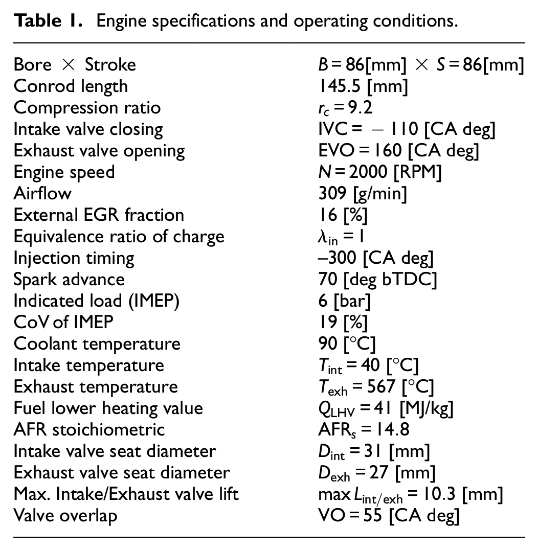
The data presented in this study were collected from a single-cylinder version of a 2.0 [L] GM Ecotec LNF engine. The experimental engine is gasoline, spark-ignited, direct injection, with four valves per cylinder (two intake and two exhaust) and variable cam timing. The specific geometry and the experimental operating condition studied in this work are shown in Table 1. A single speed/load condition is presented here which represents a typical mid-load operation. A wide-band exhaust oxygen sensor was utilized to maintain a stoichiometric fresh charge (fresh air and injected fuel). The engine was fitted with an external cooled EGR system. The EGR molar fraction in the intake manifold was calculated using oxygen measurements reported by an intake oxygen sensor. The EGR mass fraction was calculated using the mole fraction and the molecular weights of air and EGR. In-cylinder pressure was measured using a flush-mounted piezoelectric pressure transducer from Kistler (6125C). The spark advance was purposely increased to reach the misfire limit, where a significant number of misfires and partial burns were observed. Research-grade E10 gasoline known as RD5-87, which was designed to be representative of regular-grade market gasoline was utilized. For each individual test, a total of 5000 consecutive cycles were considered in order to evaluate cycle-to-cycle dynamics and present reliable statistics.

Table 1.

Engine specifications and operating conditions.

Bore × Stroke	$B=86$ [mm] ×  $S=86$ [mm]
Conrod length	145.5 [mm]
Compression ratio	$r_c=9.2$
Intake valve closing	$\mathrm{IVC}=-110$ [CA deg]
Exhaust valve opening	$\mathrm{EVO}=160$ [CA deg]
Engine speed	$N=2000$ [RPM]
Airflow	309 [g/min]
External EGR fraction	16 [%]
Equivalence ratio of charge	${\lambda }_{\mathrm{in}}=1$
Injection timing	–300 [CA deg]
Spark advance	70 [deg bTDC]
Indicated load (IMEP)	6 [bar]
CoV of IMEP	19 [%]
Coolant temperature	90 [°C]
Intake temperature	$T_{\mathrm{int}}=40$ [°C]
Exhaust temperature	$T_{\mathrm{exh}}=567$ [°C]
Fuel lower heating value	$Q_{\mathrm{LHV}}=41$ [MJ/kg]
AFR stoichiometric	$\mathrm{AF}{\mathrm{R}}_s=14.8$
Intake valve seat diameter	$D_{\mathrm{int}}=31$ [mm]
Exhaust valve seat diameter	$D_{\mathrm{exh}}=27$ [mm]
Max. Intake/Exhaust valve lift	$max{L}_{\mathrm{int}/\mathrm{exh}}=10.3$ [mm]
Valve overlap	$\mathrm{VO}=55$ [CA deg]

Residual gas fraction estimation methods

This section presents a survey of several methods for estimating the residual gas fraction. Note, however, that some of them have been modified from their original formulation in order to include the combustion cycle-to-cycle variability (CCV) phenomena at the misfire limit.

State equation

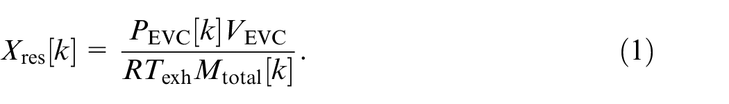
One of the most basic methods applies the ideal gas law to the in-cylinder gases at exhaust valve closing. The state equation requires the in-cylinder pressure ( $P$ ), volume ( $V$ ), and temperature ( $T$ ) in order to calculate the in-cylinder residual mass at EVC. It is also assumed that there is no valve overlap. Since the in-cylinder temperature cannot be directly measured, it has been substituted by the exhaust manifold temperature $T_{\mathrm{exh}}$ . ¹⁷ It is assumed that the in-cylinder volume at EVC ( $V_{\mathrm{EVC}}$ ) is known and constant for all cycles. Therefore, the main source of CCV for the residual gas estimation is the cycle-to-cycle measurement of in-cylinder pressure at EVC. The residual gas fraction is then calculated as follows:

$$X_{\mathrm{res}}[k]=\frac{P_{\mathrm{EVC}}[k]V_{\mathrm{EVC}}}{R{T}_{\mathrm{exh}}{M}_{\mathrm{total}}[k]}.$$

(1)

Here, $R=287$ [J/kgK] is the ideal gas constant for dry air and $M_{\mathrm{total}}[k]$ is the total in-cylinder mass at cycle $k$ , which can be calculated using the model proposed by Daw et al. ⁹ explained in the Appendix. Such a model describes the dynamic coupling between combustion cycles using the carryover of residual gas from the previous cycle to the next. In addition to the residual gas fraction, finding the combustion efficiency is necessary to estimate the total in-cylinder mass; this can be estimated from the gross heat release analysis. Therefore, the equations for residual gas fraction estimation (equation (1)), combustion dynamics (Appendix), and heat release analysis (Appendix) need to be solved simultaneously at each combustion cycle $k$ .

Ideal cycle analysis

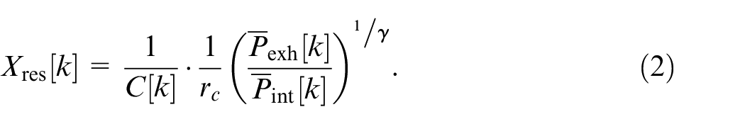
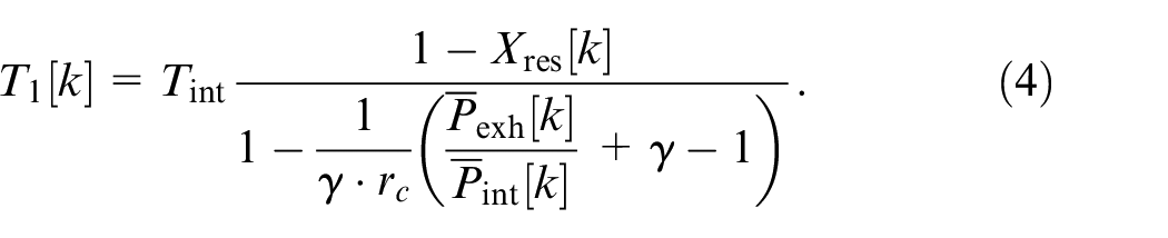
The analysis of a steady-state, constant-volume combustion cycle with an ideal gas performed by Heywood results in the following calculation for the residual gas fraction ⁶ :

$$X_{\mathrm{res}}[k]=\frac{1}{C[k]}·\frac{1}{r_c}{\left(\frac{{\overline{P}}_{\mathrm{exh}}[k]}{{\overline{P}}_{\mathrm{int}}[k]}\right)}^{1/\gamma }.$$

(2)

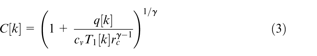
Here, $r_c$ denotes the compression ratio, ${\overline{P}}_{\mathrm{int}}[k]$ and ${\overline{P}}_{\mathrm{exh}}[k]$ denote the average intake and exhaust manifold pressures respectively for each cycle $k$ , $\gamma =1.32$ is the heat capacity ratio calculated during the expansion stroke (before EVO), and the coefficient $C[k]$ is calculated as follows:

$$C[k]={(1+\frac{q[k]}{c_v{T}_1[k]r_c^{\gamma -1}})}^{1/\gamma }$$

(3)

where $c_v=R/(\gamma -1)$ is the specific heat at constant volume and $q[k]$ is the specific energy released during the combustion cycle $k$ . The temperature after adiabatic mixing of the fresh charge and the residual gas is calculated as a function of the intake temperature $T_{\mathrm{int}}$ :

$$T_1[k]=T_{\mathrm{int}}\frac{1-X_{\mathrm{res}}[k]}{1-\frac{1}{\gamma ·r_c}\left(\frac{{\overline{P}}_{\mathrm{exh}}[k]}{{\overline{P}}_{\mathrm{int}}[k]}+\gamma -1\right)}.$$

(4)

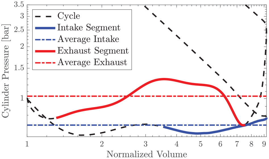
These equations can be solved iteratively given an initial guess for $X_{\mathrm{res}}[k]$ . Figure 1 shows the pressure-volume plot (black dashed line) of a particular experimental cycle $k$ during the intake and exhaust strokes. The segments of the in-cylinder pressure selected to calculate ${\overline{P}}_{\mathrm{int}}[k]$ and ${\overline{P}}_{\mathrm{exh}}[k]$ are highlighted with solid blue and red lines, respectively. The intake segment comprises the crank angle domain between the fuel injection ( $-300$ [CA deg]) and bottom dead center (BDC). The exhaust segment was selected after blowdown ( $240$ [CA deg]) and before intake valve opening. The values of ${\overline{P}}_{\mathrm{int}}[k]$ and ${\overline{P}}_{\mathrm{exh}}[k]$ were calculated by averaging the pressure over the aforementioned segments, and they are depicted in dash-dotted lines in Figure 1. This approach provides the first source of CCV for the residual fraction estimation.

Figure 1.

Pressure-Volume plot (black dashed line) during the gas exchange process. Segments used to calculate average intake ( ${\overline{P}}_{\mathrm{int}}$ ) and exhaust ( ${\overline{P}}_{\mathrm{exh}}$ ) pressures are highlighted with solid blue and red lines, respectively. Dash-dotted lines show the values of ${\overline{P}}_{\mathrm{int}}[k]$ and ${\overline{P}}_{\mathrm{exh}}[k]$ for the current cycle.

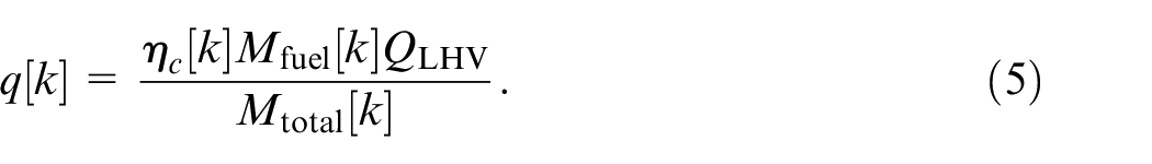
Another source of CCV comes from the combustion part. Consider calculating the specific energy release at each cycle $k$ as follows:

$$q[k]=\frac{{\eta }_c[k]M_{\mathrm{fuel}}[k]Q_{\mathrm{LHV}}}{M_{\mathrm{total}}[k]}.$$

(5)

Here, $Q_{\mathrm{LHV}}=41$ [MJ/kg] is the lower heating value of the fuel. The combustion efficiency ${\eta }_c$ can be calculated from the gross heat release analysis described in the Appendix. Under the ideal cycle assumption, the factor $C[k]$ defined in equation (3) is an increasing function of the specific energy release. Let $q_{\max }$ be the maximum specific energy release, which generates the maximum $C_{\max }$ . Note that a misfire event results in $q_{\min }=0\Rightarrow C_{\min }=1$ . Therefore, for any cycle $k$ , the factor $C$ satisfies $1⩽C[k]⩽C_{\max }$ . Since the residual fraction is inverse proportional to $C[k]$ , then $X_{\mathrm{res}}[k]$ reaches its maximum in the same cycle where a misfire occurs. Correspondingly, the residual fraction achieves its minimum at $q_{\max }$ .

Ideal cycle analysis with valve overlap

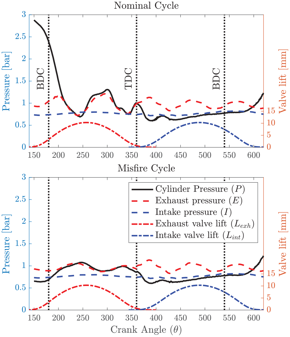
The method previously discussed for estimating the residual gas fraction assumes no valve overlap (VO). However, the experimental engine campaign presented in this study presents a valve overlap of 55 [CA deg]. The ideal cycle analysis can be extended to include the effects of the overlap, as demonstrated by Cavina et al. ¹⁶ In this case, the residual gas fraction is not only the result of the trapped mass before intake valve opening (IVO) but also includes the contribution of the backflow from the exhaust manifold when both valves are open. Such a backflow is driven by the pressure difference between the intake and exhaust manifolds during the valve overlap. In order to accurately capture this pressure difference, high-speed intake and exhaust manifold pressure sensors were utilized. Figure 2 shows in dashed lines the measurements of such high-speed sensors. The black solid line shows the in-cylinder pressure, while the dash-dotted lines represent intake and exhaust valves lift profiles. Note that the gas exchange process is different between nominal combustion events (top plot) and misfire events (bottom plot). Such a difference can be captured by the high-speed intake and exhaust sensor measurements during valve overlap.

Figure 2.

Valve overlap event after a nominal (top) and after a misfire cycle (bottom). Black solid line represents in-cylinder pressure, dashed lines represent high-speed manifold pressure sensors, dash-dotted lines represent valve lift profiles.

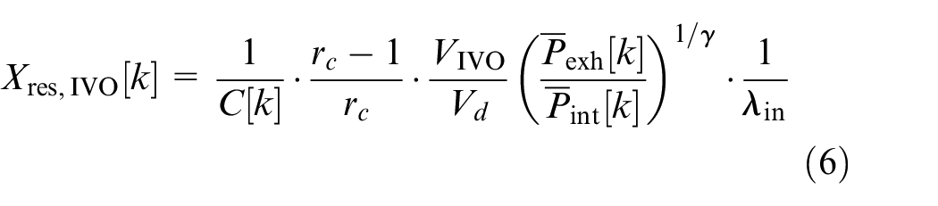
According to Cavina et al., the trapped residual gas at IVO can be calculated in a similar fashion as equation (2):

$$X_{\mathrm{res},\mathrm{IVO}}[k]=\frac{1}{C[k]}·\frac{r_c-1}{r_c}·\frac{V_{\mathrm{IVO}}}{V_d}{\left(\frac{{\overline{P}}_{\mathrm{exh}}[k]}{{\overline{P}}_{\mathrm{int}}[k]}\right)}^{1/\gamma }·\frac{1}{{\lambda }_{\mathrm{in}}}$$

(6)

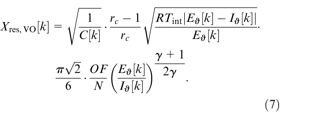
where $V_d$ is the displacement volume, $V_{\mathrm{IVO}}$ is the in-cylinder volume at IVO, and ${\lambda }_{\mathrm{in}}=1$ is the air-fuel equivalence ratio of the fresh charge. The factor $C[k]$ is calculated using equation (3). Let $\vartheta =370$ [CAD] be the crank angle location where the intake and exhaust valves have the same lift during the overlap. Define $I_{\vartheta }[k]$ and $E_{\vartheta }[k]$ as the intake and exhaust manifold pressures, respectively, recorded by the high-speed sensors at the crank angle $\vartheta$ for cycle $k$ . Note in Figure 2 the inequality $I_{\vartheta }[k]<E_{\vartheta }[k]$ holds, which produces the backflow of gases into the cylinder and increases the residual gas. The residual gas due to the backflow of gasses from the exhaust manifold into the cylinder is:

$$\begin{array}{c}{X}_{\mathrm{res},\mathrm{VO}}[k]=\sqrt{\frac{1}{C[k]}}·\frac{r_c-1}{r_c}\sqrt{\frac{R{T}_{\mathrm{int}}|E_{\vartheta }[k]-I_{\vartheta }[k]|}{E_{\vartheta }[k]}}·\hfill \\ \frac{\pi \sqrt{2}}{6}·\frac{\mathrm{OF}}{N}{\left(\frac{E_{\vartheta }[k]}{I_{\vartheta }[k]}\right)}^{\frac{\gamma +1}{2\gamma }}.\hfill \end{array}$$

(7)

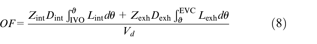
Here, $N$ is the engine speed and $\mathrm{OF}$ is the overlap factor calculated as follows:

$$\mathrm{OF}=\frac{Z_{\mathrm{int}}{D}_{\mathrm{int}}{\int }_{\mathrm{IVO}}^{\vartheta }{L}_{\mathrm{int}}d\theta +Z_{\mathrm{exh}}{D}_{\mathrm{exh}}{\int }_{\vartheta }^{\mathrm{EVC}}{L}_{\mathrm{exh}}d\theta }{V_d}$$

(8)

where $L$ is the valve lift, $D$ is the valve inner seat diameter, and $Z$ is the number of valves. Finally, the residual gas fraction at each cycle is calculated as

$$X_{\mathrm{res}}[k]=X_{\mathrm{res},\mathrm{IVO}}[k]+X_{\mathrm{res},\mathrm{VO}}[k].$$

(9)

Note that this method can provide high accuracy in a multi-cylinder environment where additional backflow dynamics are present due to the pumping flow characteristics of the other cylinders. However, this would also require additional sensors for each intake/exhaust runners, increasing instrumentation complexity and cost.

Isentropic expansion (Mirsky method)

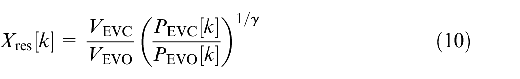
Yun and Mirsky showed that the residual gas fraction can be estimated under the assumptions of an ideal gas, isentropic exhaust process between EVO and EVC, and no valve overlap. ¹⁸ This results in the following calculation:

$$X_{\mathrm{res}}[k]=\frac{V_{\mathrm{EVC}}}{V_{\mathrm{EVO}}}{\left(\frac{P_{\mathrm{EVC}}[k]}{P_{\mathrm{EVO}}[k]}\right)}^{1/\gamma }$$

(10)

which depends solely on the conditions at EVO and EVC. In general, $P_{\mathrm{EVC}}$ behaves similar to a Gaussian random variable with a mean value approximately equal to the exhaust manifold pressure. This implies that $P_{\mathrm{EVC}}$ is mostly independent from the cycle-to-cycle combustion events. On the other hand, the in-cylinder pressure at EVO presents significant changes depending on the levels of energy released at each cycle. Note that, different from the methods involving ideal cycle assumptions, equation (10) can be calculated without relying on solving the combustion dynamics or the gross heat release. Hence, it presents an advantage for real-time implementation.

Fitzgerald method

The ideal cycle analysis assumes a steady-state, adiabatic, and reversible combustion cycle. Fitzgerald et al. analyzed the exhaust process from EVO to EVC assuming an ideal gas undergoing a reversible process but including heat loss. ¹⁹ Consider dividing the exhaust process into two stages:

1. Blowdown: In-cylinder pressure reduces from $P_{\mathrm{EVO}}$ to the exhaust manifold pressure.

2. Recompression: Residual gases undergo polytropic recompression after blowdown as the piston moves upwards to TDC.

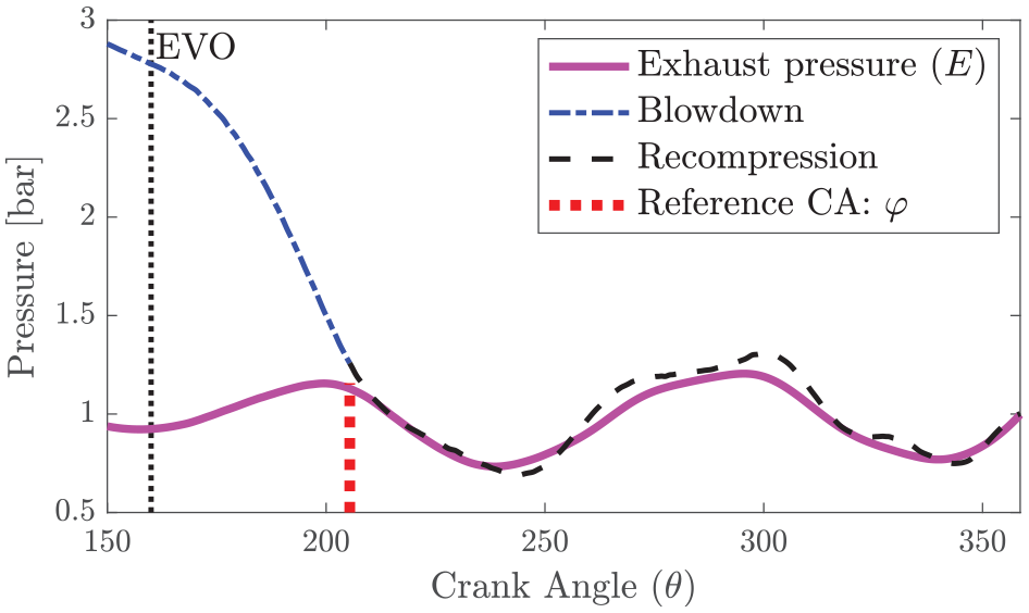
Figure 3 shows the in-cylinder pressure and the exhaust manifold pressure recorded by the high-speed sensor during the exhaust process. Let $\phi$ be the crank angle at the end of the blowdown stage and the beginning of the recompression stage. Note that $\phi [k]$ is affected by CCV and needs to be calculated at each cycle $k$ . Nonetheless, such an angle demonstrated low variability with a mean value of $\mathbb{E}[\phi ]=205$ [CA deg].

Figure 3.

Blowdown and recompression stages during exhaust process for Fitzgerald method.

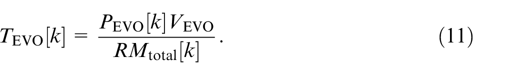
At the start of the exhaust process, the temperature at EVO can be calculated from the ideal gas law and knowledge of the in-cylinder gas composition:

$$T_{\mathrm{EVO}}[k]=\frac{P_{\mathrm{EVO}}[k]V_{\mathrm{EVO}}}{R{M}_{\mathrm{total}}[k]}.$$

(11)

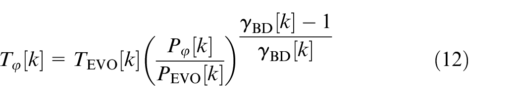
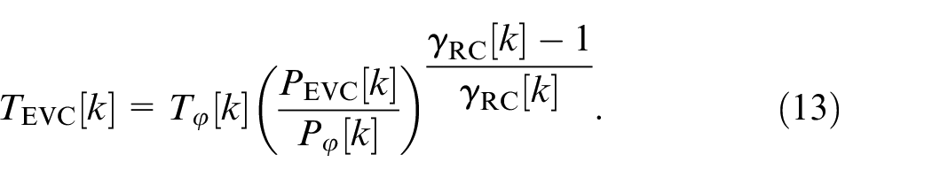
During each stage of the exhaust process, it is assumed that the residual gas undergoes a polytropic process with a distinct polytropic coefficient, then:

$$T_{\phi }[k]=T_{\mathrm{EVO}}[k]{\left(\frac{P_{\phi }[k]}{P_{\mathrm{EVO}}[k]}\right)}^{\frac{{\gamma }_{\mathrm{BD}}[k]-1}{{\gamma }_{\mathrm{BD}}[k]}}$$

(12)

$$T_{\mathrm{EVC}}[k]=T_{\phi }[k]{\left(\frac{P_{\mathrm{EVC}}[k]}{P_{\phi }[k]}\right)}^{\frac{{\gamma }_{\mathrm{RC}}[k]-1}{{\gamma }_{\mathrm{RC}}[k]}}.$$

(13)

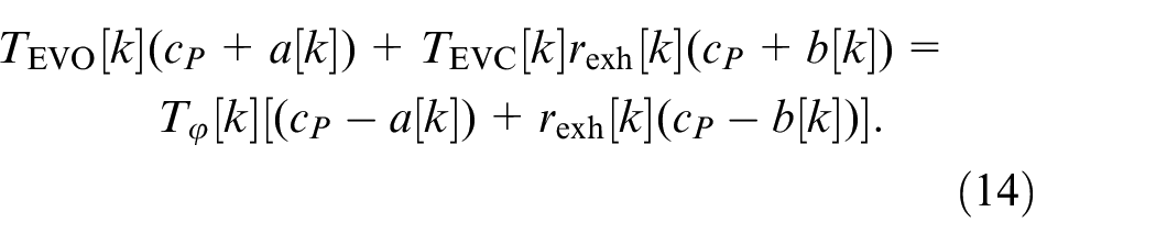
The analysis done by Fitzgerald et al., summarized in the Appendix, provides equation (A12) which relates the temperatures during the exhaust process ( $T_{\mathrm{EVO}},T_{\phi },T_{\mathrm{EVC}}$ ) as follows:

$$\begin{array}{c}{T}_{\mathrm{EVO}}[k](c_P+a[k])+T_{\mathrm{EVC}}[k]r_{\mathrm{exh}}[k](c_P+b[k])=\hfill \\ T_{\phi }[k][(c_P-a[k])+r_{\mathrm{exh}}[k](c_P-b[k])].\hfill \end{array}$$

(14)

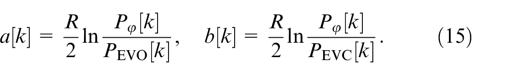
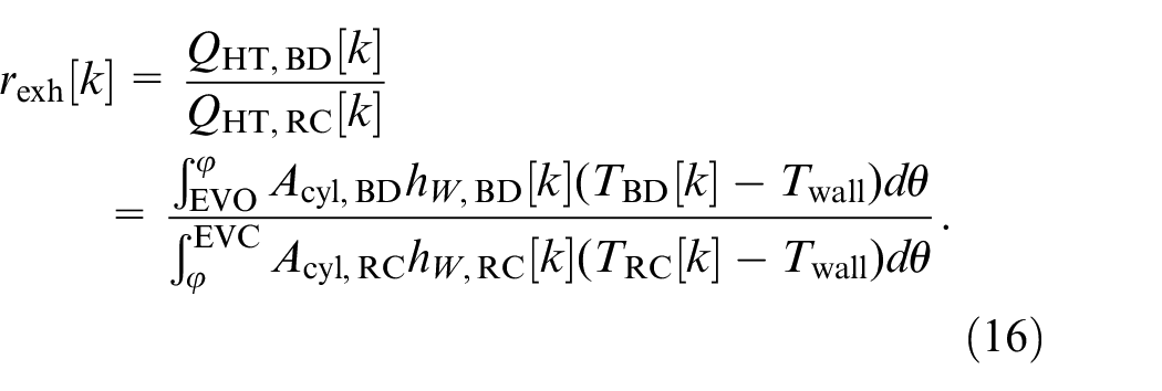
Here, $c_P$ is the specific heat at constant pressure, $r_{\mathrm{exh}}[k]$ is the ratio between the heat loss during blowdown and the heat loss during recompression, and the values $a[k]$ and $b[k]$ are calculated at each cycle as follows:

$$a[k]=\frac{R}{2}\mathrm{In}\frac{P_{\phi }[k]}{P_{\mathrm{EVO}}[k]},b[k]=\frac{R}{2}\mathrm{In}\frac{P_{\phi }[k]}{P_{\mathrm{EVC}}[k]}.$$

(15)

In this study, we assumed constant values for $R$ and $c_P=R·\gamma /(\gamma -1)$ . The final equation comes from the definition of the heat loss ratio, which can be calculated using the convective heat transfer from the in-cylinder gases to the cylinder wall:

$$\begin{array}{c}{r}_{\mathrm{exh}}[k]=\frac{Q_{\mathrm{HT},\mathrm{BD}}[k]}{Q_{\mathrm{HT},\mathrm{RC}}[k]}\hfill \\ =\frac{{\int }_{\mathrm{EVO}}^{\phi }{A}_{\mathrm{cyl},\mathrm{BD}}{h}_{W,\mathrm{BD}}[k](T_{\mathrm{BD}}[k]-T_{\mathrm{wall}})d\theta }{{\int }_{\phi }^{\mathrm{EVC}}{A}_{\mathrm{cyl},\mathrm{RC}}{h}_{W,\mathrm{RC}}[k](T_{\mathrm{RC}}[k]-T_{\mathrm{wall}})d\theta }.\hfill \end{array}$$

(16)

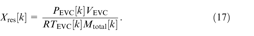
Here, $A_{\mathrm{cyl}}$ represents the cylinder surface area and $h_W$ is the Woschni’s heat transfer coefficient, calculated using equation (A6) in the Appendix. Note that $T_{\mathrm{BD}}[k]$ and $T_{\mathrm{RC}}[k]$ can be calculated using the polytropic equations (12) and (13), respectively. Therefore, assuming knowledge of $T_{\mathrm{EVO}}$ , equations (12), (13), (14), and (16) represent a system of four equations with five unknows: $T_{\phi }$ , $T_{\mathrm{EVC}}$ , ${\gamma }_{\mathrm{BD}}$ , ${\gamma }_{\mathrm{RC}}$ , and $r_{\mathrm{exh}}$ . In the original study, Fitzgerald et al. related $T_{\phi }$ to the exhaust manifold temperature using the simple linear equation: $T_{\phi }=T_{\mathrm{exh}}+\mathrm{\Delta }T$ , where $\mathrm{\Delta }T$ was calibrated from a high-fidelity GT-Power model. In the absence of such a calibration procedure, consider using a constant and known polytropic coefficient, either ${\gamma }_{\mathrm{BD}}$ or ${\gamma }_{\mathrm{RC}}$ , equal to the isentropic coefficient $\gamma =1.32$ . The resulting system of equations can be solved iteratively providing the initial guess $r_{\mathrm{exh},\mathrm{init}}[k]=1$ . Finally, after the solution is found, the residual gas fraction can be calculated utilizing the state equation at EVC as follows:

$$X_{\mathrm{res}}[k]=\frac{P_{\mathrm{EVC}}[k]V_{\mathrm{EVC}}}{R{T}_{\mathrm{EVC}}[k]M_{\mathrm{total}}[k]}.$$

(17)

One can show, however, that if ${\gamma }_{\mathrm{BD}}[k]={\gamma }_{\mathrm{RC}}[k]$ then the solution simplifies to the one provided by the isentropic method in equation (10).

Control-oriented modeling

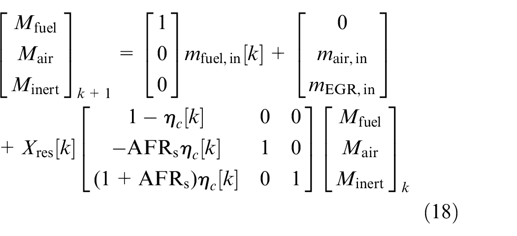
Given that this study focuses on the application of different residual gas estimation methods for next-cycle control of combustion CCV, consider evaluating their ability to provide an accurate control-oriented model. The physics-based approached considering composition changes from prior cycles (discussed in the Appendix) can be summarized by the following dynamic system ⁹ :

$$\begin{array}{c}{\left[\begin{array}{c}{M}_{\mathrm{fuel}}\hfill \\ \multicolumn{1}{c}{M_{\mathrm{air}}}\\ \multicolumn{1}{c}{M_{\mathrm{inert}}}\end{array}\right]}_{k+1}=\left[\begin{array}{c}1\hfill \\ \multicolumn{1}{c}{0}\\ \multicolumn{1}{c}{0}\end{array}\right]m_{\mathrm{fuel},\mathrm{in}}[k]+\left[\begin{array}{c}0\hfill \\ \multicolumn{1}{c}{m_{\mathrm{air},\mathrm{in}}}\\ \multicolumn{1}{c}{m_{\mathrm{EGR},\mathrm{in}}}\end{array}\right]\hfill \\ +X_{\mathrm{res}}[k]\left[\begin{array}{ccc}1-{\eta }_c[k]\hfill & 0\hfill & 0\hfill \\ \multicolumn{1}{c}{-\mathrm{AF}{\mathrm{R}}_{\mathrm{s}}{\eta }_c[k]}& 1\hfill & 0\hfill \\ \multicolumn{1}{c}{(1+\mathrm{AF}{\mathrm{R}}_{\mathrm{s}}){\eta }_c[k]}& 0\hfill & 1\hfill \end{array}\right]{\left[\begin{array}{c}{M}_{\mathrm{fuel}}\hfill \\ \multicolumn{1}{c}{M_{\mathrm{air}}}\\ \multicolumn{1}{c}{M_{\mathrm{inert}}}\end{array}\right]}_k\hfill \end{array}$$

(18)

$$Q_{\mathrm{gross}}[k]={\eta }_c[k]M_{\mathrm{fuel}}[k]Q_{\mathrm{LHV}}.$$

(19)

Equation (18) corresponds to the system dynamics. Here $\mathrm{AF}{\mathrm{R}}_s$ is the stoichiometric air-to-fuel ratio (AFR), $m_{\mathrm{fuel},\mathrm{in}}$ is the mass of fuel injected during the intake stroke, considered as the control variable, $m_{\mathrm{air},\mathrm{in}}$ and $m_{\mathrm{EGR},\mathrm{in}}$ are the masses of fresh air and EGR admitted into the cylinder, and $M_{\mathrm{fuel}},M_{\mathrm{air}},M_{\mathrm{inert}}$ are the total amount of in-cylinder fuel, air, and inert gas. Equation (19) corresponds to the observation or output of the system. Therefore, at any cycle $k$ , the states of the system are the total in-cylinder masses of fuel $M_{\mathrm{fuel}}[k]$ , air $M_{\mathrm{air}}[k]$ , and burned gas $M_{\mathrm{inert}}[k]$ . The gross heat release $Q_{\mathrm{gross}}[k]$ is the measured output and was considered as the proxy variable for characterizing combustion CCV.

Note that the model intrinsically considers the engine speed and engine load, which determines the volumetric efficiency ( $m_{\mathrm{air},\mathrm{in}}$ and $m_{\mathrm{EGR},\mathrm{in}}$ ) of the cylinder. Geometric properties of the combustion chamber are condensed in the combustion efficiency ${\eta }_c$ , which depends on heat transfer characteristics. Temperature and ambient conditions, as well as speed and load, are all captured in both ${\eta }_c$ and $X_{\mathrm{res}}$ . However, since such parameters vary in a cycle-to-cycle basis, offline simulation depends on empirical functions for ${\eta }_c$ and $X_{\mathrm{res}}$ extracted from data. This constraints the offline simulations to a single speed/load condition.

In order to perform offline simulations, the model parameters $X_{\mathrm{res}}[k]$ and ${\eta }_c[k]$ need to be functions of the states. Instead of tracking all three states, consider defining the gas-fuel equivalence ratio:

$$\lambda \prime [k]=\frac{M_{\mathrm{air}}[k]+M_{\mathrm{inert}}[k]}{M_{\mathrm{fuel}}[k]}·\frac{1}{\mathrm{AF}{\mathrm{R}}_s}.$$

(20)

The gas-fuel equivalence ratio was used as an indicator of the ignition limit under high dilution of burned gases. ²² The model assumes that, at any cycle $k$ , the combustion efficiency is a sigmoidal function of $\lambda \prime [k]$ :

$${\eta }_c[k]={\eta }_c^{*}\frac{1}{1+{100}^{\frac{\lambda \prime [k]-{\mu }_{\lambda \prime }}{{\mathrm{\Delta }}_{\lambda \prime }}}}(1+\mathrm{Co}{\mathrm{V}}_Q·w[k])$$

(21)

where ${\eta }_c^{*}=0.95$ is the measured combustion efficiency and the parameters ${\mu }_{\lambda \prime }$ and ${\mathrm{\Delta }}_{\lambda \prime }$ need to be calibrated. The parameter $\mathrm{Co}{\mathrm{V}}_Q=2\%$ is the coefficient of variability for the nominal values of $Q_{\mathrm{gross}}$ , assumed to be constant, and $\{w[k]{\}}_{k\in \mathbb{N}}$ is a sequence of uncorrelated standard Gaussian random variables. The original hypothesis of the study by Daw et al. considered a constant value for the residual gas fraction with Gaussian white noise superimposed. However, a more recent analysis presented by the authors assumes a strong correlation with the gross heat release ²³ :

$$X_{\mathrm{res}}[k]=f_X(Q_{\mathrm{gross}}[k])+{\sigma }_X·v[k].$$

(22)

The function $f_X(·)$ was found using a fifth-order polynomial regression assuming that the random perturbation $v[k]$ is Gaussian white noise. The parameter ${\sigma }_X$ can be calculated from the distribution of the residuals from the regression of $f_X(·)$ .

Results and discussion

The current section presents the results of the different estimation methods utilizing a common experimental data set of 5000 consecutive engine cycles. Based on the modeling approach, three variables where chosen for analysis: (1) the gas-fuel equivalence ratio, (2) the combustion efficiency, and (3) the residual gas fraction. In addition, the gross heat release is also considered in order to evaluate cycle-to-cycle dynamics. For time series plots, a common window of 60 cycles was chosen to study the cycle-to-cycle behavior of such variables.

State equation

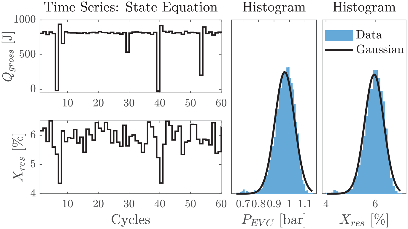
Figure 4 shows the results of the estimation. The left plots show the time series of the gross heat release and residual gas fraction during a 60 cycles window. Even though the CCV induced by sporadic partial burns and misfires is captured by $Q_{\mathrm{gross}}$ , the estimation of $X_{\mathrm{res}}$ shows a Gaussian distribution centered at a mean value of $\mathbb{E}[X_{\mathrm{res}}]=6$ [%]. The probability distribution of $X_{\mathrm{res}}$ (right plot) is a direct consequence of the randomness of the measured $P_{\mathrm{EVC}}$ , which has a mean value close to the exhaust manifold pressure (center plot). The time series of $X_{\mathrm{res}}$ shows mostly a random behavior except when a misfire occurs, which produces a lower-than-nominal residual fraction at cycle $k$ followed by the minimum value at cycle $k+1$ . This behavior contributes to the heavy lower tail of the residual gas fraction distribution. Even though this estimation method suggests that $X_{\mathrm{res}}[k]$ can be modeled by a constant value with additive Gaussian random perturbations, the remaining estimation methods provide a better insight on the relationship between cycle-to-cycle energy release and residual gas fraction.

Figure 4.

Time series of gross heat release and estimated residual gas fraction (left), histograms of in-cylinder pressure at EVC (center) and residual gas fraction estimate (right).

Ideal cycle analysis

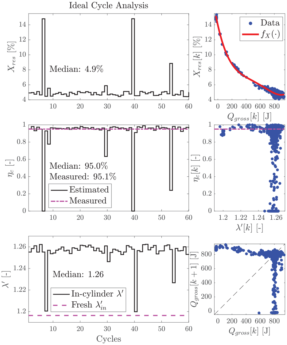
Figure 5 shows the results of the residual gas fraction estimation using the ideal cycle analysis. The left column shows the time series of the three main model parameters. When a misfire event occurs, the combustion efficiency drops to zero. As previously discussed, the residual gas fraction achieves its maximum value during the misfire. In the cycle following the misfire event, the residual gas composition (in absence of combustion) is similar to the fresh gas composition admitted into the cylinder. In general, the in-cylinder gas-fuel equivalence ratio $\lambda \prime [k]$ is higher than the equivalence ratio of the fresh charge ${\lambda }_{\mathrm{in}}^{\prime }=(m_{\mathrm{air},\mathrm{in}}+m_{\mathrm{EGR},\mathrm{in}})/m_{\mathrm{fuel},\mathrm{in}}·1/{\mathrm{AFR}}_s$ due to the burned residual gas. Therefore, after a misfire, the in-cylinder gas-fuel equivalence ratio decreases toward ${\lambda }_{\mathrm{in}}^{\prime }$ . The excess of residual unburned fuel in the successive cycle generates a high energy release, where $Q_{\mathrm{gross}}$ achieves its maximum. Such a deterministic behavior (high energy release after a misfire) has been observed by the authors in previous studies and can be observed in the asymmetry of the return map for $Q_{\mathrm{gross}}$ (bottom right plot).^10,24,25

Figure 5.

Time series of model parameters (left) and functional relationships (right) obtained using the ideal cycle analysis as the residual gas fraction estimation method.

The functional relationship $X_{\mathrm{res}}[k]=f_X(Q_{\mathrm{gross}}[k])$ is shown in the top right plot for all 5000 experimental cycles. The residual fraction can be predicted by a non-increasing polynomial function of $Q_{\mathrm{gross}}$ (solid red line). However, note that the function flattens for values of $Q_{\mathrm{gross}}>800$ [J], indicating that nominal and high-energy cycles produce similar residual fraction estimates. This relationship contradicts the previous result using the state equation, where the estimated residual fraction remained mostly constant regardless of the energy release. The relationship between the combustion efficiency and gas-fuel equivalence ratio is depicted in the middle right plot. Note that the values of ${\eta }_c$ remain fairly constant until the gas composition reaches the ignition limit $\lambda \prime \approx 1.26$ . At this point, a sharp drop in combustion efficiency occurs which causes misfires and partial burns. Such a sudden change was modeled using the sigmoid function in equation (21).

Ideal cycle analysis with valve overlap

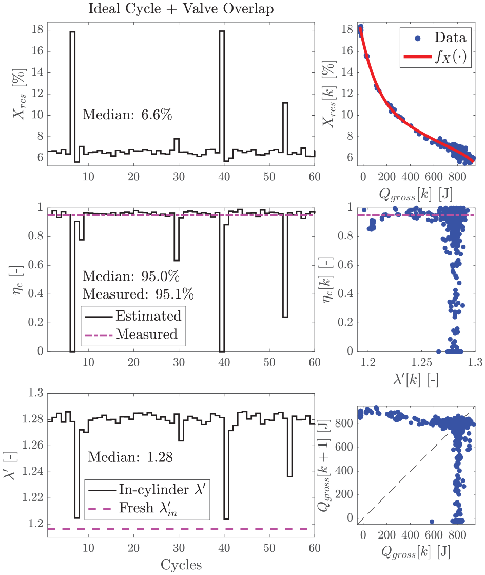
Figure 6 shows the results for the residual gas fraction estimation algorithm using the ideal cycle analysis with valve overlap. As expected, the nominal value of the estimated residual gas fraction increases when valve overlap is considered. Even though the methodology is similar to the one discussed for the ideal cycle analysis, two important differences arise. Although the residual gas fraction achieves its maximum at the misfire, the successive cycle shows a lower-than-nominal value (top-right figure). As previously observed, the cycle succeeding a misfire presents a gas-fuel equivalence ratio value closer to the admitted gas composition ${\lambda }_{\mathrm{in}}^{\prime }$ . In addition, we can observe that $\lambda \prime [k]$ does not return to the nominal value immediately after the gas-fuel equivalence ratio achieves its minimum. Note that $\lambda \prime [k]$ follows a first-order response after the perturbation caused by the misfire, taking longer than one cycle to reach the nominal value. The overall values and dynamic response of ${\eta }_c$ and $Q_{\mathrm{gross}}$ are very similar to those shown in Figure 5. The functional dependencies showed in the right column present similar trends to the ones discussed in the previous method. The top-right plot, however, presents slight differences compared with the previous results. In this case, $X_{\mathrm{res}}[k]$ can be described by a strictly decreasing function of $Q_{\mathrm{gross}}[k]$ . This means that high-energy cycles produce a lower residual fraction than nominal cycles. Although the ignition limit changes due to the higher residual fraction estimate, the sharp decrease in combustion efficiency is still observed. For low values of $\lambda \prime$ , however, a slight decrease in combustion efficiency is observed.

Figure 6.

Time series of model parameters (left) and functional relationships (right) obtained using the ideal cycle analysis with valve overlap as the residual gas fraction estimation method.

Isentropic expansion (Mirsky method)

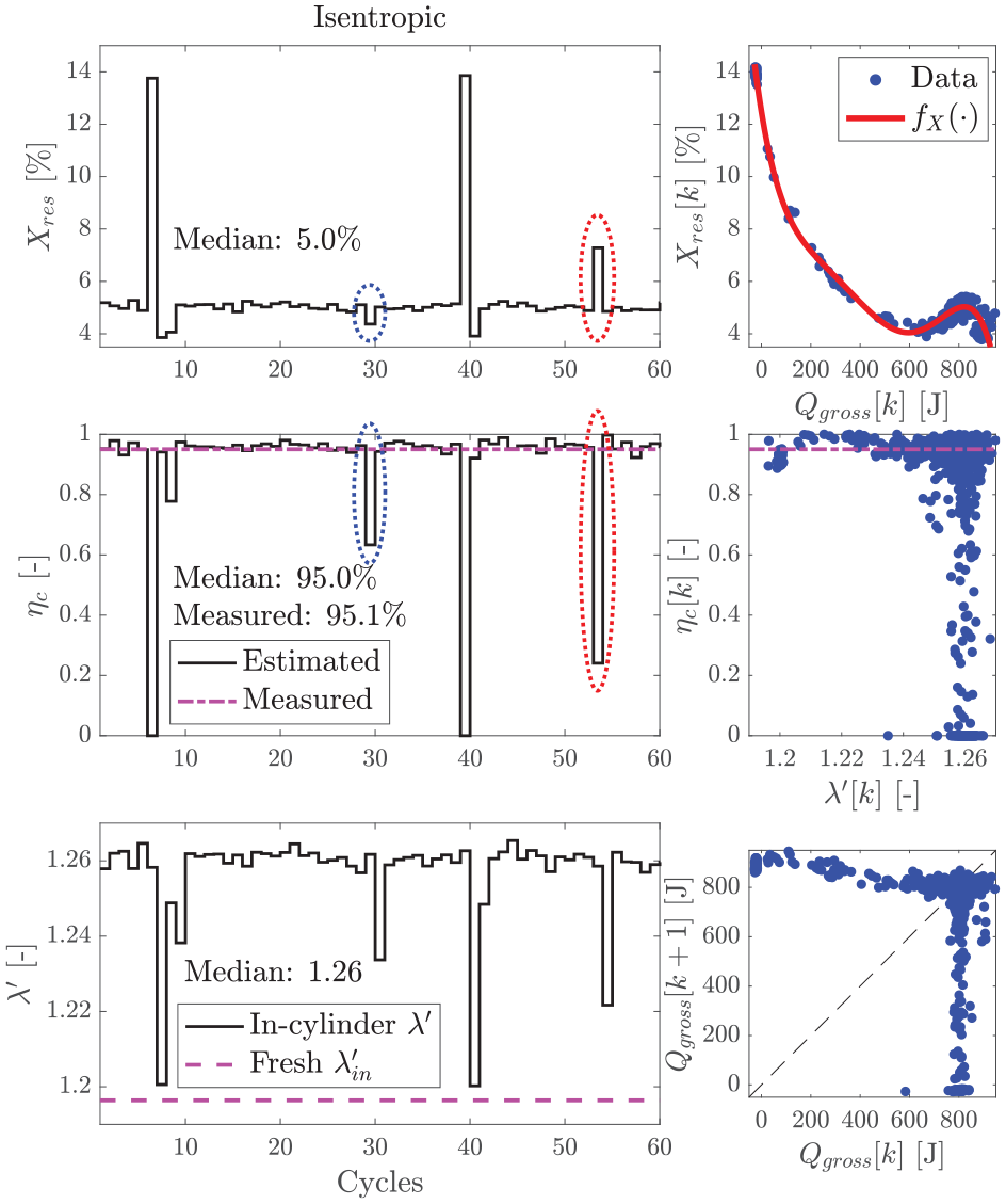
Figure 7 shows the results when using the isentropic assumption. Note that the nominal value of $X_{\mathrm{res}}$ agrees closely with the value obtained using the ideal cycle analysis without valve overlap. However, the relationship between energy release and the residual fraction is no longer monotonic. The top-right plot shows a monotonically increasing trend of $X_{\mathrm{res}}$ for $550⩽Q_{\mathrm{gross}}⩽820$ , while maintaining a strictly decreasing relationship for the rest of the domain. This non-monotonic behavior can also be seen in the time series of $X_{\mathrm{res}}$ . The blue ellipse highlights the residual fraction estimation for a cycle in which the energy release falls between the interval $550⩽Q_{\mathrm{gross}}⩽820$ . Such an estimate is lower than the nominal value for $X_{\mathrm{res}}$ , which has the opposite trend compared to the previous estimates calculated using ideal cycle assumptions. The red ellipse highlights a cycle with $Q_{\mathrm{gross}}<550$ which presents a residual estimate significantly higher than the nominal value. Despite this opposite behavior, the combustion efficiency and gross heat release estimates follow a similar trend as previously found. The plot ${\eta }_c[k]$ vs. $\lambda \prime [k]$ , however, shows combustion efficiency values closer to one for $1.21⩽\lambda \prime ⩽1.23$ , which previous methods estimated values closer to nominal. Similar to the ideal cycle analysis with valve overlap, the gas-fuel equivalence ratio achieves the value similar to the fresh ${\lambda }_{\mathrm{in}}^{\prime }$ in the cycle after a misfire, but it does not go back to the nominal value in the subsequent cycle. In general, it takes two cycles after the misfire to reach the nominal value of $\lambda \prime$ . The bottom-right plot shows that the dynamic behavior and the absolute value of the gross heat release is fairly similar for the ideal, valve overlap, and isentropic methods.

Figure 7.

Time series of model parameters (left) and functional relationships (right) obtained using the isentropic assumption as the residual gas fraction estimation method.

Fitzgerald method

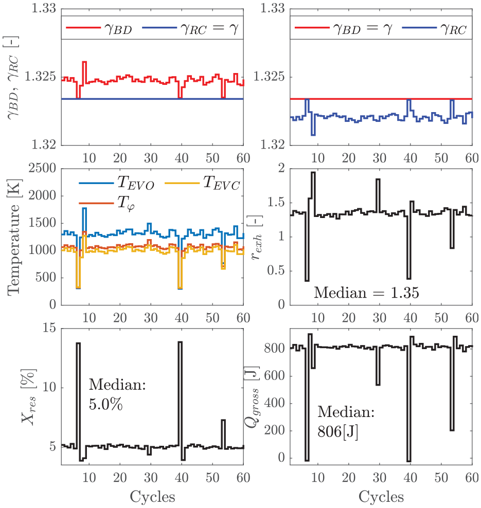
Recall that, in order to solve the system of equations outlined by the Fitzgerald method, it was assumed that one polytropic coefficient is constant and known. The top row of Figure 8 shows the resulting values for polytropic coefficients either assuming that ${\gamma }_{\mathrm{RC}}[k]=\gamma$ (left) or that ${\gamma }_{\mathrm{BD}}[k]=\gamma$ (right). For either set of assumptions, note that the inequality ${\gamma }_{\mathrm{RC}}[k]⩽{\gamma }_{\mathrm{BD}}[k]$ always holds, which agrees with the observations of Fitzgerald et al. Also note that during a misfire ${\gamma }_{\mathrm{BD}}[k]\approx {\gamma }_{\mathrm{RC}}[k]$ , which shows that the blowdown and recompression phases have similar rates of heat loss and similar temperatures throughout the exhaust process. Even though CCV is present in the estimates of either ${\gamma }_{\mathrm{BD}}$ or ${\gamma }_{\mathrm{RC}}$ , on average, the difference between such values is significantly small: $\mathbb{E}[{\gamma }_{\mathrm{BD}}[k]]-\mathbb{E}[{\gamma }_{\mathrm{RC}}[k]]=0.0014$ for both sets of assumptions. The second row of Figure 8 shows the temperatures during the exhaust process and the heat loss ratio. As expected, we observed that $T_{\mathrm{EVO}}⩾T_{\phi }⩾T_{\mathrm{EVC}}$ during combustion and $T_{\mathrm{EVO}}\approx T_{\phi }\approx T_{\mathrm{EVC}}$ during misfires. The nominal value for the heat loss ratio was $r_{\mathrm{exh}}=1.35$ , which is similar to the values reported by Fitzgerald et al. ¹⁹ and Larimore et al. ²⁶ When combustion is present, $r_{\mathrm{exh}}[k]>1$ since most of the heat loss occurs during blowdown due to the rapid equalization of pressures that enhances convective heat transfer. Even though for misfires the heat loss is almost constant during the exhaust process, $r_{\mathrm{exh}}[k]<1$ because the blowdown period is shorter than the recompression period. The bottom row of Figure 8 shows the resulting estimates for $X_{\mathrm{res}}$ and $Q_{\mathrm{gross}}$ under the assumption that ${\gamma }_{\mathrm{RC}}=\gamma$ . The small difference between the polytropic coefficients during blowdown and recompression generates almost the exact estimates as the isentropic method. A similar conclusion holds when ${\gamma }_{\mathrm{BD}}=\gamma$ is assumed instead. Therefore, the isentropic method will be preferred over the Fitzgerald method for simplicity in its implementation.

Figure 8.

Time series of variables involved in the residual gas fraction estimation using the Fitzgerald method.

Performance comparison

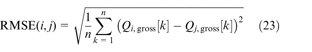
The methods were evaluated specifically in the context of whether they provide estimates that are consistent with observed dynamics of cycle-to-cycle variations in heat release. Based on the control-oriented model presented in equations (18) and (19), the gross heat release was used as the variable for comparing the performance and usefulness of the different estimation methods. In order to compare the differences between all the methods proposed, consider using the root mean square error (RMSE) and the maximum absolute difference (MAD) defined as follows:

$$\mathrm{RMSE}(i,j)=\sqrt{\frac{1}{n}\sum _{k=1}^n{(Q_{i,\mathrm{gross}}[k]-Q_{j,\mathrm{gross}}[k])}^2}$$

(23)

$$\mathrm{MAD}(i,j)=\underset{1⩽k⩽n}{max}|Q_{i,\mathrm{gross}}[k]-Q_{j,\mathrm{gross}}[k]|.$$

(24)

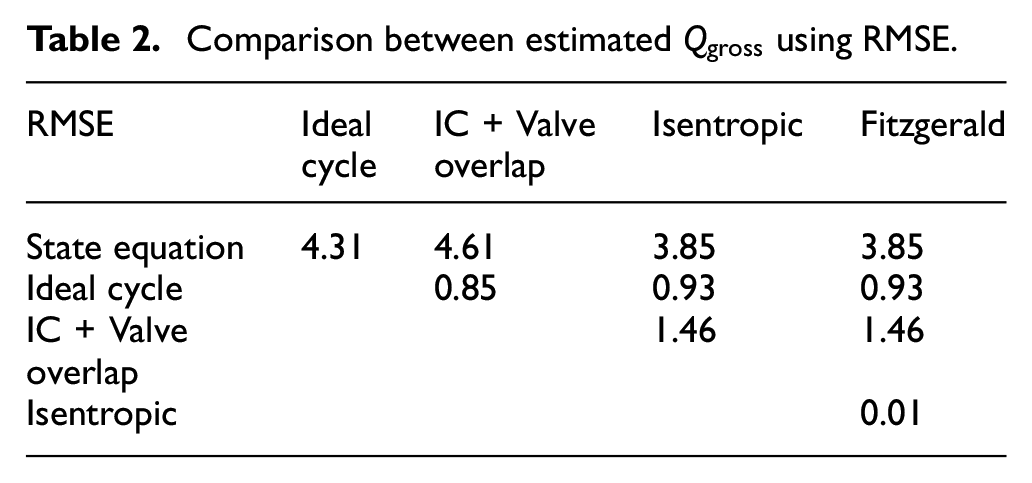
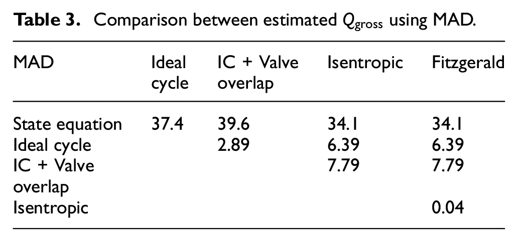
The variable $n=5000$ indicates the total number of experimental combustion cycles recorded and the subscripts $i$ and $j$ represent the different estimation methods. Tables 2 and 3 show the numerical values for RMSE $(i,j)$ and MAD $(i,j)$ . The higher discrepancy is achieved when the state equation method is compared against the rest. Even though the RMSE values correspond to only a 0.6% error, based on the nominal value of $Q_{\mathrm{gross}}=806$ [J], the MAD values are relatively high. The highest discrepancy occurs when estimating high-energy cycles following misfires. During such events, the state equation method overestimates these values by $30$ [J] on average. The remaining estimation methods, however, show a very close agreement in $Q_{\mathrm{gross}}$ estimation with an $\mathrm{RMSE}<1.5$ [J] and $\mathrm{MAD}<8$ [J]. The particularly low value of the RMSE shows that such methods, on average, provide the same estimate. Also note that, as previously discussed, the isentropic and Fitzgerald methods provide practically the same result. Even though these results show that all methods can capture the magnitude of combustion CCV and provide similar cycle-to-cycle values, it is not clear which method can also correctly capture functional dependencies needed for offline simulation.

Table 2.

Comparison between estimated $Q_{\mathrm{gross}}$ using RMSE.

RMSE	Ideal cycle	IC + Valveoverlap	Isentropic	Fitzgerald
State equation	4.31	4.61	3.85	3.85
Ideal cycle		0.85	0.93	0.93
IC + Valveoverlap			1.46	1.46
Isentropic				0.01

Table 3.

Comparison between estimated $Q_{\mathrm{gross}}$ using MAD.

MAD	Idealcycle	IC + Valve overlap	Isentropic	Fitzgerald
State equation	37.4	39.6	34.1	34.1
Ideal cycle		2.89	6.39	6.39
IC + Valveoverlap			7.79	7.79
Isentropic				0.04

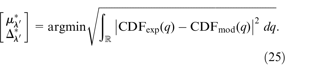
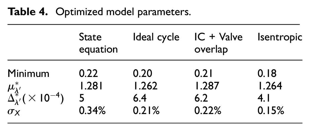
The functions used for developing the control-oriented model described by equations (21) and (22) have three parameters that need calibration: ${\mu }_{\lambda \prime }$ , ${\mathrm{\Delta }}_{\lambda \prime }$ , and ${\sigma }_X$ . The parameter ${\sigma }_X$ can be calculated from the distribution of the residuals from the regression $f_X(·)$ . In order to find the sigmoid parameters ${\mu }_{{\lambda }^{\prime }}$ and ${\mathrm{\Delta }}_{\lambda \prime }$ , consider solving the following optimization problem:

$$\left[\begin{array}{c}{\mu }_{\lambda \prime }^{*}\hfill \\ \multicolumn{1}{c}{{\mathrm{\Delta }}_{\lambda \prime }^{*}}\end{array}\right]=\mathrm{argmin}\sqrt{{\int }_{\mathbb{R}}{|\mathrm{CD}{\mathrm{F}}_{\exp }(q)-\mathrm{CD}{\mathrm{F}}_{\mathrm{mod}}(q)|}^2\mathrm{dq}}.$$

(25)

The cost function in equation (25) is an $L^2$ norm that measures the difference between the experimental cumulative distribution function (CDF) of $Q_{\mathrm{gross}}$ and the simulated CDF obtained using the proposed models. Due to the nonlinear nature of the system, steady-state CDFs for different combinations of ${\mu }_{\lambda \prime }$ , and ${\mathrm{\Delta }}_{\lambda \prime }$ were estimated by simulating the model during 10,000 cycles. The minimizer was found after an exhaustive search over a narrow domain of possible ${\mu }_{\lambda \prime }$ , and ${\mathrm{\Delta }}_{\lambda \prime }$ values. Table 4 shows the result of the optimization for the various methods. Note that the results from the Fitzgerald estimation method have been omitted due to its similarity with the isentropic method. The isentropic approach generates the lowest value for the cost function, which implies that it approximates the experimental CDF with the highest accuracy. The state equation and valve overlap methods present the highest values for the optimal ${\mu }_{\lambda \prime }^{*}$ since they generate the highest estimates for the residual fraction. The optimal value for the parameter ${\mathrm{\Delta }}_{\lambda \prime }^{*}$ has a similar magnitude for all methods. However, the isentropic approach presents the smallest ${\mathrm{\Delta }}_{\lambda \prime }^{*}$ , which translates to the fastest drop in efficiency at the ignition limit described by the sigmoid function. Recall that the parameter ${\sigma }_X$ measures the level of dispersion of the simulated $X_{\mathrm{res}}$ . Therefore, in order to generate the best approximation for the experimental CDF, the state equation method requires the highest dispersion for $X_{\mathrm{res}}$ while the isentropic method requires the lowest dispersion.

Table 4.

Optimized model parameters.

	Stateequation	Ideal cycle	IC + Valveoverlap	Isentropic
Minimum	0.22	0.20	0.21	0.18
${\mu }_{\lambda \prime }^{*}$	1.281	1.262	1.287	1.264
${\mathrm{\Delta }}_{\lambda \prime }^{*}(\times {10}^{-4})$	5	6.4	6.2	4.1
${\sigma }_X$	0.34%	0.21%	0.22%	0.15%

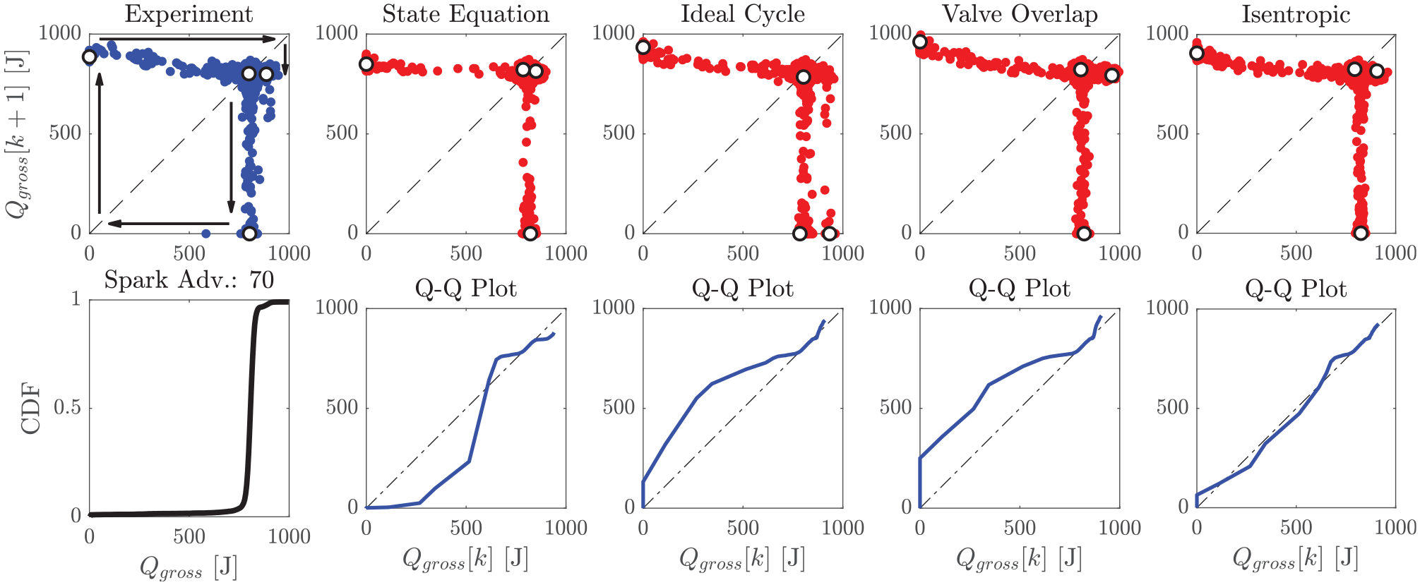
The optimal model parameters were used in simulations to compare not only the agreement with the experimental CDF but also to evaluate the ability to capture deterministic prior-cycle correlations. Combustion dynamics can be captured by return maps, which show the effect of cycle $k$ on the next combustion cycle $k+1$ . The quantile-quantile (Q-Q) plot was used as a graphical comparison between the simulated distribution and the experimental CDF of $Q_{\mathrm{gross}}$ . Figure 9 summarizes the results for different estimation methods using return maps and Q-Q plots for the experimental condition at 70 [deg bTDC] spark advance. As an example, the left column of Figure 9 shows the return map and the CDF of the experimental data using the isentropic method. As previously discussed, the cycle-to-cycle values of the experimental $Q_{\mathrm{gross}}$ are expected to be similar when using either the ideal cycle, valve overlap, isentropic, or Fitzgerald methods.

Figure 9.

Top row: Comparison between the dynamic response of the experimental $Q_{\mathrm{gross}}$ (top-left) and the simulated values using different residual fraction estimation methods. Bottom row: Experimental cumulative distribution function of $Q_{\mathrm{gross}}$ (bottom-left) and quantile-quantile plots comparing simulated ( $y$ -axis) and experimental ( $x$ -axis) CDFs.

The main prior-cycle correlation effect occurs when a misfire is followed by a high-energy cycle. This is pictured by the arrows on the top-left plot which follow the sequence of white dots: Nominal → Misfire → High-energy → Nominal. The CDF of $Q_{\mathrm{gross}}$ shows a rapid increase around the nominal value of 806 [J], which indicates that most of the cycles are distributed around such a value. The top row of Figure 9 shows (in red) the return maps obtained from simulations using the same random sequences for $\{w[k]\}$ and $\{v[k]\}$ but different modeling strategies. A similar set of white dots are highlighted which correspond to cycles preceding and following a misfire. The bottom row of Figure 9 shows the Q-Q plots with the simulated distribution on the $y$ -axis and the corresponding experimental distribution on the $x$ -axis. When the combustion CCV is modeled using the state equation method, the return map shows an inability to capture prior-cycle correlation. In this case, misfires are not followed by high-energy cycles but rather the system stabilizes immediately. These discrepancies are also observed in the Q-Q plot for low-energy and high-energy values. Similarly, modeling the system based on the ideal cycle analysis generates prior-cycle correlations different from the ones experimentally observed. In this case, some simulated sequences of cycles have the deterministic pattern: Nominal → Misfire → High-energy → Misfire. On the other hand, the ideal cycle with valve overlap and isentropic methods can mimic the prior-cycle correlation from experimental data. In addition, the Q-Q plot shows a good agreement between the experimental and the simulated distributions. Note that, even though the ideal cycle and ideal cycle with valve overlap approaches have similar assumptions, the simulated result produces different combustion dynamics. This is a result of the regressed function $f_X(·)$ . Recall that in the ideal cycle method the values for $X_{\mathrm{res}}$ remained virtually constant for nominal and high-energy cycles. For the valve overlap and isentropic methods, however, $X_{\mathrm{res}}$ during nominal cycles is greater than $X_{\mathrm{res}}$ during high-energy cycles. This difference appears to be key for capturing the correct dynamic behavior.

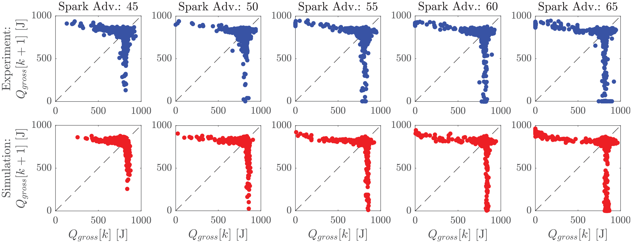
The experimental validation for the different methods, however, was performed at a significantly advanced spark of 70 [deg bTDC]. At this condition, the CCV is dominated by sporadic misfires and the next-cycle dynamics previously discussed are easily observed. If the same levels of EGR are maintained, retarding the spark generates a different CCV behavior favoring the occurrence of partial burns. ²⁵ The top row of Figure 10 shows the experimental return maps of $Q_{\mathrm{gross}}$ for conditions with spark advance between 45 and 65 [deg bTDC]. As spark retards, the number of misfires recorded in 5000 cycles steadily decreases until they are nonexistent at 45 [deg bTDC] spark. The control-oriented model was used to simulate all operating conditions using the isentropic assumption for the residual gas fraction functional dependency $X_{\mathrm{res}}[k]=f_X(Q_{\mathrm{gross}}[k])$ . The sigmoid function parameters for all conditions were calibrated using the proposed optimization problem in equation (25). The bottom row of Figure 10 shows the return maps obtained after simulations, showing a close agreement with experiments. Such simulations demonstrate the versatility of the model and the calibration procedure for simulating conditions at the ignition limit at either partial burn or misfire-dominated conditions.

Figure 10.

Comparison between experimental (top row) and simulated (bottom row) return maps for $Q_{\mathrm{gross}}$ using the isentropic assumption for residual gas fraction estimation at different values of spark advance.

All in all, control-oriented models using the functional dependency $X_{\mathrm{res}}[k]=f_X(Q_{\mathrm{gross}}[k])$ can be useful for capturing the probability distribution and the combustion dynamics of the experimental $Q_{\mathrm{gross}}$ . The function $f_X(·)$ , however, depends on the residual fraction estimation method utilized. The results show that only the ideal cycle with valve overlap and the isentropic methods can generate simulated data that mimic experimental observations of dynamics observed after misfire events. The Fitzgerald method was not considered for further analysis since it produces the same level of accuracy and dynamic behavior as the isentropic method. In the case that the valve overlap is significant, however, the ideal cycle with valve overlap method should be preferred. Otherwise, the isentropic method presents a clear modeling advantage given its computational simplicity.

Conclusion and outlook

The combustion model originally presented by Daw et al. ⁹ describes the cycle-to-cycle combustion dynamics of spark-ignition engines. Here, the residual gas composition from one cycle to the next acts as the coupling mechanism, which is especially important during partial burns and misfires where most of the residual composition is unburned gas. Several articles in the literature have proposed different methods for residual gas fraction estimation. Nonetheless, not all methods yield accurate functional dependencies for offline simulation of combustion CVV.

The first approach considered was the state equation, which applies the in-cylinder ideal gas law at EVC but uses the measured exhaust manifold temperature. This method was unable to capture significant cycle-to-cycle patterns in the residual gas estimation. The second approach considered an ideal thermodynamic cycle analysis. This procedure solves a constant-volume combustion cycle from start to finish assuming that the residual gas in the current cycle equals the residual gas transferred to the next. This approach can capture the functional relationship between the residual fraction and the gross heat release, but fails at providing an accurate model for offline simulations.

The third approach is based on the ideal cycle analysis but includes the effect of valve overlap. Here, high-speed intake and exhaust manifold pressure sensors were used to quantify the amount of backflow from the exhaust manifold into the cylinder during valve overlap. The extra information gathered by the sensors during this period produced an accurate estimation and modeling of the residual gas. The isentropic method was originally proposed by Yun and Mirsky ¹⁸ and requires only the in-cylinder pressure and volume information at EVO and EVC. Although the qualitative properties of the combustion dynamics are similar to the ideal cycle with valve overlap method, different trends could be observed that highlight the fundamental differences between these approaches. Finally, the method proposed by Fitzgerald et al. ¹⁹ was discussed. Such a method applies the unsteady first law of thermodynamics to the exhaust process in order to include convective heat transfer effects. However, it was found that, for this particular application, the Fitzgerald method was equivalent to the isentropic estimation method.

All such methods were compared based on (1) the gross heat release estimates and (2) the functional dependencies $X_{\mathrm{res}}[k]=f_X(Q_{\mathrm{gross}}[k])$ which allow offline simulation. The results showed that the state equation method is the only outlier, with a significant difference compared with the other methods when gross heat release is evaluated. Therefore, the ideal cycle, ideal cycle with valve overlap, isentropic, and Fitzgerald methods generate similar estimates, even though the residual gas fraction values might differ. It was shown that a cycle-to-cycle control-oriented combustion model depends on the residual gas estimation method. Moreover, it was observed that the residual fraction can be described by a function of the gross heat release. Simulations based on the different residual gas estimation methods showed that the ideal cycle with valve overlap, isentropic, and Fitzgerald methods were the only ones able to capture the effects of misfires on future combustion events observed in experiments. However, computational limitations on commercial engine control units and time constraints imposed by engine speed favor the implementation of the isentropic method when online parameter estimation is required.

Additionally, the modeling and calibration approach presented in this study was utilized to simulate the gross heat release at different levels of spark advance. The results showed that the isentropic method for estimating residual gas fraction can be used to accurately simulate CCV characteristics observed during misfire-dominated conditions (advanced spark) and partial burn-dominated conditions (retarded spark) with comparable levels of accuracy.