Sage Journals: Discover world-class research

Abstract

In this work, a hybrid breakup model tailored for direct-injection spark-ignition engine sprays is developed and implemented in the OpenFOAM CFD code. The model uses the Lagrangian–Eulerian approach whereby parcels of liquid fuel are injected into the computational domain. Atomization and breakup of the liquid parcels are described by two sub-models based on the breakup mechanisms reported in the literature. Evaluation of the model has been carried out by comparing large-eddy simulation results with experimental measurements under multiple direct-injection spark-ignition engine-like conditions. Spray characteristics including liquid and vapor penetration curves, droplet velocities, and Sauter mean diameter distributions are examined in detail. The model has been found to perform well for the spray conditions considered in this work. Results also show that after the end of injection, most of the residual droplets that are still in the breakup process are driven by the bag and bag–stamen breakup mechanisms. Finally, an effort to unify the breakup length parameter is made, and the given value is tested under various ambient density and temperature conditions. The predicted trends follow the measured data closely for the penetration rates, even though the model is not specifically tuned for individual cases.

Keywords

Large-eddy simulation fuel sprays atomization breakup spray modeling direct-injection spark-ignition gasoline engines

Introduction

Performance and operation of direct-injection spark-ignition (DISI) engines rely heavily on the fuel injection and subsequent fuel–air mixing quality, especially for the spray-guided DISI combustion systems.¹ The fuel injector is the most critical part of DISI fuel systems, and its design needs to meet more stringent requirements than that of the port-fuel injector. Modern DISI injectors have a multi-hole design similar to that used in diesel engines. Unlike the hollow-cone swirl-type injectors, the spray characteristics of this configuration have been proven to have less dependence on ambient conditions. It also has the flexibility to direct spray plumes at desired locations to help meet the combustion system requirements.²

Atomization, or primary breakup, refers to the disintegration of liquid jet or liquid core into ligaments and droplets at the nozzle exit. Atomization provides initial conditions for droplet breakup and the subsequent fuel–air mixing process. In general, higher injection pressure results in faster atomization. However, it has been found that higher injection pressure does not necessarily lead to smaller droplet sizes in diesel sprays.³ This suggests that droplet breakup and collision are more important determining factors of the mixing process. A recent study by Baumgarten⁴ found that the disintegration of high-pressure diesel sprays begins inside the nozzle-hole, hence the liquid core does not exist. For modern DISI injectors, the relatively small length-to-diameter (L/D) ratios and volatile fuel components promote complex turbulent flows and phase-change phenomena such as cavitation and flash boiling, which suppress the formation of the liquid core. Therefore, liquid fuel near the injector exit may contain only droplets and ligaments. The highly turbulent two-phase internal flows also make the modeling of atomization a particularly difficult challenge.

One way to overcome the challenge of atomization modeling is to perform direct numerical simulations (DNS) to resolve the atomization completely. These can be achieved by Eulerian representation of the turbulent two-phase flow with an interface tracking approach such as the volume of fluid (VOF) or level set (LS) methods. However, the computational requirements for DNS are extremely challenging so that its practical applications are still under development.⁵ Therefore, phenomenological approaches using Lagrangian representations of liquid fuel still remain the most popular methods for atomization modeling in engine applications.^6–8 A reasonable approximation is to inject fuel parcels with a characteristic size equal to the nozzle orifice diameter (i.e. the blob method).⁹ Other reported work also utilizes a prescribed probability density function (PDF) for the initial parcel size distribution to mimic the atomization process.⁶ In this approach, however, the PDF must be guessed and tuned to match spray characteristics further downstream of the injector exit. Modeling efforts focused on the atomization induced by internal turbulence and cavitation were also reported and encouraging results were obtained.^7,10,11 One issue of these methods is that one-dimensional (1D) modeling of the internal flow is usually needed, which requires detailed information about the nozzle geometry. Moreover, only one atomization mode (e.g. cavitation, turbulence, or flash boiling) is normally considered.

Compared to the diesel counterpart, DISI injectors operate at much lower system pressure, resulting in several times lower liquid velocity at the nozzle exit. Gasoline fuel also has a lower density and viscosity than diesel fuel. As a result, the governing non-dimensional numbers in droplet breakup, such as the Weber number and the Ohnesorge number, are generally smaller in gasoline sprays. The Weber number and Ohnesorge number are defined as $We = ρ_{g} U_{rel}^{2} d_{d} / σ$ and $Oh = μ_{l} / \sqrt{ρ_{l} d_{d} σ}$ , where $ρ_{g}, d_{d}, μ_{l}, and σ$ are the gas-phase density, droplet diameter, liquid-phase viscosity, and surface tension, respectively. This difference is demonstrated in Figure 1, where a map of droplet breakup regimes as functions of We and Oh numbers is plotted.¹² In the map, the We–Oh diagrams of typical gasoline and diesel sprays are enclosed with dashed and dotted lines, respectively. As Figure 1 shows, there is only a small overlap between diesel and gasoline sprays, implying that the governing breakup mechanisms are vastly different. Most diesel droplets break owing to either catastrophic or sheet-thinning mechanisms. However, gasoline sprays shift to the lower left region in the map and a unique breakup mechanism, namely, the bag breakup, becomes more pronounced.

Figure 1.

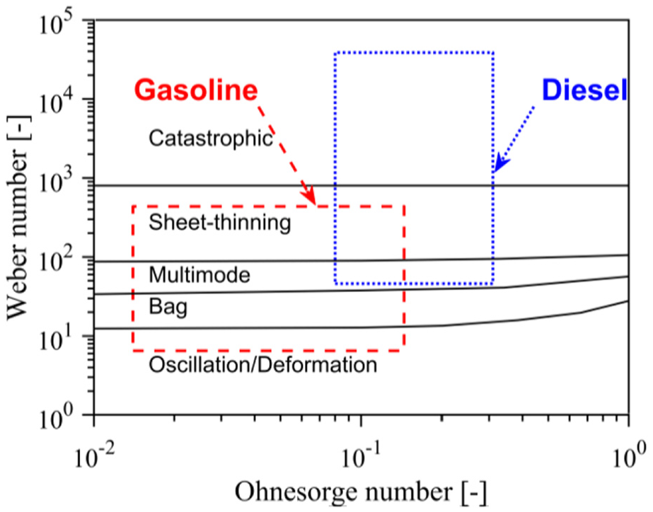
Map of droplet breakup regimes as functions of Weber and Ohnesorge numbers.¹² The breakup regimes of typical gasoline and diesel sprays are enclosed by dashed and dotted lines, respectively.

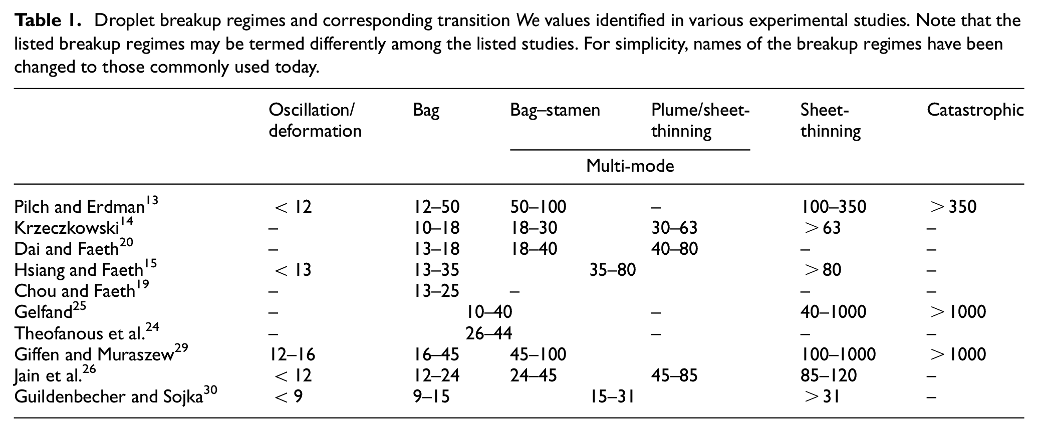
The droplet breakup regimes depicted in Figure 1 have been extensively studied by various researchers. Selected references on this topic are those of Pilch and Erdman,¹³ Krzeczkowski,¹⁴ Faeth et al.,^15–20 Liu and Reitz,²¹ Reitz and Lee,²² Opfer et al.,²³ Theofanous et al.,²⁴ Gelfand,²⁵ Jain et al.,²⁶ and Girin.²⁷ Detailed descriptions of each breakup regime can be found in the above references or a recent review by Guildenbecher et al.²⁸ It has been generally accepted that the transitions among different breakup regimes are continuous functions of We and Oh.²⁸ Some experimental studies also show that the transitions are nearly independent of Oh for Oh less than 0.1.¹⁷ In Table 1, the droplet breakup regimes identified in various studies are reported along with the transition We. Note that the inconsistencies in reported We values among listed studies are primarily due to the experimental uncertainties (non-sphericity of droplets and uncertainties associated with velocity measurements) and the fact that the transitions are continuous processes.

Table 1.

Droplet breakup regimes and corresponding transition We values identified in various experimental studies. Note that the listed breakup regimes may be termed differently among the listed studies. For simplicity, names of the breakup regimes have been changed to those commonly used today.

	Oscillation/deformation	Bag	Bag–stamen	Plume/sheet-thinning	Sheet-thinning	Catastrophic
	Oscillation/deformation	Bag	Multi-mode		Sheet-thinning	Catastrophic
Pilch and Erdman¹³	<12	12–50	50–100	–	100–350	>350
Krzeczkowski¹⁴	–	10–18	18–30	30–63	>63	–
Dai and Faeth²⁰	–	13–18	18–40	40–80	–	–
Hsiang and Faeth¹⁵	<13	13–35	35–80		>80	–
Chou and Faeth¹⁹	–	13–25	–		–	–
Gelfand²⁵	–	10–40		–	40–1000	>1000
Theofanous et al.²⁴	–	26–44		–	–	–
Giffen and Muraszew²⁹	12–16	16–45	45–100		100–1000	>1000
Jain et al.²⁶	<12	12–24	24–45	45–85	85–120	–
Guildenbecher and Sojka³⁰	<9	9–15	15–31		>31	–

Most of the earlier research on large-eddy simulation (LES) of DISI sprays was conducted by combining spray models with a LES turbulence closure. Some of these studies have utilized the Taylor analogy breakup (TAB) models.^31–33 While this approach can give satisfactory results under certain DISI operating conditions, it has a few shortcomings such as the somewhat arbitrary breakup criteria and the assumption of instantaneous breakup.^12,28 Recently, Van Dam and Rutland³⁴ explored the possibility of applying a diesel-type breakup model to DISI gasoline sprays. The Kelvin–Helmholtz/Rayleigh–Taylor (KH-RT) breakup model was validated against DISI spray experiments in a constant volume chamber over a wide range of ambient conditions. A functional relationship between the KH-RT model parameters and the liquid-gas density ratio was found after carefully calibrating the KH-RT model. Although this functional relationship was found to give good vapor contours compared to Schlieren images, discrepancies were noted for both liquid and vapor penetration rates. The addressing of bag breakup in DISI engines is even more scarce in the literature, even though various numerical models have been reported.^23,35–37 Chryssakis and Assanis¹⁰ proposed a unified approach for both diesel and gasoline engine applications. In their model, the droplet breakup has been divided into four regimes, namely, the bag, multi-mode, shear, and catastrophic regimes. Sub-models or correlations have been proposed in this unified approach to describe each breakup regime. The model has been found to perform well under both diesel and gasoline engine conditions. However, the validation was carried out at non-evaporating conditions. The application of this model under high-temperature high-pressure engine-like conditions has yet to be demonstrated.

This work is aimed to develop a physically representative breakup model for DISI gasoline sprays. The model, termed as the “integrated atomization/breakup (IAB) model,” builds on previous modeling efforts by incorporating a bag breakup model developed by the authors and addressing the breakup issues of droplets at relatively low We conditions. The model does not treat atomization and droplet breakup as separate processes. Instead, liquid ligaments and droplets are assumed to form immediately at the nozzle exit, and two sub-models are employed to describe the subsequent atomization/breakup processes. A revised breakup length concept is also employed to account for different penetration rates near and far from the nozzle. However, this concept should not be confused with the liquid core length, which normally implies that liquid jet or ligaments within this length experience atomization only. This conceptual difference was also noted by Beale and Reitz.³⁸ In their work, certain parcels within the breakup length are also assumed to experience droplet breakup. The IAB model has been incorporated into the LES framework developed at the Engine Research Center, University of Wisconsin–Madison, and implemented in the three-dimensional (3D) CFD code OpenFOAM-2.3.x.³⁹ Validation of the model has been performed by comparing LES predictions with experimental data. In the remaining of this article, detailed discussions of the model and results will be provided as follows. Section “IAB model” presents the formulations of the IAB model. Sections “Spray experiments for comparison” and “Simulation setup” discuss the spray experiments for validations and the numerical setup. In section “Results and discussion,” we discuss both the numerical and experimental results. Finally, concluding remarks and future directions are made in section “Summary and conclusion.”

IAB model

The IAB model relies on the well-known KH-RT hybrid model to describe the atomization of liquid fuel and breakup process of liquid ligaments and droplets in the plume-sheet thinning, sheet-thinning, and catastrophic breakup regimes depicted in Figure 1. Note that even though this model was developed based on linear stability theories (hence not physically suitable for the multi-mode breakup), it has been found to perform reasonably well for diesel sprays,^38,40 which also experience multi-mode breakup. Besides, multi-mode breakup resembles a combination of bag and sheet-thinning breakup and hence constructing a numerical model for this specific regime is still impractical. Therefore, the multi-mode breakup regime is not treated separately in the IAB model. The IAB model also utilizes a phenomenological bag-breakup model to describe the breakup process in the bag and bag–stamen regimes.⁴¹ The KH-RT sub-model will be briefly reviewed first, followed by the descriptions of the bag sub-model and the IAB model implementation.

The KH-RT sub-model

In the catastrophic breakup regime, the dynamic pressure on the droplet surface becomes very large, causing unstable waves to grow on the droplet leading surface. Liu et al.⁴² suggested that those unstable waves may be described by either Rayleigh–Taylor (RT) or Kelvin–Helmholtz (KH) instabilities. RT unstable waves form when a density discontinuity is accelerated toward the lighter end, which eventually penetrate the denser droplet and create several small droplets. KH instabilities occur at the droplet periphery where the relative velocity is the largest. Wavelengths of KH instabilities are much shorter compared to those of RT, leading to micro-size droplets being continuously stripped from KH waves.

The KH-RT hybrid model refers to the one developed by Su et al.⁴³ based on the work of Reitz and Diwakar⁴⁴ and Reitz.⁴⁵ The model was later improved by Ricart et al.⁴⁰ by introducing the RT breakup length to account for different penetration rates within and beyond a certain distance from the nozzle exit. The model was divided into two sub-models, namely, the KH breakup model and the RT breakup model. The former was derived based on a linear stability analysis of a cylindrical liquid surface subjecting to an infinitesimal perturbation.⁴⁵ The dispersion relation between the growth rate of this perturbation and its wavenumber was determined. Curve-fits of the numerical solutions were further generated for the maximum wave growth rate, $Ω_{KH}$ , and the corresponding wavelength, $Λ_{KH}$

\begin{array}{l} Ω_{K H} = \frac{0.34 + 0.134 W e^{1.5}}{(1 + 1.414 O h) (1 + 1.4 T a^{0.6})} \sqrt{\frac{8 σ}{ρ_{l} d_{d}^{3}}} \\ Λ_{K H} = \frac{4.51 d_{d} (1 + 0.535 \sqrt{O h}) (1 + 0.4 T a^{0.7})}{{(1 + 0.272 W e^{1.67})}^{0.6}} \end{array}

(1)

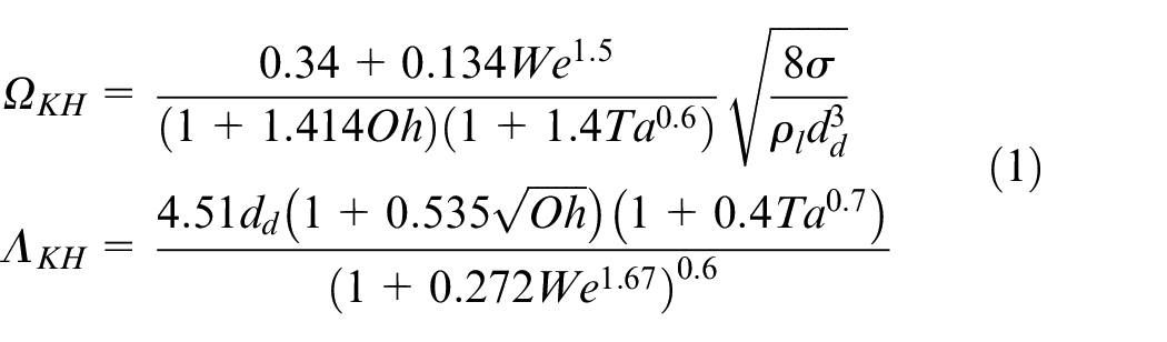
where Ta is the Taylor number defined as $Ta = Oh \sqrt{We}$ . Note that equation (1) was originally given in terms of droplet radius.⁴⁵ In this work, it is given in terms of droplet diameter to be consistent with the remaining of the IAB model. Child droplets are formed with a diameter $d_{c}$ , such that $d_{c} = 2 B_{0} Λ_{KH}$ with the constant $B_{0} = 0.61$ . The rate of change of parent droplet diameter is then inversely proportional to the KH time constant $τ_{KH} = 1.836 B_{1} d_{d} / Λ_{KH} Ω_{KH}$ , where $B_{1}$ is an adjustable model parameter with a typical range between 10 and 100.

RT unstable waves are due to droplet acceleration or deceleration. The fastest-growing frequency, $Ω_{RT}$ , and the corresponding wavelength, $Λ_{RT}$ , are given by

\begin{matrix} Ω_{RT} = \sqrt{\frac{2}{3 \sqrt{3 σ}} \frac{{[- g (ρ_{l} - ρ_{g})]}^{3 / 2}}{ρ_{l} + ρ_{g}}} \\ Λ_{RT} = 2 π C_{RT} \sqrt{\frac{- 3 σ}{g (ρ_{l} - ρ_{g})}} \end{matrix}

(2)

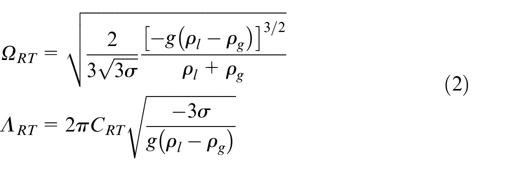
where g is the acceleration in the direction of travel and $C_{RT}$ is a model parameter typically set to 0.1. The growth time of RT unstable wave is tracked if the wavelength $Λ_{RT}$ is smaller than the droplet diameter. The droplet is assumed to break if the growth time exceeds the RT breakup time, $τ_{RT} = C_{τ} / Ω_{RT}$ , where $C_{τ}$ is a model parameter typically set to 1.0. The diameter of child droplets is assumed to be $Λ_{RT}$ .

The KH-RT hybrid model builds on the idea that only the KH breakup is activated if the distance between liquid parcels and the nozzle exit is within a pre-calculated breakup length, $L_{B}$ . Beyond that length, both KH and RT unstable waves compete to break the droplet. In the revised model by Ricart et al.⁴⁰ and Tsang,⁴⁶ the breakup length is computed as

L_{B} = 9.12 C_{b} d_{noz} \sqrt{\frac{ρ_{l}}{ρ_{g}}}

(3)

where $d_{noz}$ is the nozzle diameter and $C_{b}$ is a model parameter. Although the breakup length is conceptually considered as a global parameter, its value may be different among fuel parcels depending on the local fuel–air density ratios. In this study, the breakup length is calculated according to the following formula

L_{B} = 9.12 \frac{\sqrt{C_{a}} d_{noz}}{α \sin (θ)} \sqrt{\frac{ρ_{l}}{ρ_{g}}}

(4)

where $C_{a}$ is the area contraction coefficient, $α$ is a model parameter, and $θ$ is the plume direction (i.e. the spray axis angle). Note that there is no typical range for $α$ , as setting it to a large positive number will effectively disable $L_{B}$ , leading to faster breakup and lower penetration. Contrarily, RT breakup will be disabled if $α$ is zero. In our experience, equation (4) works well for $θ$ in the range between 25° and 55°. Although it has not been tested for $θ$ beyond this range as there are limited experimental data for validation, it is expected to work reasonably well. Equation (4) is proposed based on the mixing-limited vaporization model of Siebers,⁴⁷ where $L_{B}$ projected to the injector centerline is proportional to the characteristic liquid length defined in Siebers.⁴⁷ Although the model was developed for diesel sprays, it can be applied to multi-plume DISI sprays with some success.⁴⁸ In equation (4), the product of the square root of the area contraction coefficient and the nozzle diameter equals the effective nozzle diameter. The impact of plume interactions is considered by taking the sine of the plume direction.

The bag sub-model

The physical mechanisms involved in bag breakup are very complicated. Experimental studies can hardly measure the local droplet and gas flow fields that lead to the formation and disintegration of the bag structure. However, it is generally observed that a thin hollow membrane-like bag forms at the front stagnation point of the deformed droplet and continues to be blown downstream. The bag bursts first, leaving a few small fragments and a liquid torus ring. The latter will eventually break into a few child droplets.¹⁹ A phenomenological model for the bag and bag–stamen breakup is developed based on the experimental observations of Chou and Faeth.¹⁹ In this model, the breakup process is divided into three stages as illustrated in Figure 2: (a) deformation and bag growth stage, during which the droplet deforms from its initial spherical shape into a liquid disk and forms a continuously growing thick membrane-like bag; (b) bag rupture stage, where the bag bursts into a liquid torus ring and many micro-size droplets; and finally, (c) torus breakup stage, where the torus ring breaks into a few child droplets. Two characteristic sizes are expected, one corresponding to the bag rupture and the other to the torus breakup. As a consequence, a bi-modal droplet size distribution may be observed.^28,36

Figure 2.

Schematic of the bag breakup process:²³ (a) bag growth, (b) bag rupture, and (c) torus breakup. A bi-modal droplet size distribution may be observed after the bag rupture and torus breakup.

During the first stage of the breakup process, the rate of droplet deformation or bag growth can be quantified by the ratio of the cross-stream diameter $d_{b}$ to the initial droplet diameter $d_{d 0}$ . A semi-theoretical model has been developed by the authors to describe the deformation and bag growth process.⁴¹ Droplet dynamics were analyzed by subjecting a liquid droplet to an inviscid, incompressible ambient flow. The solution of the resulting equations gives the following expression to describe the droplet deformation and bag growing process, which relates the diameter ratio with a non-dimensional time $t^{*}$ and the initial droplet Weber number, $W e_{0}$

\begin{matrix} \frac{d_{b}}{d_{d 0}} = f (t^{*}, W e_{0}) \\ = \exp [C_{bag, g} t^{*^{2}} \sqrt{(1 - \frac{6}{W e_{0}})}], 0 < t^{*} < τ_{bag} \end{matrix}

(5)

where $t^{*}$ is the ratio of elapsed time t to a non-dimensional characteristic time proposed by Nicholls and Ranger,⁴⁹ $T^{*} = d_{d 0} (ρ_{l} / ρ_{g})^{0.5} / U_{rel}$ . Equation (5) is valid only when the non-dimensional time is smaller than $τ_{bag}$ , which is defined as the non-dimensional time when the bag ruptures. A model parameter $C_{bag, g}$ is also introduced in equation (5), whose value is determined by curve fitting of the experimental data from Kulkarni³⁶

C_{bag, g} = [0.2983 - \frac{0.2691}{1 + {(\frac{W e_{0}}{14.013})}^{13.629}}]

(6)

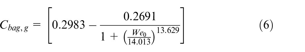
Chou and Faeth¹⁹ observed that the bag rupture starts at approximately $t^{*} = 3$ , while Opfer et al.²³ identified the rupture to happen at about $t^{*} = 2$ . In this study, the onset time of bag rupture $τ_{bag}$ is determined using a correlation based on the experimental data from Opfer et al.²³

τ_{bag} = \frac{C_{bag, r}}{1.0 - \frac{1.018}{{We}_{0}^{0.1818}}}

(7)

where $C_{bag, r}$ is a model parameter with a nominal value of 0.8. The coefficient of determination (i.e. R²) of this correlation is 0.999, and the corresponding root mean square error (RMSE) is 0.037. Predicted onset times using equation (7) are plotted in Figure 3 as a function of We, for Oh less than 0.1. The plotted results also include experimental data from Opfer et al.,²³ Krzeczkowski,¹⁴ Dai and Faeth,²⁰ and VOF predictions from Jian et al.,²⁶ Liang et al.,⁵⁰ and Khosla et al.⁵¹ The We range spans from the bag to sheet-thinning breakup regimes. As Figure 3 shows, the qualitative trend of the onset time is well captured by the correlation. The RMSE of equation (7) increases to 0.24 if the VOF results are also taken into consideration. The experimental data from Krzeczkowski¹⁴ and Dai and Faeth²⁰ seem to be outliers, which may be attributed to the vague definition of $t^{*} = 0$ among different studies. In this work and the VOF studies reported in Figure 3, $t^{*} = 0$ is defined as the time when the droplet enters the disruptive gas field. In the shock tube experiments by Dai and Faeth,²⁰ $t^{*} = 0$ may be defined as the time when the diaphragm ruptures. The cross-flow measurement results from Krzeczkowski¹⁴ lie even further away from plotted data. The reason of this rather large deviation is unknown to the authors.

Figure 3.

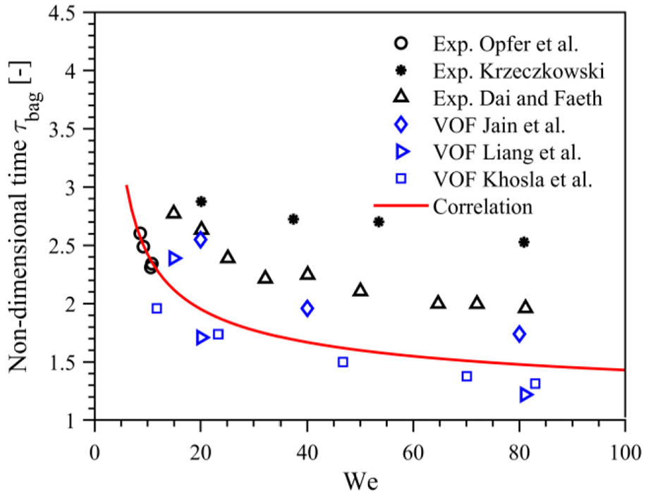
Measured and predicted non-dimensional onsite time of bag rupture as a function of We number. Continuous results obtained from the present correlation are plotted as a solid line. Data from the literature are plotted as symbols.

It is important to know the relative volume fraction of the bag and the remaining liquid torus in order to estimate the child droplet size. Chou and Faeth¹⁹ showed that the liquid bag may contain about half of the initial droplet volume. Assuming the liquid bag attached to the torus has a hemispherical shape, the bag thickness $h_{bag}$ is determined from mass conservation of the droplet

h_{bag} = \frac{ϕ_{bag} d_{d 0}}{3.0} \frac{1.0}{{[f (t^{*}, W e_{0}) |_{t^{*} = τ_{bag}}]}^{2}}

(8)

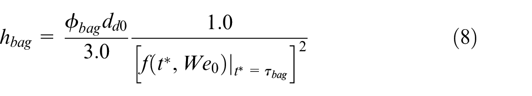
where $ϕ_{bag}$ is the volume fraction of the liquid bag when it ruptures. Child droplets formed after the bag rupture are assumed to have a size proportional to the bag thickness, $d_{c} = C_{bag, rc} h_{bag}$ , where $C_{bag, rc}$ is an adjustable constant with a nominal value of one.

After the bag rupture, the remaining liquid torus ring is assumed to continuously expand outwardly in the cross-stream direction with a constant rate, $\partial f (t^{*}, W e_{0}) / \partial t^{*} |_{t^{*} = τ_{bag}}$ . The torus eventually breaks into a few child droplets due to RT-related instabilities.^18,52 Thus, the breakup in this stage is tracked by the RT unstable waves. The frequency of the fastest-growing RT wave and its wavelength are calculated using equation (2). RT wave is assumed to grow on the liquid torus surface if its wavelength is smaller than the liquid torus diameter, $d_{b} = f (t^{*}, W e_{0}) d_{d 0}$ . Once the wave begins to grow, the growth time is tracked and compared to the RT breakup time, $τ_{RT}$ . The torus is assumed to break if the elapsed time is larger than $τ_{RT}$ . The diameter of child droplets is equal to the torus tube diameter, $d_{r}$ , which can be computed from mass conservation.

Model implementation

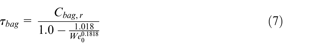
A flowchart of the IAB model is provided in Figure 4. Note that the choice of sub-model depends on the droplet We number. If $We < W e_{crit}$ , no breakup is assumed to happen since the droplet is in the oscillation/deformation breakup regime. This oscillation breakup does not happen in every instance, and even when it occurs, the overall breakup time is much longer compared to the other mechanisms listed in Table 1. Therefore, as a common approach,²⁸ this work ignores the oscillation/deformation breakup and takes the bag breakup as the first breakup regime. If $W e_{crit} < We < W e_{bag}$ , the phenomenological bag breakup sub-model is used. Finally, if $We > W e_{bag}$ , the revised KH-RT model is used. The value of $W e_{crit}$ is generally set to 12, although lower values (≈7) were found in the literature.^24,27 In this work, its value is set to 6 since in equation (5), droplets with We larger than 6 are predicted to form a slowly growing bag structure. However, in our experience, changing the value of $W e_{crit}$ from 6 to 12 seems to have little impact on the spray characteristics. The transitional Weber number $W e_{bag}$ is negatively correlated with the predicted liquid penetration, based on the findings from a previous uncertainty quantification (UQ) study.⁵³ The reported values of $W e_{bag}$ in Table 1 range from 18 to 100. In this work, it is set to 56, a value roughly equals the mean of the reported ones in Table 1.

Figure 4.

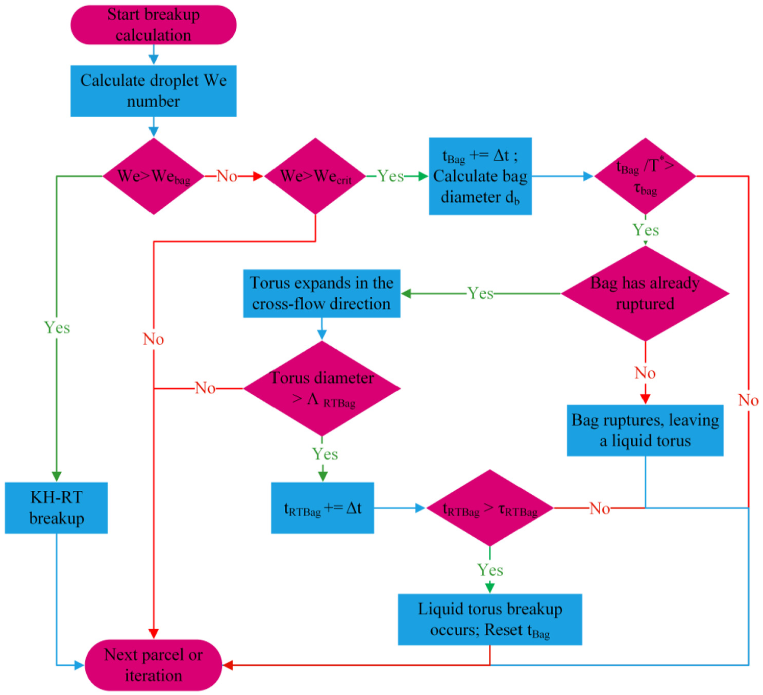
Flowchart of the IAB model. In this work, We_bag and We_crit are set to 56 and 6, respectively.

Spray experiments for comparison

The standard Spray G condition specified by the Engine Combustion Network (ECN) is used in this work to evaluate the IAB model. The ambient conditions correspond to a non-reacting early injection case in DISI engines.⁵⁴ The Spray G injector has eight symmetrically spaced holes, each with a nominal plume direction of 37°. Table 2 lists the injector specifications and operating conditions. More details can be found on the ECN website.⁵⁵ Another data set used for spray model validation, termed as the General Motors (GM) DISI sprays, are taken from the work of Parrish⁴⁸ and Parrish and Zink.⁵⁶ Measurements were conducted under late injection DISI engine-like conditions. Iso-octane was injected into a high-temperature pressure vessel by a multi-hole DISI injector. The injector has eight symmetrically spaced holes, each with an inlet orifice diameter of 0.140 mm. The measured plume direction of this injector is 25°. Continuous flow of nitrogen passing through the vessel is used to provide evacuation of fuel vapor and residual droplets. Test conditions and details of the injector are also listed in Table 2.

Table 2.

Operating conditions and injector specifications of ECN Spray G and GM DISI sprays.

Data type	ECN Spray G	GM DISI spray
Ambient gas density (kg/m³)	3.5	3, 6, 9
Ambient gas composition (–)	N₂, CO₂, H₂O	N₂
Ambient gas temperature (K)	573	400, 500, 600, 700, 800, 900
Ambient gas pressure (bar)	6.0	3.56–24.04
Ambient gas velocity (m/s)	≈0	≈0
Fuel temperature (K)	363	363
Injector orifice diameter (mm)	0.172	0.140
Injection pressure (MPa)	20.0	20.0
Injection duration (ms)	0.78	0.865
Injected fuel mass (mg)	10.0	10.0
Plume direction (°)	37	25

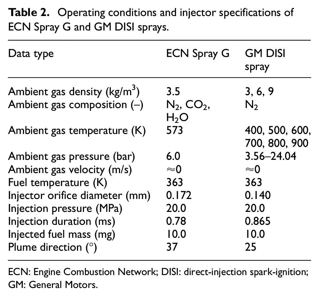
ECN: Engine Combustion Network; DISI: direct-injection spark-ignition; GM: General Motors.

Figure 5 summarizes the ambient conditions for both ECN Spray G and GM DISI spray experiments. Note that for GM DISI sprays, the spray characteristics were acquired with ambient temperatures ranging from 400 to 900 K at intervals of 100 K. At each temperature, three test conditions corresponding to ambient densities of 3.0, 6.0, and 9.0 kg/m³ were set by adjusting the ambient pressure. Four conditions, represented by circles on the figure, are selected to calibrate the IAB model and to obtain an optimal value of the IAB model parameter, $α .$

Figure 5.

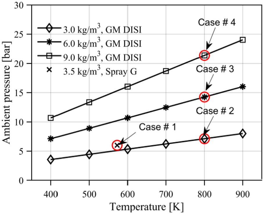
Experimental ambient conditions for ECN Spray G and GM DISI sprays. Symbols indicate conditions where experimental measurements were taken. Circles indicate four conditions where the model calibration was conducted.

Volume-illumination Mie-scatter and Schlieren images were taken at both institutions to understand the macroscopic spray characteristics such as the penetration rates and envelopes of both liquid and vapor phases.^48,57,58 Phase Doppler interferometry (PDI) measurements were also conducted for Spray G to measure the droplet velocity and Sauter mean diameter (SMD) distributions.⁵⁸ More information about the optical diagnostic devices and the difference between the experimental setups can be found in Parrish⁴⁸ and Manin et al.⁵⁷

Simulation setup

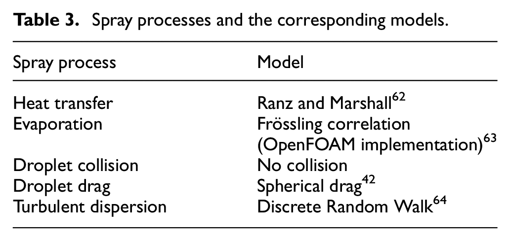
The OpenFOAM CFD code is used as the computational framework for running LES spray simulations.³⁹ A one-equation non-viscosity dynamic structure turbulence model⁵⁹ is used for turbulence modeling, wherein the transport equation of the sub-grid scale (SGS) turbulent kinetic energy, $k_{sgs}$ , was modified to include the LES spray term.⁶⁰ The energy dissipation term of the $k_{sgs}$ —transport equation also includes a parameter whose value is scaled with a characteristic length in order to reduce the mesh sensitivity of vapor-phase penetration.⁶¹ Other spray-related sub-models are listed in Table 3, along with the corresponding references. The initial parcel diameter is assumed to equal the effective nozzle diameter. Other spray boundary conditions such as the rate of injection (ROI) profiles, initial temperature, and plume direction and plume cone angles are taken from experimental measurements.^48,56,58

Table 3.

Spray processes and the corresponding models.

Spray process	Model
Heat transfer	Ranz and Marshall⁶²
Evaporation	Frössling correlation (OpenFOAM implementation)⁶³
Droplet collision	No collision
Droplet drag	Spherical drag⁴²
Turbulent dispersion	Discrete Random Walk⁶⁴

The vapor region in simulations is determined using a threshold of 0.1% local mixture fraction, as recommended by ECN⁶⁵ for standard Schlieren comparisons. Vapor penetration is then defined as the furthest axial distance between the injector tip and the vapor boundary. The liquid region is determined using a line-of-sight (LOS) integrated surface area method. For volume-illumination Mie-scatter imaging, the light intensity is roughly proportional to the frontal droplet surface area of incident light encounters.⁶⁶ To mimic this computationally, the total droplet surface area in each cell is calculated and then projected along the camera LOS direction, resulting in a two-dimensional (2D) map of the integrated droplet surface area. The liquid–gas boundary is then defined using a threshold of roughly 3% of the maximum integrated droplet surface area. This mimic Mie-scatter (MMS) method is not in line with the ECN⁶⁷ standard. The reason behind this choice is that even though both diffused back-illumination (DBI) and Mie-scatter measurement results are provided for Spray G, only Mie-scatter imaging data are available for GM DISI sprays. While the ECN-recommended projected liquid volume (PLV) method is suitable for DBI measurements, the MMS method offers a more physically consistent way to compare against Mie-scatter imaging. The predicted penetration results by those two models are very similar during the initial stage and the quasi-steady state of injection. However, the predicted liquid length (i.e., the maximum liquid penetration) and liquid residence time are different, which is expected since DBI and Mie-scatter imaging measurements also show noticeable differences.⁵⁷ The liquid residence time is defined as the time after start of injection (ASOI) when the liquid penetration drops to zero.⁵⁷ A detailed discussion about both methods is documented in Appendix 1.

Prior to the simulations, a mesh resolution study is carried out on a 100 × 100 × 100 mm cubical mesh composed of hexahedral cells. The base mesh has a uniform cell size of 1.0 mm. Two additional meshes were generated with non-uniform node spacing to capture the near-nozzle flow details at a minimal computational cost. Static mesh refinement was employed in both meshes, where the smallest cell sizes are 0.5 and 0.375 mm, respectively. Cell sizes of 0.1875 mm and smaller are not tested since the liquid volume fraction of the mesh cells can exceed 60% in the near nozzle area, which is beyond the 10% rule-of-thumb for Lagrangian spray simulations. Figure 6 shows an x–y cut-plane of the 0.375 mm mesh, in which a gradually increased node spacing is noticeable from the injector location to the mesh boundaries. Note that particular attention is paid to the representation of the injector tip in all three tested meshes, as shown in the embedded sub-figure. The injector tip is aligned with the mesh boundaries to prevent false entrainment of ambient gas.³⁴ Wall boundary conditions are applied to the injector tip surfaces in each mesh. The total number of cells is approximately 1.1, 1.0, and 1.6 million for 1.0, 0.5, and 0.375 mm meshes, respectively. The number of injected parcels is set to be 400,000 for all three meshes. Some studies have argued that the number of injected parcels should increase as the mesh refines in order to achieve convergence.^68,69 However, the number of injected parcels in this work is comparable to the one reported in Senecal et al.⁶⁹ for the same level of mesh refinement. As will be discussed later, the number of injected parcels is sufficient that running multiple realizations has little impact on the global spray characteristics such as liquid and vapor penetrations. Therefore, multiple realizations (five as suggested by Sphicas et al.⁷⁰) were only run for the Spray G conditions in favor of the SMD and droplet comparison. Each realization has a different random number seed in the injection model so that the initial velocity vectors are different.

Figure 6.

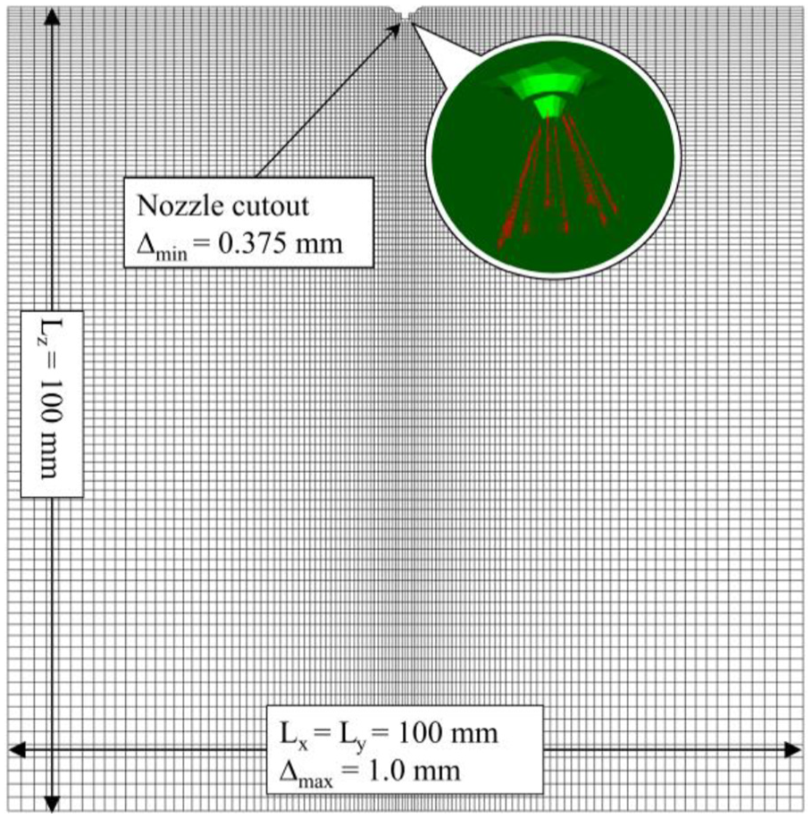
Cut plane of the cubic mesh with a nominal cell width of 1.0 mm. A nozzle cut-out approximating the geometry of the multi-hole injector is included to guide the air entrainment near nozzle exit, as the embedded sub-figure shows.

Figure 7 shows the liquid and vapor penetration results under the standard Spray G conditions. Also plotted are experimental data using Mie-scatter imaging and Schlieren from Sandia National Laboratory (SNL) and Istituto Motori.^57,58 For liquid penetrations shown in Figure 7, the results converge when the cell sizes are smaller or equal to 0.5 mm. The estimated liquid residence time is the same among all three meshes. The 1.0 mm mesh predicts slightly higher liquid penetration compared to the other two after 0.6 ms ASOI, but the difference is not significant, and the predicted trends follow each other closely. For the vapor penetrations shown in Figure 7, both 1.0 and 0.5 mm meshes predict very similar results throughout the simulation, and the 0.375 mm mesh predicts slightly higher vapor penetration after 0.5 ms ASOI. Results from all three meshes match the Schlieren data from Istituto Motori reasonably well, but fail to match the SNL data. 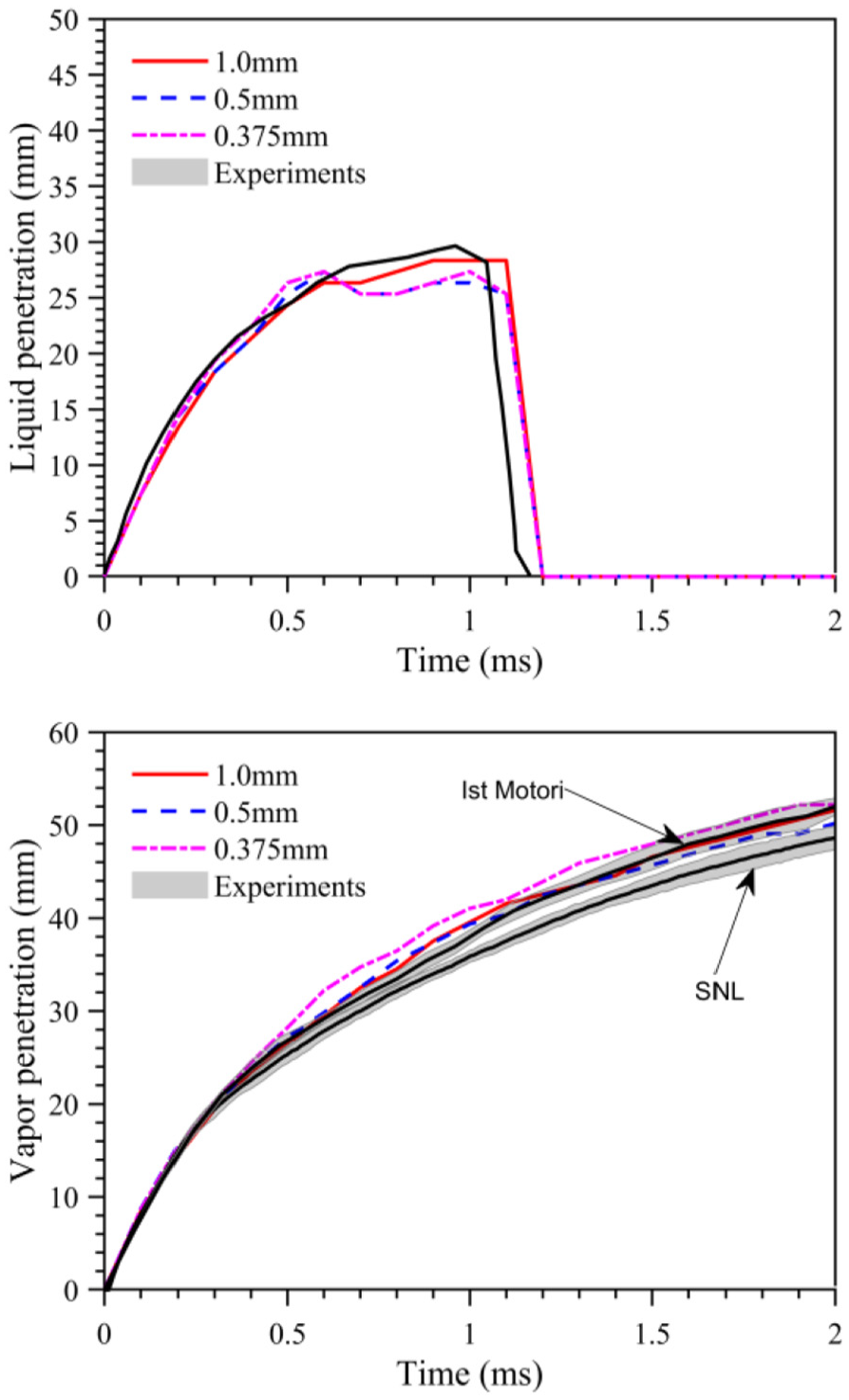Figure 8 presents the SGS turbulent kinetic energy, $k_{sgs}$ , along the plume centers at 0.5 ms ASOI. It is seen that $k_{sgs}$ is larger with finer mesh within 3 mm from the injector tip. This is expected since the liquid volume fraction increases as the cell size decreases, which leads to larger spray source term in the $k_{sgs}$ —transport equation and hence higher $k_{sgs}$ generation. The differences among three plotted curves become smaller at distances of 5 mm and further, implying that the SGS turbulence field is properly resolved. Overall, the LES results do not show great sensitivity to the mesh sizes. The 1.0 mm mesh is therefore used for the remaining part of this work due to its uniformity and reduced computational cost.

Figure 7.

Liquid and vapor penetration curves for case 1 (standard Spray G condition). The experimental data are plotted with the shaded area representing the 95% confidence levels. The simulation results are from single realizations for each mesh.

Figure 8.

Comparison of the SGS turbulent kinetic energy along plume centerlines for case 1. The results are given at t = 0.5 ms ASOI.

Results and discussion

Prior to the discussion of spray breakup modeling, the bag formation and bag growth processes are analyzed. Evaluation of the IAB model is then performed by comparing its predictions with experimental data and simulation results using the KH-RT model. Targeted spray characteristics include penetration rates, droplet velocity, and SMD profiles. Subsequently, further discussion focusing on the IAB breakup characteristics is provided. Finally, an attempt to correlate the optimal breakup model parameter values with the ambient conditions is made, and the found value is tested under a wide range of DISI spray conditions.

Analysis of the bag characteristics

Bag growth plays a crucial role in the bag breakup process as it determines the breakup length scale. To analyze the evolution of bag over time, initially spherical droplets are assumed to enter a constant flow field so that the initial We equals a specific value. The non-dimensional diameter ratios are then analyzed using equations (5)–(7). Available experimental data from Chou and Faeth,¹⁹ Krzeczkowski,¹⁴ and Kulkarni³⁶ are used for validation purpose. The measurements were carried out with different experimental setups and working fluids. A typical setup includes a droplet generator, a wind tunnel or a shock tube, and optical diagnostic systems for velocity and droplet size measurements.

Figure 9 presents the temporal evolution of measured and predicted cross-stream bag diameters at various We and Oh numbers. The scattered experimental data reported on x and y axes were normalized by the non-dimensional time, $T^{*}$ , and the initial droplet diameter, $d_{d 0}$ , respectively. For brevity, fluid properties and experimental setup employed in each study (e.g. droplet diameter and carrier phase velocity) are omitted. On each sub-figure, analytical results obtained using equations (5)–(7) are overlaid as solid lines. Figure 9 shows that all studies qualitatively agree with one another with increasing We number. In both experiments and predictions, the diameter ratio starts to increase slowly during a short period (t* < 0.6) after the droplet enters the disruptive gas field, indicating the transition from a spherical droplet to a relatively thin liquid disk. A liquid bag then forms at the center of the deforming disk and grows rapidly due to the pressure difference inside and outside the bag. The fast growth of the liquid bag also causes the thicker torus ring attached to the open end of the bag to expand in the cross-stream direction. Finally, after the bag rupture, the remaining torus ring continues to expand with a constant velocity until it breaks due to RT instabilities. Note that the rate of cross-stream expansion is the largest when the bag is present, which is in agreement with the findings in Chou and Faeth.¹⁹ The diameter ratios in Figure 9(e) differ between experiments and predictions. This is attributed to the difficulties in experimental measurements. While the torus ring is assumed to be of circular shape in equations (5)–(7), it is often heavily curled or distorted in experiments, especially at relatively larger We number.^19,23 Results also show that the droplet Oh number has little effect on the bag growth for the Oh range considered in this analysis.

Figure 9.

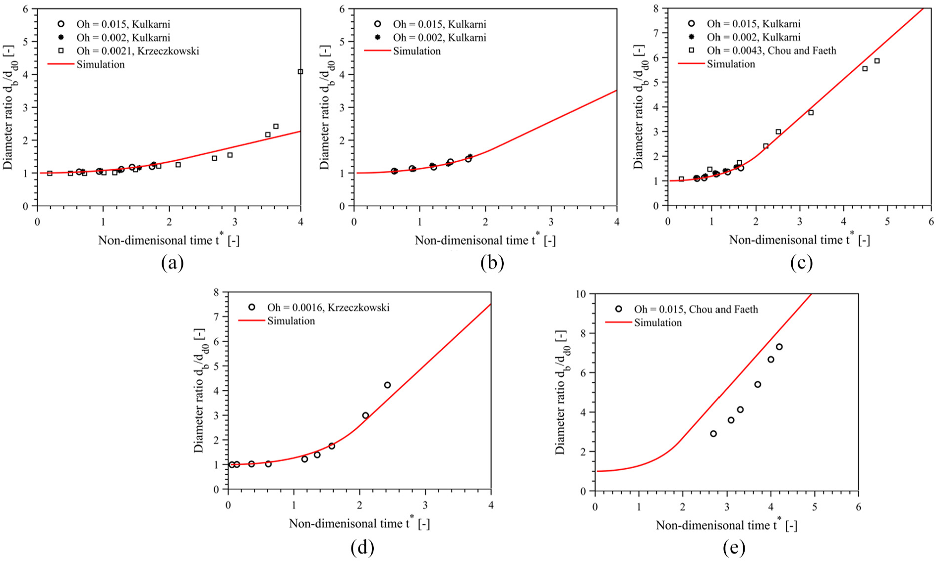
Measured and predicted cross-stream diameters at various We and Oh numbers: (a) We₁ = 13, (b) We₁ = 14, (c) We₁ = 15, (d) We₁ = 18, and (e) We₁ = 20. The data reported on both x and y axes have been normalized by the non-dimensional breakup time, $T^{*}$ , and the initial droplet diameter, $d_{d 0}$ , respectively.

It is important to understand how the bag develops beyond the scope of experiments illustrated in Figure 9. Therefore, the predicted cross-stream diameter ratios for We from 6 to 56, covering a wide range of the bag and bag–stamen breakup, are computed and plotted in Figure 10. On each curve, the onset time of bag rupture is also overlaid as an asterisk. At $We = 6$ , the droplet undergoes deformation with no bag develops on its surface. Further increasing of We promotes a rapidly expanding liquid bag as expected. However, the onset time of bag rupture decreases as We increases, leaving a shorter time for the torus ring to gain momentum from the growing bag. The competitive contributions from the above two factors give a complex behavior of the cross-stream diameter ratio. Before the bag ruptures, the growth rate increases monotonically with We, but the difference becomes less noticeable at higher We number. After the bag ruptures, the liquid torus expands with a constant rate, whose value initially increases then decreases with larger We. This behavior confirms that the size of the liquid torus is not excessively larger than the initial droplet diameter. It also suggests that the bag structure is unlikely to develop at very high We numbers.

Figure 10.

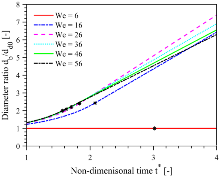
Predicted cross-stream diameter ratio as a function of non-dimensional time at various We. Asterisks are overlaid on each curve to illustrate the onset time of bag rupture.

Initial calibration: liquid and vapor penetration curves

Both the IAB and the KH-RT models were calibrated at the baseline DISI conditions illustrated in Figure 5. Liquid and vapor penetrations were selected as the target spray characteristics. Two IAB model parameters, namely, B₁ and α, were adjusted using a Monte Carlo approach to obtain optimal predictions compared to the measured penetration curves. The same process was conducted for the KH-RT model using the calibration of three model parameters: B₁, C_b, and C_τ. Although it requires more efforts to obtain the optimum compared to the IAB model, it is deemed necessary since adjusting B₁ and C_b will not match both the liquid and vapor penetrations, as reported by Van Dam and Rutland.³⁴ Predicted liquid and vapor penetrations are plotted in Figures 11 –14 for cases 1–4, respectively. Available experimental data for the penetration measurements are also plotted on each figure, with the shaded area representing the 95% confidence levels.

Figure 11.

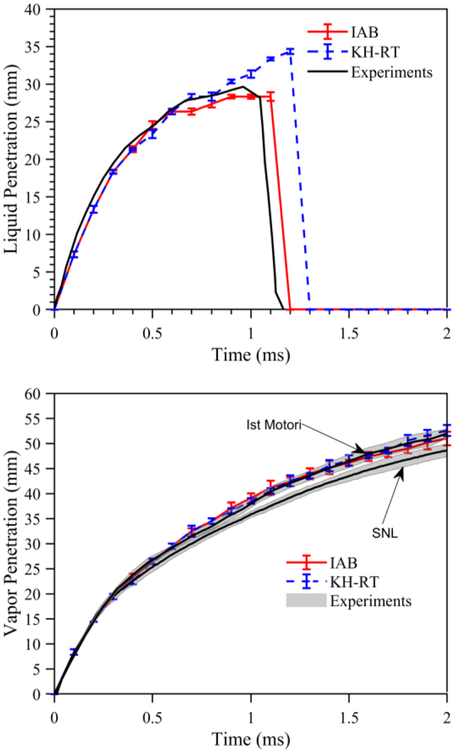
Liquid and vapor penetration curves for case 1 (standard Spray G condition). The predicted results are ensemble-averaged over five realizations and plotted with error bars representing the standard deviations. The measured vapor penetrations are plotted with the shaded area representing the 95% confidence levels.

Figure 12.

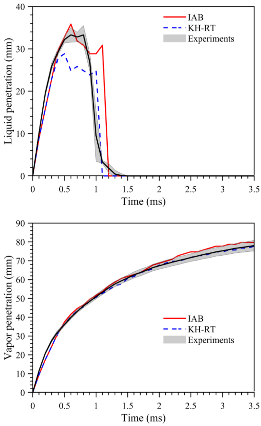
Liquid and vapor penetration curves for case 2 (GM DISI sprays at 800 K, 3.0 kg/m³). The experimental data are plotted with the shaded area representing 95% confidence levels. The simulations results are from single realizations.

Figure 13.

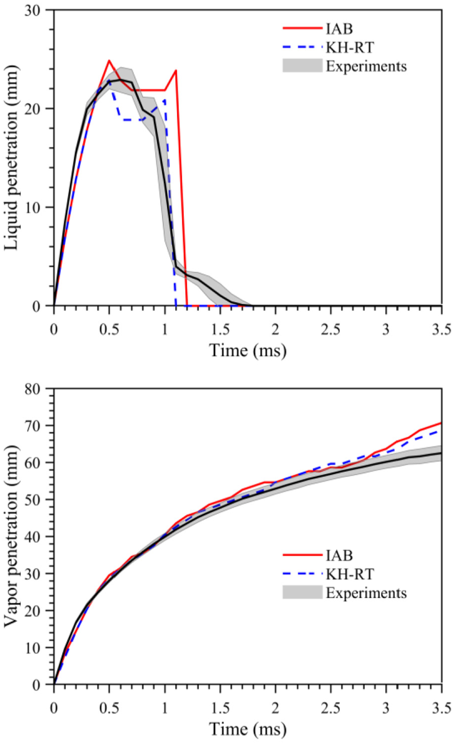
Liquid and vapor penetration curves for case 3 (GM DISI sprays at 800 K, 6.0 kg/m³). The experimental data are plotted with the shaded area representing the 95% confidence levels. The simulations results are from single realizations.

Figure 14.

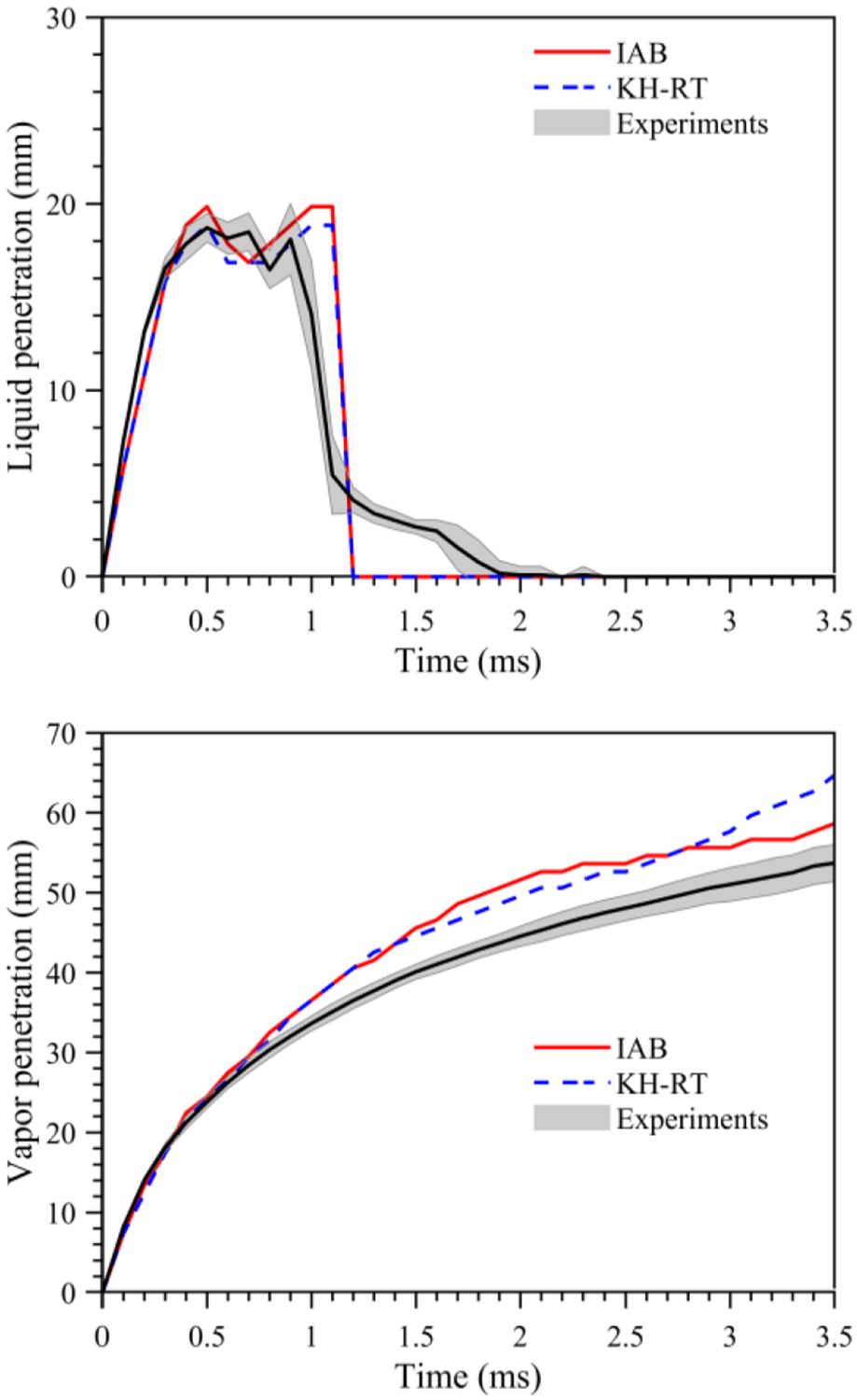
Liquid and vapor penetration curves for case 4 (GM DISI sprays at 800 K, 9.0 kg/m³).The experimental data are plotted with the shaded area representing the 95% confidence levels. The simulations results are from single realizations.

Figure 11 presents the penetration curves for case 1, the standard Spray G conditions. Numerical results averaged over five realizations are plotted with the corresponding standard deviations as error bars. Both the liquid and vapor penetrations match the measured curves very well during the early period of injection (t < 0.2 ms ASOI). Then, liquid penetrations become parabolic due to droplet breakup and aerodynamic drag after approximately 0.2 ms ASOI. Simulations show more variability during the quasi-steady stage of injection (0.5 < t < 0.7 ms ASOI). The maximum standard deviations for the liquid penetrations are 0.6 and 0.5 mm for the IAB and KH-RT models, respectively, indicating that both models are insensitive to the random number seed in the injection model. As one may expect, only by changing the random number seed is not sufficient to represent the uncertainties in spray and ambient conditions. Indeed, UQ with proper variations in the boundary conditions is needed to obtain realistic results.⁵³ The negligible standard deviations also suggest that the discrete Lagrangian phase has reached a statistical convergence with the current setup of total injected parcels. Better matching to the experimental data is given by the IAB model during this period. The liquid penetration eventually goes to zero due to evaporation. The timing of this transition is estimated to be around 1.2 ms ASOI by Mie-scatter imaging measurement,⁵⁷ which is well captured by the IAB model. The liquid length is measured to be 30 mm. The IAB model predictions follow the measurements data closely with a liquid length of 28.3 mm. The KH-RT model, however, predicts the spray to penetrate further downstream until it reaches a liquid length of 35 mm.

The experimental vapor penetrations from SNL and Istituto Motori are plotted in Figure 11. Even though both groups use the same injector at the same nominal spray conditions, the exact setup differs. For transient sprays, a small variation in the initial and boundary conditions can result in large changes in penetration rates at later times. Figure 11 shows that the measured vapor penetrations start to deviate from each other after 0.3 ms ASOI. The deviation continues to increase until about 1.0 ms ASOI, after which the measured curves become parallel to each other. The maximum vapor penetrations are 48.6 and 52 mm for the SNL and Istituto Motori measurements, respectively. The predicted vapor penetrations match the Istituto Motori measurements very well. Small differences are observed between the predicted results. However, both models over-predict the penetration rates compared to the SNL data after 0.5 ms ASOI. The maximum standard deviations are 1.3 and 1.1 mm for the IAB and KH-RT models, respectively. Compared to the mean penetrations at 2.0 ms ASOI, the standard deviations are rather subtle. Therefore, in the following discussion, only single realizations are performed for the GM DISI sprays.

Figures 12 –14 present the measured and predicted penetration curves for cases 2–4 (GM DISI conditions of 800 K and 3.0, 6.0, and 9.0 kg/m³, respectively). Again, simulations with the IAB model match the experimental data very well at all three conditions for liquid penetration. Similar to case 1, the spray structures reach quasi-steady states around 0.5 ms ASOI. The liquid length is well captured by the IAB model as well. On the contrary, KH-RT model under-predicts the liquid penetration at both 3.0 and 6.0 kg/m³. The effects of changing ambient density on liquid penetration at the temperature of 800 K are also illustrated in Figures 12 –14. Comparing with the result at the ambient density of 3.0 kg/m³, the liquid length decreases by about 33% and 42% at higher densities of 6.0 and 9.0 kg/m³, respectively. The reduction in liquid length at higher ambient density is expected since the aerodynamic drag increases as well. The measured liquid penetrations also show a gradually retracting liquid tip after the end of injection. This behavior is likely attributed to nozzle dribble from the sac volume after the injection or light reflection by the nozzle tip. Unfortunately, present LES framework is unable to simulate dribble from the nozzle sac volume due to a lack of internal flow modeling.

The predicted vapor penetrations in Figures 12 and 13 match the experimental data to within 95% confidence levels except at the very end of simulation for the 6.0 kg/m³ case, where a sudden increase is observed with both models. This is caused by vapor protrusion along the injector axis as documented in a recent UQ study by the authors.⁵³ The reason of vapor protrusion is unknown at this time, but it is unlikely caused by the breakup models as the timing (3.5 ms ASOI) is about four times larger than the injection duration. In Figure 14, both models tend to over-predict the vapor penetration just before the end of injection. Like the liquid phase, increasing ambient density also causes a reduction in vapor penetration. Overall, the predicted vapor penetrations show little difference between the KH-RT and the IAB model predictions.

The IAB model parameter values from the optimal calibration for baseline cases 1–4 are listed in Table 4. The difference observed in the α values among all four cases is subtle. However, B₁ values are highly different between Spray G and GM DISI sprays. Indeed, B₁ is given a variety of values as reported in Reitz and Beale,³⁸ Ricart et al.,⁴⁰ Van Dam and Rutland,⁷¹ and Brulatout.⁷² The rather large B₁ range owes to the fact that the initial KH unstable waves rely heavily on the fuel properties, injector geometry, and near-nozzle air entrainment. The rather close α values indicate that the baseline conditions may share the same density ratio dependency of the breakup length. In support of this statement, the nominal breakup length along the plume centerlines at the baseline conditions was calculated using equation (4) and results are shown in Figure 15. Also plotted are the breakup lengths calculated using equation (3) for the optimal KH-RT simulation results discussed previously. The corresponding model parameter values are listed in Table 6 in Appendix 2. The final combination of KH-RT parameter values from the study of Van Dam are also listed in Table 6 for comparison purpose.³⁴ Note that the plotted results are computed using the nominal ambient densities depicted in Figure 5. In simulations, the ambient density will increase due to evaporation, which in turn leads to reduced breakup length.

Table 4.

IAB breakup model parameter values at ECN Spray G and GM DISI spray conditions.

Case number	Ambient density (kg/m³)	Ambient temperature (K)	α in equation (4)	B₁ in the IAB model
1	3.5	573	0.92	30
2	3.0	800	0.89	50
3	6.0	800	0.93	50
4	9.0	800	0.93	50

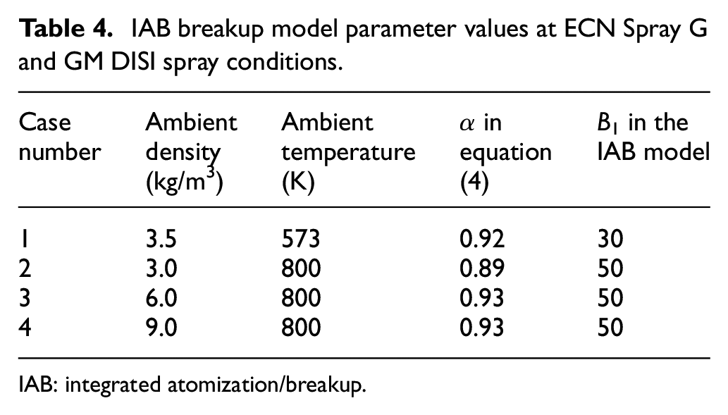
IAB: integrated atomization/breakup.

Figure 15.

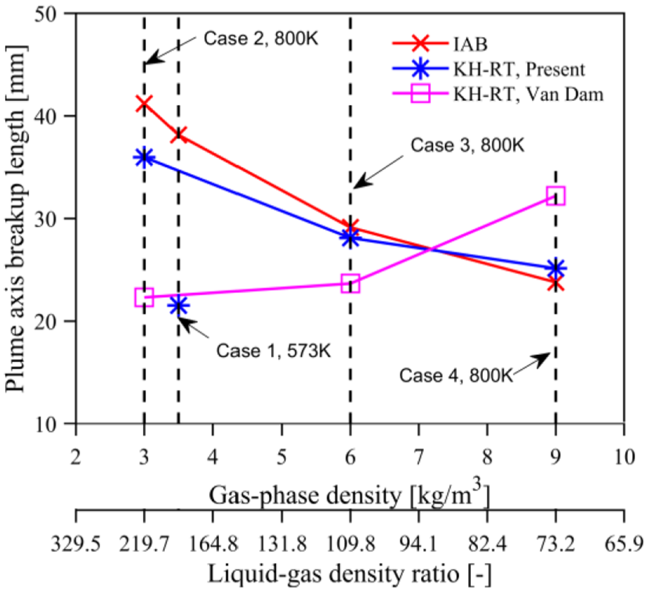
Nominal breakup length along the plume centerlines at the baseline conditions.

Figure 15 shows that as the ambient density increases, the liquid-gas density ratio decreases, which in turn leads to a reduced breakup length in the IAB model. This trend is consistent with the expectation that higher ambient density leads to reduced breakup length. However, the breakup length adopted by the KH-RT model exhibits opposite trends between this work and Van Dam and Rutland³⁴ for cases 2–4. Van Dam and Rutland demonstrated that the breakup length increases as the density ratio decreases, while in this work, the breakup length is shown to decrease at higher gas-phase densities. This opposite relationship can be explained by the different revisions of the KH-RT model between this work and Van Dam and Rutland.³⁴ In this work, the RT breakup model is only activated once a parcel travels beyond the pre-calculated breakup length. The child droplet sizes after breakup are set to be the RT wavelength, $Λ_{RT}$ . In contrast, the KH-RT model revised by Beale and Reitz³⁸ was used by Van Dam and Rutland,³⁴ in which the RT breakup is also activated even if the parcel is located within the breakup length. However, this generally results in faster breakup, and to compensate for that, the RT breakup time constant, $C_{τ}$ , was set to 9.0 for parcels within the breakup length. In addition, the child droplet sizes from RT breakup are selected from a Rosin–Rammler distribution. In general, both KH-RT revisions struggle to predict accurate penetration curves under the GM DISI conditions, as discussed in the previous section and Van Dam and Rutland.³⁴ Moreover, the breakup length obtained from the optimal KH-RT simulations for case 1 does not correlate with the other three cases.

Droplet velocity and SMD profiles

After the initial calibration targeted at penetration curves, more rigorous validation of the models is conducted focusing on the droplet velocity and SMD distributions. Data are sampled at the standard Spray G condition in the radial direction through the plume centers at 15 mm axial position, a location where the experimental data are available. The ensemble-averaged simulation results of all eight plumes and five realizations at two selected timings, 0.5 ms and 1.5 ms ASOI, are plotted with PDI data in Figure 16. Simulation results are plotted with the standard deviations computed over 40 samples. The experimental data are plotted with the mean values only. At 0.5 ms ASOI, where the injection reaches quasi-steady state, the predicted droplet axial velocities show little differences and they both match the experimental data very well, except for the 10 mm radial position where both models under-predict the maximum axial velocity. The measured local maximum is 50 m/s, while the predicted ones with the KH-RT and IAB models are 40 and 42 m/s, respectively. This implies that the IAB model does predict slightly better axial velocity than the KH-RT model, though the improvement is minor. As for the SMD profiles, an immediate observation is that the simulation results extend to the outer edge of the spray plume. The over-prediction of SMD distributions at the outer edge corresponds to a region of relatively large droplets with low speed. Note that no experimental data are available at radial locations farther than 14 mm, making it harder to evaluate the models. However, the IAB model gives smoother SMD distribution compared to the KH-RT model. The maximum SMD predicted by the KH-RT model is 42 µm, while the one given by the IAB model is 16 µm.

Figure 16.

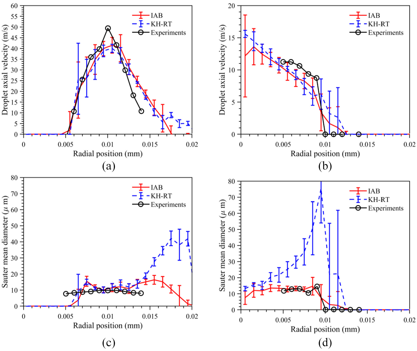
Plume-centered radial distribution of the axial droplet velocity and droplet SMD for case 1. (a) Axial droplet velocity: 0.5 ms ASOI. (b) Axial droplet velocity: 1.5 ms ASOI. (c) SMD: 0.5 ms ASOI. (d) SMD: 1.5 ms ASOI. Results are sampled at z = 15 mm, and 0.5 and 1.5 ms ASOI. Predicted results are averaged over eight plumes and five realizations and plotted with corresponding standard deviations.

At 1.5 ms ASOI, the residual droplets can no longer be detected by the LOS spray visualization measurements, as evidenced by Figure 11, where both measured and predicted liquid penetrations are zeros. However, droplets can still be captured by the PDI system. As Figure 16(b) and (d) shows, the predicted droplet velocity and SMD distributions by both models show moderate differences, especially the SMD distributions at 9 mm radial position. The predicted SMD by the IAB model is around 10 µm, which is in agreement with the measured data. In the case of KH-RT model, the local maximum is predicted to be 75 µm. Better agreement with the experiments is given by the IAB model, despite the relatively large standard deviations at 1.5 ms ASOI. This improvement owes to the fact that droplet velocities are relatively low at 1.5 ms ASOI, leading most of the residual droplets into the bag and deformation breakup regimes, as will be further elaborated later. The bag sub-model is responsible for the breakup description of remaining droplets that are still undergoing breakup process.

Characteristics of the IAB model

More insights into the IAB model can be gained by examining the occurrence percentage of each sub-model for the baseline cases. The occurrence percentage is defined as the ratio of the number of liquid parcels driven by each sub-model to the total number of existing liquid parcels. 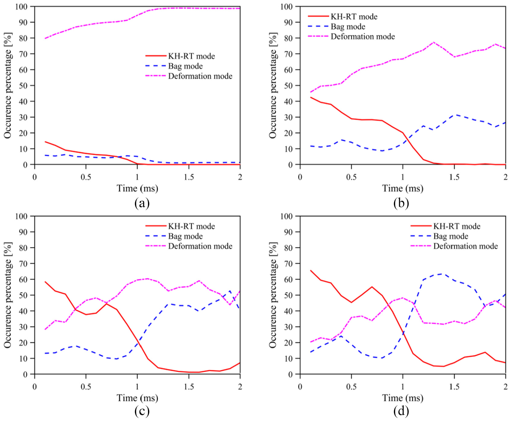Temporal evolution of these quantities are shown in Figure 17, where it is found that a decrease in either the ambient temperature or density leads more parcels with We smaller than $W e_{crit}$ , making them fall within oscillation/deformation regime. As the ambient temperature increases, the evaporation rate increases as well, which in turn reduces the life span of small droplets and hence the occurrence percentage of deformation mode. We number increases with the ambient density, leading to more droplets in the plume-sheet thinning, sheet-thinning, and catastrophic breakup regimes.

Figure 17.

Occurrence percentage of the IAB breakup sub-models for baseline cases. (a) Case 1, 573 K, 3.5 kg/m³. (b) Case 2, 800 K, 3.0 kg/m³. (c) Case 3, 800 K, 6.0 kg/m³. (d) Case 4, 800 K, 9.0 kg/m³.

Figure 17 shows that the occurrence percentages of the deformation mode are already large at 0.1 ms ASOI. About 80% of fuel parcels in the domain are driven by this mode for the moderate-temperature case 1. This is caused by the substantial amount of micro-size child droplets resulting from KH-breakup. Moving to the high-temperature GM DISI conditions at the same time, the percentages reduce to 46%, 28%, and 20% for the ambient densities of 3.0, 6.0, and 9.0 kg/m³, respectively. This trend is accompanied by the observation that the KH-RT breakup mode drives more parcels at higher densities. This is expected since droplet We number increases proportionally with the ambient density. In general, the occurrence percentages of KH-RT mode decrease as time proceeds, though they seem to bump up around 0.5 ms ASOI for cases 3 and 4. It is also noted that the KH-RT mode drives more parcels than the bag mode for case 1 before the injection ends at 0.78 ms ASOI. The crossover happens even later for the high-temperature GM DISI conditions. While the injection ends at 0.865 ms ASOI, the bag mode only begins to surpass the KH-RT mode at about 1.0 ms ASOI. The relative dominance of bag mode over KH-RT after the injection also explains why the SMD and velocity predictions of the IAB model are improved at 1.5 ms ASOI, as shown in Figure 16.

As discussed previously, a bi-modal distribution is expected for the bag breakup.^28,36 However, the number of child droplets from bag rupture may overwhelmingly outnumber that from the liquid torus breakup, making it difficult for this distribution to be observed in experiments.³⁶ In simulations with the parcel approach, this limitation can be easily overcome if results are processed based on fuel parcels, as opposed to the fuel droplets discussed in Figure 16. Recall that a parcel is an ensemble of several maybe hundreds of droplets with same properties. In the bag breakup model, child droplets from bag rupture and torus breakup are enclosed by two separate parcels. Figure 18 shows the PDFs of parcel diameters at 1.1 ms ASOI for baselines cases. Results obtained using the IAB and KH-RT models are plotted on the left and right sub-figures, respectively. Note that all remaining parcels in Figure 18(a) are either driven by the deformation mode or the bag mode since the occurrence percentage of the KH-RT mode is less than 1%, as shown in Figure 17(a). It can be seen that most residual parcels are smaller than 25 µm, with the peaks located at around 10 µm. These small parcels likely lie within the deformation regime where parcels no longer break. Moving to larger parcels, two peaks in PDFs are seen in results from the IAB model. The peaks in the middle are likely associated with the liquid torus rings after bag rupture, while the peaks on the right correspond to the growing bag. This observation supports the bi-modal droplet size distribution. However, the KH-RT model does not show such behavior at larger parcel diameters, as shown in Figure 18(b).

Figure 18.

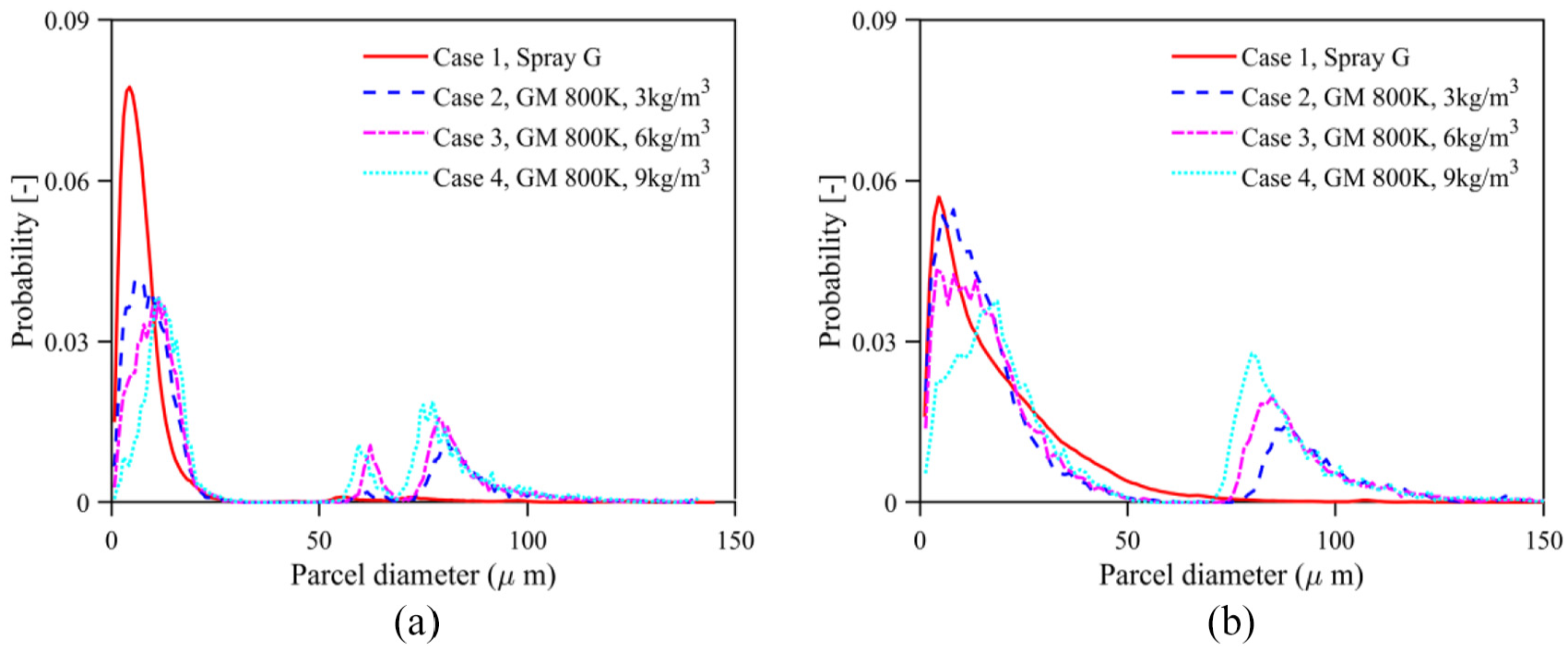
PDF of parcel diameters at 1.1 ms ASOI for test cases 1–4, using (a) IAB and (b) KH-RT models.

Application to other DISI conditions

Additional evaluations of the IAB model were done by extending the test matrix to more ambient temperature conditions for GM DISI sprays. Rather than providing the optimal calibration results for each case, we intended to develop a unified set of model parameters to reduce the efforts needed for calibrating the IAB model at different DISI spray conditions. Recall that α values for the density conditions listed in Table 4 are quite close to each other. Assuming the value of α is a constant for DISI sprays with a specific type of fuel, then a reasonable estimation can be made by averaging the α values in Table 4. However, no effort is made to correlate B₁ with ambient conditions, since its value appears to be highly dependent on the injector geometry and near-nozzle air entrainment.

Figures 19 and 20 present the liquid and vapor penetration curves for all GM DISI temperature and density conditions listed in Table 3. Simulation results were taken from single realizations with the IAB model parameters α = 0.92 and B₁ = 50. Experimental data were the average of 25 duplicate measurements. The left columns show the liquid penetration curves, and the right ones show the vapor penetration results. The top rows show results at 3.0 kg/m³, and the following two rows show the results at 6.0 and 9.0 kg/m³, respectively. For clarity of presentation, experimental data are only plotted with the ensemble-averaged values.

Figure 19.

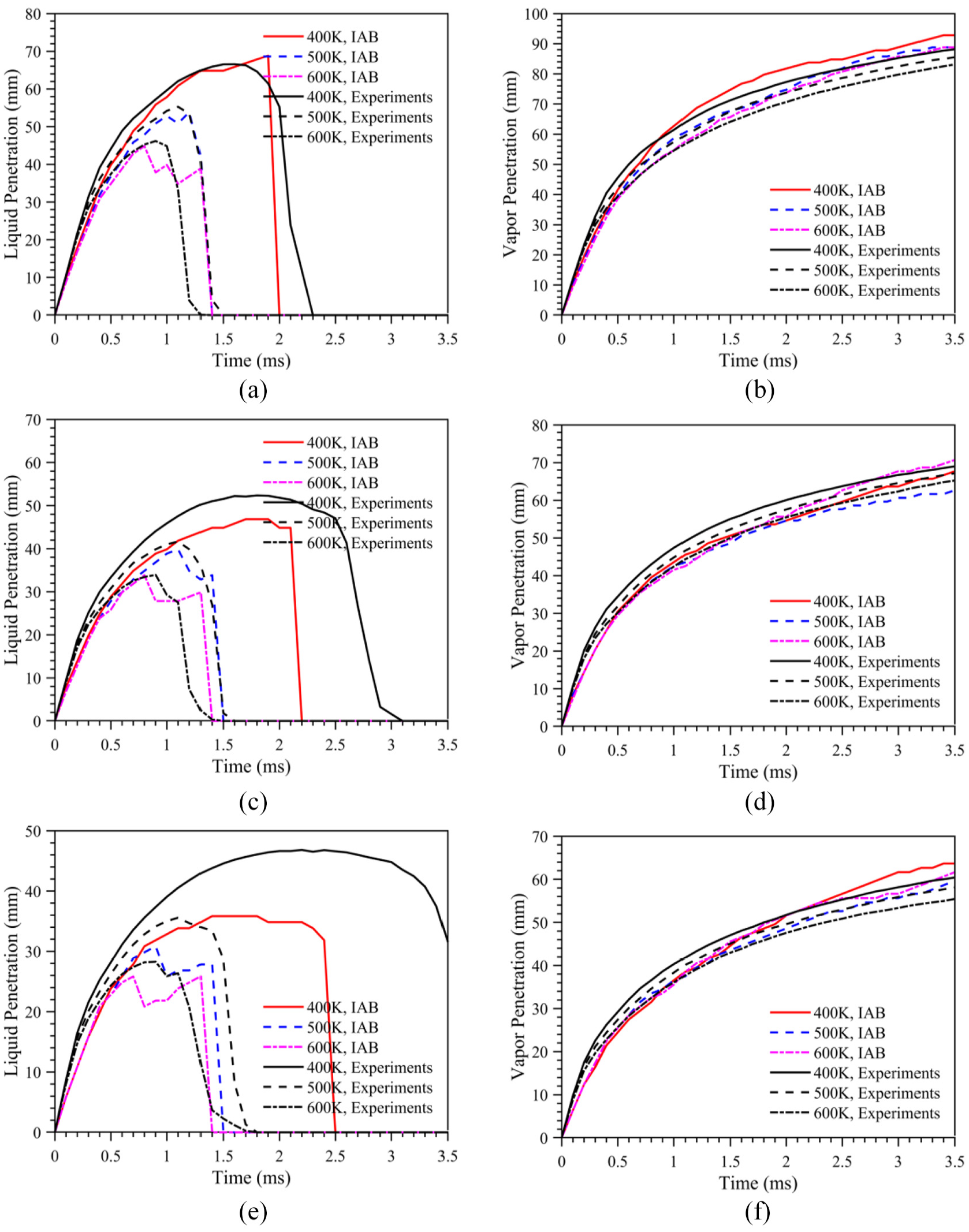
Comparison of penetration curves between simulations and experiments at GM DISI spray conditions of 400–600 K: (a) liquid penetration, ρ_a = 3.0 kg/m³; (b) vapor penetration, ρ_a = 3.0 kg/m³; (c) liquid penetration, ρ_a = 6.0 kg/m³; (d) vapor penetration, ρ_a = 6.0 kg/m³; (e) liquid penetration, ρ_a = 9.0 kg/m³; and (f) vapor penetration, ρ_a = 9.0 kg/m³. Experimental results are averaged over 25 measurements. Simulations results are taken from single realizations.

Figure 20.

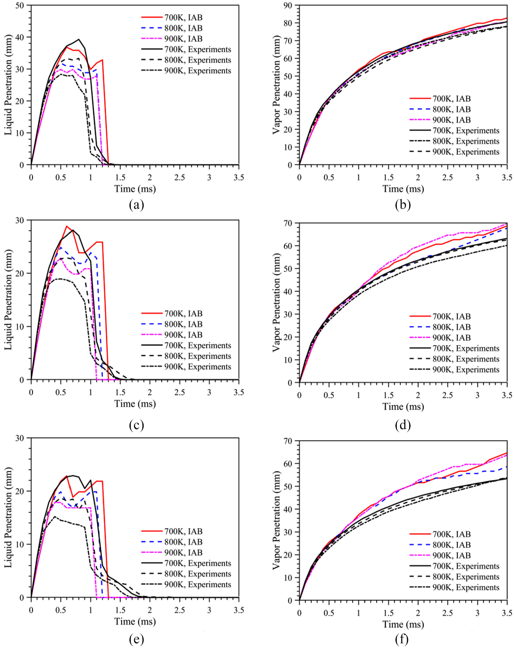
Comparison of penetration curves between simulations and experiments at GM DISI spray conditions of 700–900 K: (a) liquid penetration, ρ_a = 3.0 kg/m³; (b) vapor penetration, ρ_a = 3.0 kg/m³; (c) liquid penetration, ρ_a = 6.0 kg/m³; (d) vapor penetration, ρ_a = 6.0 kg/m³; (e) liquid penetration, ρ_a = 9.0 kg/m³; and (f) vapor penetration, ρ_a = 9.0 kg/m³. Experimental results are averaged over 25 measurements. Simulations results are taken from single realizations.

A general trend found in Figures 19 and 20 is that higher ambient density leads to reduced liquid length due to the enhanced air entrainment, increased aerodynamic drag, and possibly faster droplet breakup. In Figure 19, the density impact is more pronounced at 400 K compared to 500 K and higher. The liquid residence time also shows the largest difference at 400 K, in which an increase in the ambient density will lead to longer liquid residence time. This is expected since the pressure must be elevated to keep the ambient density constant, and the elevation in ambient pressure suppresses evaporation, hence increases the life span of small droplets. The simulations are able to reproduce the shape of the experimental curve at 3 kg/m³, but fail to even capture the general trends at higher densities. The comparison is more favorable at elevated temperatures and reduced densities, where both the liquid length and residence time are well predicted. In Figure 20, the predicted liquid penetration curves match the experimental data reasonably well with the exception of 900 K at 6.0 and 9.0 kg/m³, where the penetrations are over-predicted. Despite the magnitudes of liquid penetrations being off at these two conditions, the trend and the liquid residence time are still well captured.

The predicted vapor penetration curves in Figure 19 agree reasonably well with the Schlieren measurements. At 400 K, the vapor penetration results are under-predicted during the initial period of injection at all three density conditions. One possible reason is the identical spray initial and boundary conditions at the nozzle exit at each density condition. While in experiments the ambient temperature and pressure influence the spray behaviors such as the plume cone angle and near nozzle air entrainment, in simulations the spray boundary conditions are kept unchanged among all cases since the primary goal of this test is to see if the IAB model can perform well under conditions beyond the scope of cases 1–4. In Figure 20 at 800 K, the predicted vapor penetrations match the experimental data quite well at 3.0 and 6.0 kg/m³, even though they are not the calibrated results since the parameter α in equation (4) is changed. At 9.0 kg/m³, the predicted vapor penetration results are somewhat discouraging. One possible reason is the extra momentum gained from the over-penetrating liquid droplets as shown in the left columns. Other factors such as the turbulence model can also come into play.

The liquid length and liquid residence time are perhaps two important macroscopic spray characteristics in DISI sprays. In general, the liquid length needs to be accurately captured since it affects the wall-impingement and hence the following mixing and combustion processes. The liquid residence time is also of importance as residual droplets can be a potential source of soot. Therefore, a comparison of these two quantities is extracted from Figures 19 and 20 and plotted in Figures 21 and 22. While the calculation of liquid length is straightforward, the definition of liquid residence time is somewhat vague. In experiments, the liquid residence time is defined as the time required for the penetration to fall to half the maximum due to vaporization.⁴⁸ In simulations, however, the residence time is defined as the time when the liquid penetration falls to zero. The difference caused by this discrepancy is expected to be negligible providing the liquid penetration falls rapidly back to zero in the simulations.

Figure 21.

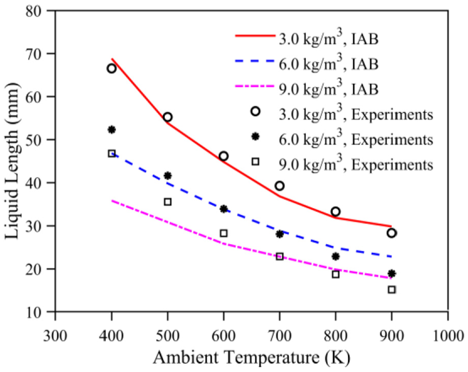
Liquid length as a function of ambient temperature. Symbols represent the measured data from Mie-scatter imaging. The continuous curves represent numerical results using the IAB model.

Figure 22.

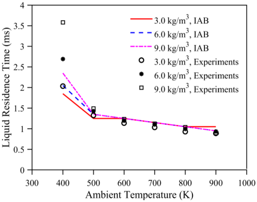
Liquid resident time as a function of ambient temperature. Symbols represent the measured data from Mie-scatter imaging. The continuous curves represent numerical results using the IAB model.

In Figure 21, the predicted liquid length results are plotted as functions of ambient temperature for the three ambient densities. Experimental data from the Mie-scatter imaging are also plotted as symbols for comparison. It is seen that the predictions match the experimental data very well at 3.0 kg/m³. At 6.0 kg/m³, the agreement is quite good as well except at 400 and 900 K, where successful predictions are not achieved. At 9.0 kg/m³, the simulation results only match the experimental data at 700 and 800 K. However, the general trend of reduced liquid length with increasing ambient temperature is still captured by the model.

The results of liquid residence time are shown in Figure 22. First, it is seen that the liquid residence time is independent of the ambient density for temperatures of 500 K and higher. This implies that the ambient air provides enough energy to vaporize the fuel regardless of changes in the ambient density. At 400 K, the measured liquid residence times change with density, indicating that this independence no longer stands. In general, higher density enhances the air entrainment and hence increases the energy available for evaporation. However, evaporation is suppressed at increased density, since the pressure must be elevated given the temperature is unchanged. It can be seen that the liquid residence time increases drastically as the density increases, suggesting the evaporation plays a more important role than air entrainment. As Figure 22 shows, the measured liquid residence time increases by 32% and 76% when the ambient density increases from 3 to 6 and 9 kg/m³, respectively. However, the predicted residence time only increases by 11% and 26% for the same changes. The lack of sensitivity to the density change at 400 K suggests that the evaporation rate is over-predicted at higher density cases. This can be a result of either increased droplet area-to-volume ratio caused by accelerated breakup modeling, or inaccurate phase-change rate by the evaporation model, or even a combination of both factors. At the low-temperature condition of 400 K, high pressure is not required to maintain the densities at 3, 6, or 9 kg/m³. The near-nozzle air entrainment is therefore expected to be not as strong as the other conditions. This will result in a smaller plume angle and possibly weaker KH disturbance levels at the nozzle exit. Since the value of B₁ was calibrated at much higher temperature and pressure conditions, keeping B₁ unchanged is expected to give accelerated breakup.

Summary and conclusion

Direct injection diesel and gasoline sprays share many similarities in terms of the injection system and spray pattern, yet there are many differences in the thermophysical properties and operating conditions. In the LES of DISI gasoline sprays, in order to more precisely describe the fuel–air mixing, one may need to take into account the effects of these differences on liquid atomization and breakup, which are mainly expressed as different breakup mechanisms of fuel droplets. In this article, an IAB model tailored for DISI gasoline sprays is presented. In the IAB model, atomization of liquid jet near the nozzle exit and the subsequent breakup of liquid fragments and droplets are treated as indistinguishable processes, and the “blob” approach is adopted to represent the liquid fuel regardless of its physical appearance (jet, ligament, or droplet). The breakup simulation has been divided into two regimes, namely, the bag/bag–stamen breakup regime, and the high We number regime. In the first regime, a phenomenological bag breakup model has been developed by the authors to track the breakup process. In the second regime, the breakup modeling is based on the KH-RT model by Reitz and coworkers with a revised breakup length concept.

The initial calibration has been carried out by adjusting the model parameter values to obtain the optimal matching of penetration curves between LES predictions and experiments. The standard Spray G condition defined by ECN and the spray measurements conducted by GM at the ambient temperature of 800 K and three densities of 3.0, 6.0, and 9.0 kg/m³ were used as four baseline cases. The optimal calibration of the KH-RT model has also been conducted and results were compared against the experiments and IAB model predictions. It was shown that the IAB model gives generally better agreement than the KH-RT model at all conditions discussed. The improvements were minor considering both models have been calibrated to give the best-matching results. However, further analysis of the breakup length reveals that the KH-RT model may not fully capture the atomization/breakup processes of DISI sprays. The KH-RT model also requires more efforts to calibrate, and the results may yield different trends of the characteristic breakup length depending on the implementations. However, the IAB model has an overall good performance among the four baseline cases and the resulting breakup lengths meet the expectation that higher ambient density leads to decreased breakup length.

The model has been further assessed by comparing the predicted droplet velocity and SMD distributions with PDI measurements at the standard Spray G condition. It is shown that the IAB model improves the predictions of droplet velocity and SMD distributions during and after the injection, especially in later times. Analysis of the occurrence percentage of each sub-models reveals that the KH-RT sub-model drives more parcels than the bag breakup model before the end of injection. However, the bag breakup mode becomes the dominant mechanism in later times. This is considered to be an important improvement over the KH-RT model since large residual droplets after the end of injection may be a potential source of soot emissions, and hence their breakup needs to be accurately modeled.

An effort has been made to unify the model parameters across the four baseline DISI conditions, and the given parameter values have been used to test the model performance at more GM DISI spray conditions. Changes in ambient temperature and density were studied. The results agree favorably with the experimental measurements, with some discrepancies at the lowest temperature of 400 K that can be explained. In most cases, the agreement is generally good considering that the model parameters were not tuned specifically for individual cases.

It is generally accepted that breakup models coupled with accurate spray boundary conditions and even the internal flow characterization are important for accurate prediction of spray behavior in direct-injection engines. For DISI sprays, the relatively small L/D ratios and volatile fuel components can lead to very complex internal turbulent flows and phase-change phenomena such as cavitation and flash boiling. This article presents a rather promising breakup model for DISI sprays. Future work will be focused on incorporating more physically representative sub-models to initialize the spray parcels at the nozzle exit and hence to improve the predictions at low-temperature conditions for GM DISI sprays.

Footnotes

Appendix 1

Appendix 2 Acknowledgements

The authors thank the UW–Madison High Throughput Computing for providing computer resources used to obtain the results presented in this publication.

Declaration of conflicting interests

The author(s) declared no potential conflicts of interest with respect to the research, authorship, and/or publication of this article.

Funding

The author(s) disclosed receipt of the following financial support for the research, authorship, and/or publication of this article: This work was supported by the Wisconsin Engine Research Consultants, LLC, and by the FUELCOM II collaborative project between King Abdullah University of Science and Technology and Saudi Aramco Oil Co.

ORCID iD

Hongjiang Li

References

Zhao

Lai

M-C

Harrington

. Automotive spark-ignited direct-injection gasoline engines. Prog Energy Combust Sci 1999; 25: 437–562.

Mitroglou

Nouri

Arcoumanis

. Spray structure from double fuel injection in multihole injectors for gasoline direct-injection engines. At Sprays 2009; 19: 529–545.

Kawaharada

Sakaguchi

Ueki

Ishida

. Effect of injection pressure on droplet behavior inside diesel fuel sprays. SAE technical paper 2015-01-1841, 2015.

Baumgarten

. Mixture formation in internal combustion engine. Berlin and Heidelberg: Springer.

Gorokhovski

Herrmann

. Modeling primary atomization. Annu Rev Fluid Mech 2008; 40: 343–366.

Lévy

Amara

Champoussin

J-C

. Simulation of a diesel jet assumed fully atomized at the nozzle exit. SAE technical paper 981067, 1998.

Huh

Gosman

. A phenomenological model of diesel spray atomization. In: Proceedings of international conference on multiphase flows, Tsukuba, Japan, 24–27 September 1991.

Arcoumanis

Gavaises

French

. Effect of fuel injection processes on the structure of diesel sprays. SAE technical paper 970799, 1997.

Amsden

O’Rourke

Butler

. KIVA-II: a computer program for chemically reactive flows with sprays, 1989, https://www.osti.gov/biblio/6228444-kiva-ii-computer-program-chemically-reactive-flows-sprays

10.

Chryssakis

Assanis

. A unified fuel spray breakup model for internal combustion engine applications. At Sprays 2008; 18: 1–52.

11.

Baumgarten

Stegemann

Merker

. A new model for cavitation induced primary break-up of diesel sprays. In: Proceedings of the ILASS-Europe 2002, Zaragoza, 9–11 September 2002. Institute for Liquid Atomization and Spray Systems, http://www.ilasseurope.org/ICLASS/ilass2002/papers/015.pdf

12.

Vinet

Zhedanov

. Handbook of atomization and sprays. Boston, MA: Springer.

13.

Pilch

Erdman

. Use of breakup time data and velocity history data to predict the maximum size of stable fragments for acceleration-induced breakup of a liquid drop. Int J Multiph Flow 1987; 13: 741–757.

14.

Krzeczkowski

. Measurement of liquid droplet disintegration mechanisms. Int J Multiph Flow 1980; 6: 227–239.

15.

Hsiang

L-P

Faeth

. Near-limit drop deformation and secondary breakup. Int J Multiph Flow 1992; 18: 635–652.

16.

Hsiang

L-P

Faeth

. Drop deformation and breakup due to shock wave and steady disturbances. Int J Multiph Flow 1995; 21: 545–560.

17.

Faeth

Hsiang

L-P

P-K

. Structure and breakup properties of sprays. Int J Multiph Flow 1995; 21: 99–127.

18.

Chou

W-H

Hsiang

L-P

Faeth

Chou

W-H

Hsiang

L-P

Faeth

. Dynamics of drop deformation and formation during secondary breakup in the bag breakup regime. In: Proceedings of the 35th aerospace sciences meeting and exhibit, Reston, VA, 6–9 January 1997. American Institute of Aeronautics and Astronautics, https://deepblue.lib.umich.edu/bitstream/handle/2027.42/77016/AIAA-1997-797-833.pdf?sequence=1&isAllowed=y

19.

Chou

W-H

Faeth

. Temporal properties of secondary drop breakup in the bag breakup regime. Int J Multiph Flow 1998; 24: 889–912.

20.

Dai

Faeth

. Temporal properties of secondary drop breakup in the multimode breakup regime. Int J Multiph Flow 2001; 27: 217–236.

21.

Liu

Reitz

. An analysis of the distortion and breakup mechanisms of high speed liquid drops. Int J Multiph Flow 1997; 23: 631–650.

22.

Reitz

Lee

. Effect of liquid properties on the breakup mechanism of high-speed liquid drops. At Sprays 2001; 11: 1–19.

23.

Opfer

Roisman

Tropea

. Aerodynamic fragmentation of drops: dynamics of the liquid bag. In: Proceedings of the ICLASS 2012, 12th triennial international conference on liquid atomization and spray systems, Heidelberg, 2–6 September 2012, pp.1–8. Institute for Liquid Atomization and Spray Systems, http://www.ilasseurope.org/ICLASS/iclass2012_Heidelberg/Contributions/Paper-pdfs/Contribution1282_b.pdf

24.

Theofanous

Dinh

. Aerobreakup in rarefied supersonic gas flows. J Fluids Eng 2004; 126: 516–527.

25.

Gelfand

. Droplet breakup phenomena in flows with velocity lag. Prog Energy Combust Sci 1996; 22: 201–265.

26.

Jain

Prakash

Tomar

Ravikrishna

. Secondary breakup of a drop at moderate Weber numbers. Proc R Soc A Math Phys Eng Sci 2015; 471: 20140930.

27.

Girin

. On the mechanism of inviscid drop breakup at relatively small Weber numbers. At Sprays 2012; 22: 921–934.

28.

Guildenbecher

López-Rivera

Sojka

. Secondary atomization. Exp Fluids 2009; 46: 371–402.

29.

Giffen

Muraszew

. The atomisation of liquid fuels. London: Chapman & Hall, 1953.

30.

Guildenbecher

Sojka

. Experimental investigation of aerodynamic fragmentation of liquid drops modified by electrostatic surface charge. At Sprays 2011; 21: 139–147.

31.

Arai

Oshima

Ito

Kubota

. Large eddy simulation of spray injection to turbulent flows from a slit nozzle. J Fluid Sci Technol 2007; 2: 601–610.

32.

Nishad

Sadiki

Janicka

. A comprehensive modeling and simulation of gasoline direct injection using KIVA-4 code. SAE technical paper 2011-01-1899, 2011.

33.

Nishad

Pischke

Goryntsev

Sadiki

Kneer

. LES based modeling and simulation of spray dynamics including gasoline direct injection (GDI) processes using KIVA-4 code. SAE technical paper 2012-01-1257, 2012.

34.

Van Dam

Rutland

. Adapting diesel large-eddy simulation spray models for direct-injection spark-ignition applications. Int J Engine Res 2016; 17: 291–315.

35.

Wang

Chang

. Modeling of drop breakup in the bag breakup regime. Appl Phys Lett 2014; 104: 154–107.

36.

Kulkarni

. An analytical and experimental study of secondary atomization of vibrational and bag breakup modes. West Lafayette, IN: Purdue University, 2013.

37.

Zhao

Liu

H-F

Cao

X-K

W-F

J-L

. Breakup characteristics of liquid drops in bag regime by a continuous and uniform air jet flow. Int J Multiph Flow 2011; 37: 530–534.

38.

Beale

Reitz

. Modeling spray atomization with the Kelvin-Helmholtz/Rayleigh-Taylor hybrid model. At Sprays 1999; 9: 623–650.

39.

Weller

Tabor

Jasak

Fureby

. A tensorial approach to computational continuum mechanics using object-oriented techniques. Comput Phys 1998; 12: 620.

40.

Ricart

Xin

Bower

Reitz

. In-cylinder measurement and modeling of liquid fuel spray penetration in a heavy-duty diesel engine. SAE technical paper 971591, 1997.

41.

. Large-eddy spray simulation under direct-injection spark-ignition engine-like conditions. Madison, WI: University of Wisconsin–Madison, 2019.

42.

Liu

Mather

Reitz

. Modeling the effects of drop drag and breakup on fuel sprays. SAE technical paper 930072, 1993.

43.

Patterson

Reitz

Farrell

. Experimental and numerical studies of high pressure multiple injection sprays. SAE technical paper 960861, 1996.

44.

Reitz

Diwakar

. Structure of high-pressure fuel sprays. SAE technical paper 870598, 1987.

45.

Reitz

. Modeling atomization processes in high-pressure vaporizing sprays. At Spray Technol 1987; 3: 309–337.

46.

Tsang

. Large-eddy simulation modeling of diesel. Madison, WI: University of Wisconsin–Madison, 2017.

47.

Siebers

. Scaling liquid-phase fuel penetration in diesel sprays based on mixing-limited vaporization. SAE technical paper 1999-01-0528, 1999.

48.

Parrish

. Evaluation of liquid and vapor penetration of sprays from a multi-hole gasoline fuel injector operating under engine-like conditions. SAE Int J Engines 2014; 7: 1017-1033.

49.

Nicholls

Ranger

. Aerodynamic shattering of liquid drops. AIAA J 1969; 7: 285–290.

50.

Liang

Feigl

Tanner

Case

Windhab

. Three-dimensional simulations of drop deformation and breakup in air flow and comparisons with experimental observations. At Sprays 2018; 28: 621–641.

51.

Khosla

Smith

Throckmorton

. Detailed understanding of drop atomization by gas crossflow using the volume of fluid method. In: Proceedings of the 19th annual conference on liquid atomization and spray systems, Toronto, ON, Canada, May 2006. Institute for Liquid Atomization and Spray Systems, http://www.ilass.org/2/conferencepapers/22_2006.pdf

52.

Jalaal

Mehravaran

. Fragmentation of falling liquid droplets in bag breakup mode. Int J Multiph Flow 2012; 47: 115–132.

53.

Rutland

. Uncertainty quantification of direct injection diesel and gasoline spray simulations. SAE technical paper 2017-01-0836, 2017.

54.

Sphicas

Pickett

Skeen

Frank

. Inter-plume aerodynamics for gasoline spray collapse. Int J Engine Res 2018; 19: 1048–1067.

55.

Engine Combustion Network (ECN). Diesel spray data search, https://ecn.sandia.gov/diesel-spray-combustion/experimental-data-search/

56.

Parrish

Zink

. Development and application of imaging system to evaluate liquid and vapor envelopes of multi-hole gasoline fuel injector sprays under engine-like conditions. At Sprays 2012; 22: 647–661.

57.

Manin

Jung

Skeen

Pickett

Parrish

Markle

. Experimental characterization of DI gasoline injection processes. SAE technical paper 2015-01-1894, 2015.

58.

Engine Combustion Network (ECN). Gasoline spray data search, 2018, https://ecn.sandia.gov/gasoline-data-search/

59.

Tsang

C-W

Trujillo

Rutland

. Large-eddy simulation of shear flows and high-speed vaporizing liquid fuel sprays. Comput Fluids 2014; 105: 262–279.

60.

Bharadwaj

Rutland

Chang

. Large eddy simulation modelling of spray-induced turbulence effects. Int J Engine Res 2009; 10: 97–119.

61.

Rutland

Pérez

. A sub-grid scale energy dissipation rate model for large-eddy spray simulations. In: Proceedings of the ILASS-Americas 30th annual conference on liquid atomization and spray systems, Tempe, AZ, May 2019. Institute for Liquid Atomization and Spray Systems, http://www.ilass.org/2/conferencepapers/37_2019.pdf

62.

Ranz

Marshall

. Evaporation from drops. Chem Eng Prog 1952; 48: 141–146.

63.

Tsang

. Large-eddy simulation of non-reacting diesel sprays. Madison, WI: University of Wisconsin–Madison, 2013.

64.

Rutland

Hernandez Perez

. Large-eddy simulation of turbulent dispersion effects in direct injection diesel and gasoline sprays. SAE Int J Adv Curr Pract Mobil 2019; 1(2): 675–690.

65.

Engine Combustion Network (ECN). Gasoline spray combustion-modeling standards and recommendations, 2018, https://ecn.sandia.gov/gasoline-spray-combustion/computational-method/modeling-standards/

66.

Lavision. Techniques Mie/Rayleigh/Raman, 2018, https://www.lavision.de/en/techniques/mie-rayleigh-raman/

67.

Engine Combustion Network (ECN). Liquid penetration length, 2018, https://ecn.sandia.gov/gasoline-spray-combustion/experimental-diagnostics/liquid-penetration-length/

68.

Schmidt

Bedford

. An analysis of the convergence of stochastic Lagrangian/Eulerian spray simulations. Int J Multiph Flow 2018; 102: 95–101.

69.

Senecal

Pomraning

Richards

Som

. Grid-convergent spray models for internal combustion engine CFD simulations. In: Proceedings of the ASME 2012 internal combustion engine division fall technical conference, The American Society of Mechanical Engineers.

70.

Sphicas

Pickett

Skeen

Frank

J H

Lucchini

Sinoir

, et al. A comparison of experimental and modeled velocity in gasoline direct-injection sprays with plume interaction and collapse. SAE Int J Fuels Lubr 2017; 10: 184–201.

71.

Van Dam

Rutland

. Uncertainty quantification of large-eddy spray simulations. J Verif Valid Uncertain Quantif 2016; 1: 21006.

72.

Brulatout

Garnier

Mounaïm-Rousselle

Seers

. Calibration strategy of diesel-fuel spray atomization models using a design of experiment method. Int J Engine Res 2016; 17: 713–731.

73.

ECN. Modeling standards and recommendations, 2018, https://ecn.sandia.gov/gasoline-spray-combustion/computational-method/modeling-standards/

74.

Fansler

Parrish

. Spray measurement technology: a review. Meas Sci Technol 2015; 26: 012002.

Large-eddy spray simulation under direct-injection spark-ignition engine-like conditions with an integrated atomization/breakup model

Abstract

Keywords

Introduction

IAB model

The KH-RT sub-model

The bag sub-model

Model implementation

Spray experiments for comparison

Simulation setup

Results and discussion

Analysis of the bag characteristics

Initial calibration: liquid and vapor penetration curves

Droplet velocity and SMD profiles

Characteristics of the IAB model

Application to other DISI conditions

Summary and conclusion

Footnotes

Appendix 1

Appendix 2

Acknowledgements

Declaration of conflicting interests

Funding

ORCID iD

References