
Abstract
A sub-grid model accounting for the interaction of spray and sub-grid turbulence was developed and tested. The model predicts the sub-grid scale dispersion velocity used for calculating the slip velocity in Lagrangian–Eulerian Large-eddy simulation spray models. The dispersion velocity is assumed to be decomposed into a deterministic and a stochastic part, and it is updated in every turbulence correlation time for each computational parcel. The model was validated against two datasets: volume-of-fluid simulations and Engine Combustion Network experiments. The volume-of-fluid data showed that dispersion velocities at the centerline are anisotropic. This qualitative feature is well captured by the current model. For the Engine Combustion Network Spray A cases, it was found that sub-grid scale dispersion has profound impact on the prediction of the spatial distribution of liquid mass. Neglecting the sub-grid scale dispersion model results in underprediction of the width of the lateral projected liquid mass density profiles. Also, the prediction of the projected liquid mass density is sensitive to the two model constants determining the sub-grid scale dispersion velocity magnitude and turbulence time scale. However, the predictions of resolved gas-phase statistics are relatively insensitive to different sub-grid scale dispersion model setups. The primary reason for this was investigated. It was found that the motion of high-momentum liquid blobs in the near-nozzle region leading to air entrainment and subsequent gas jet development is minimally influenced by sub-grid scale dispersion. The importance of sub-grid scale dispersion inversely correlates with drag force magnitude: the larger the drag force, the less critical the sub-grid scale dispersion. Moving further downstream, quasi-equilibrium between the two phases is established, resulting in relatively small slip velocity and drag force.
Keywords
Introduction
In internal combustion engines, the fuel injection process determines the mixing of fuel vapor and air, which greatly impact engine efficiency and emissions. Turbulent dispersion of fuel droplets is one of the many important physical mechanisms influencing the fuel–air mixing process. The existence of droplets may change the characteristics of turbulent flows, for example, change of the turbulent kinetic energy spectrum. In turn, a range of length and time scales of turbulent flow may have important effects on the dynamics of droplets. Fundamental studies on spray–turbulence interaction have been carried out by direct numerical simulations (DNS) and experiments in simplified flow configurations. Balachandar and Eaton 1 reviewed some important aspects, such as preferential concentration of droplets and turbulence modulation from fundamental DNS and experimental studies.
Large-eddy simulation (LES) has become a popular approach in practical engine spray simulations in recent years. As pointed out by Rutland, 2 there are several expected characteristics of an LES of engine flows. The primary expectation is that more vortices, eddies, and flow structures can be resolved. That is, LES provides the “large-eddy” flow field. More predicted flow structures might imply that LES is more suitable to be used to study more complex phenomena due to turbulence, such as cycle-to-cycle variability and engine knock. To computationally study these phenomena, accurate prediction of spatially and temporally evolving turbulent flows is required. Unlike DNS, which resolves flow length scales down to the Kolmogorov scales, LES only resolves filtered flow length scales. This means that the effect of flow length scales below the filter size on spray dynamics needs to be modeled. This model is commonly called a sub-grid scale (SGS) dispersion model.
A number of SGS dispersion models have been proposed and tested in non-engine flows. They can be categorized into stochastic and deterministic models. For the stochastic models, Bini and Jones 3 modeled the velocity increment of Lagrangian particles as the Wiener vector process pre-multiplied by a diffusion coefficient matrix, which is a function of the particle–turbulence interaction time and the sub-grid kinetic energy. This model was validated in dilute particle-laden mixing layer 4 and evaporating acetone sprays. 5 Pozorski and Apte 6 modeled the increment of the SGS dispersion velocity itself by the Wiener process. The coefficients in the stochastic partial differential equation (PDE) of the SGS dispersion velocity are related to the sub-grid kinetic energy. Preferential concentration of Lagrangian particles was quantified by a radial distribution function (RDF). This model was tested in particle-laden forced isotropic turbulence. It was found that the RDF predicted by this model is in good agreement with DNS data in a large Stokes number case, but it did not work well in a small Stokes number case. Also, the prediction is sensitive to the tunable constant determining the time scale of residual motion.
One of the deterministic models was proposed by Okong’o and Bellan. 7 The SGS dispersion velocity has a magnitude of the filtered standard deviation which is determined from the SGS stress model and the filtered velocity, and its sign is opposite to the Laplacian of the filtered velocity. Assumptions needed in this model were verified by the DNS data of an evaporating mixing layer laden with evaporating particles in a priori test. Later, they found that the performance of this model is much better than the stochastic Gaussian distribution method by comparing the DNS mixing layer data of velocities and droplet source terms in a priori test. 8 Another deterministic model is to determine the SGS dispersion velocity from the approximate deconvolution of a filtered velocity. The main idea is an approximation of the unfiltered field by truncated series expansion of the inverse filter operator.9,10 This model was later used by Bharadwaj et al. 11 to calculate the spray source term in the sub-grid kinetic energy transport equation.
The most commonly used SGS dispersion model for engine spray simulations is inherited from the Reynolds-averaged Navier–Stokes equations (RANS) dispersion model used in the KIVA engine simulation codes.12,13 The SGS dispersion velocity is sampled once every turbulence correlation time from a Gaussian distribution function with variance proportional to the sub-grid kinetic energy. This type of model is widely used in LES of engine sprays.14,15 However, studies on the impacts of the SGS dispersion model on engine spray simulations are few. One of the few studies was done by Jangi et al. 16 investigating the effects of the stochastic Gaussian dispersion model on the LES prediction of Diesel spray. They found that turning off the stochastic dispersion model results in overpredicted liquid penetration and the rate of air entrainment is slower. They also showed that including the stochastic dispersion model tends to reduce the sub-grid kinetic energy near the nozzle. The explanation is that excessive sub-grid kinetic energy produced by the spray source term is transformed into the liquid phase.
The objectives of this study are to evaluate and validate different SGS dispersion modeling strategies and to understand their effects on the prediction of spray–air mixing under Diesel engine conditions. Models are validated against not only available experimental data from Engine Combustion Network 17 but also data generated from high-fidelity volume-of-fluid (VoF) simulations. Recently, Eulerian–Eulerian high-fidelity spray simulations have emerged.18–20 These types of studies not only provide insight into detailed atomization and breakup mechanisms in the near-nozzle region but also can provide useful data for model development. In this study, the modeled dispersion velocity is compared to the dispersion velocity directly computed from the solutions of the VoF simulations. In the context of LES Lagrangian–Eulerian spray simulations, it is known that several factors play a significant role in predicting the gas–liquid momentum exchange process. These include physics-based models such as atomization and breakup model21–23 and sub-grid stress model 24 and numerical schemes and mesh resolution.15,25–27 However, as mentioned above, the effect of SGS dispersion modeling on the gas–liquid momentum exchange process is unclear and related studies are few. Thus, this is investigated in this study.
This article is organized as follows. The LES governing equations for liquid and gas phases and sub-grid stress models are first presented, followed by the description of the SGS dispersion model used in this study. The VoF method and equations are then described, and the test cases for validation and associated computational setups of LES and VoF are explained. The last two sections are “Results and discussion” and “Summary and conclusion.”
LES governing equations
In this section, LES equations governing spray dynamics are presented. There are several unclosed terms resulting from filtering operation that need models to close. These terms represent different physics. One of the terms is the sub-grid dispersion velocity, which is the main focus of this study. Development of the model to close this term is described in a separate section (section “SGS dispersion model”). Other important sub-grid models used in this study are introduced in this section.
This study uses the discrete parcel Lagrangian–Eulerian approach to simulate two-phase flow problems. Liquid droplets having the same properties are grouped into a parcel, and properties (position, velocity, mass, etc.) of each parcel are tracked. Gas-phase quantities are obtained from solving continuous Navier–Stokes equations. Based on the assumption that the parcel does not occupy any volume with respect to the gas phase, the parcel can be treated as point sources of mass, momentum, and energy for the gas phase.
In this section, gas and liquid momentum equations and sub-grid stress models are presented. Gas and liquid mass, species, and energy equations and heat transfer and vaporization models are detailed in Tsang and colleagues.24,28
Gas-phase governing equations and sub-grid models
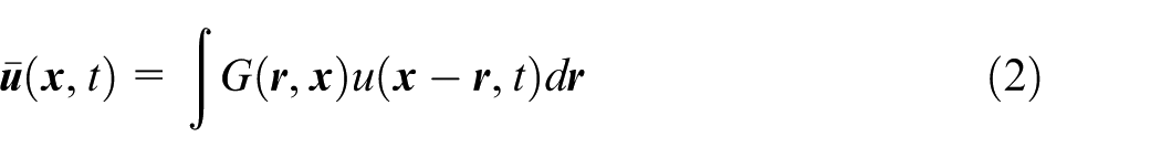
In LES, velocity

where
The subscripts
where
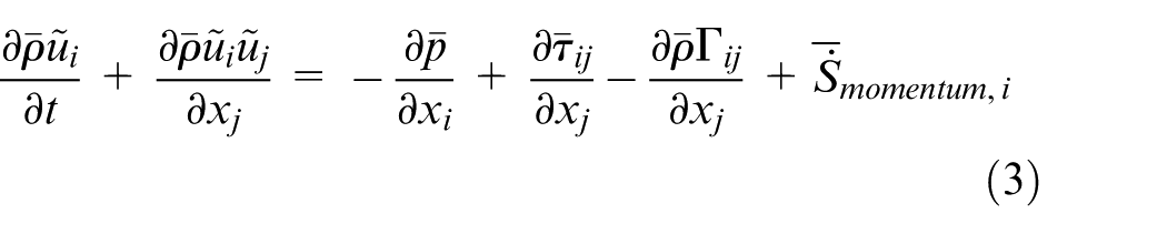
The momentum coupling between liquid and gas is represented by the source/sink term,
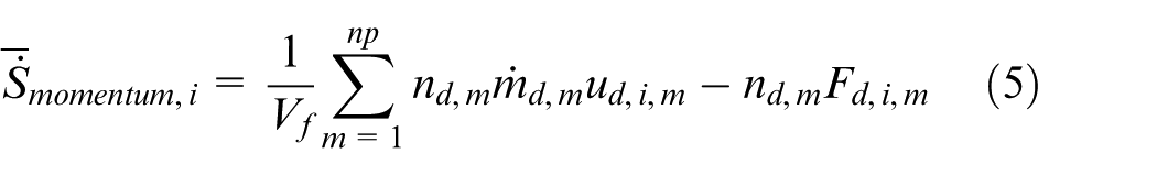
where
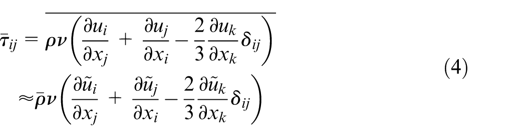
The

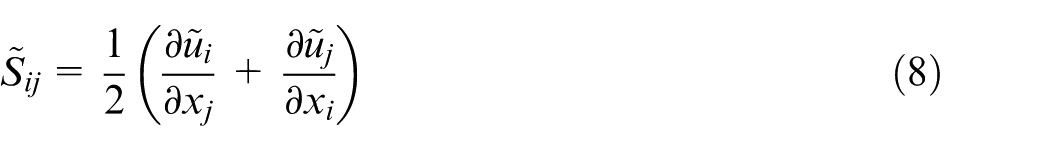
This study employs the dynamic structure sub-grid stress tensor model 29 with the addition of a near-nozzle viscosity model. This model has been well validated under conditions of high-speed gas jet and spray jet. 24 Prediction of fuel vapor penetration was greatly improved. It is given as
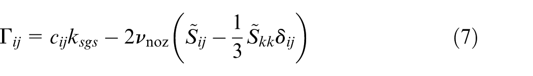
where
The first term on the right-hand side in equation (7) was developed by Pomraning and Rutland.
29
The form of the dynamic tensor coefficient
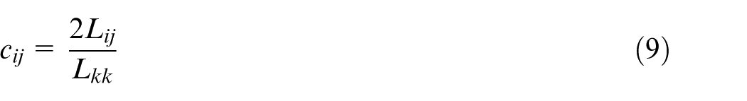
where

More features of this model can be referred to Rutland and colleagues.2,24,29,31 The sub-grid kinetic energy,
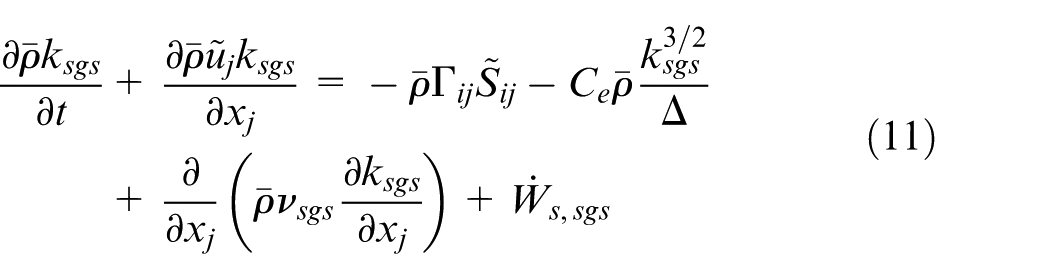
where
where the value of the constant,
Modeling of the SGS dispersion velocity,
The second term in equation (7) is an additional viscosity term added to the original dynamic structure model. 24 Unlike conventional viscosity-based models such as the Smagorinsky 32 model, the viscosity term here is only activated in the region where the strain rate is high. For sprays, the viscosity is only added in the near-nozzle region. The purpose of adding this term is to enhance sub-grid mixing in the near-nozzle region where a portion of energy-containing motions may not be adequately resolved under moderate grid resolution. This term is written as
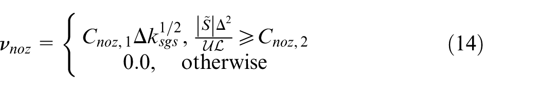
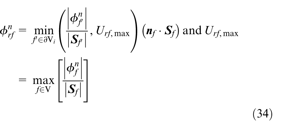
where
The model constant
Liquid-phase governing equations
The liquid phase is described by discrete Lagrangian parcels, with each parcel containing droplets having the same properties. Velocity of each parcel is updated by solving momentum equation for the drops
and the parcel position
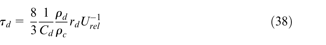
Mass and energy equations are described in Tsang and colleagues.24,28 The drag force on a droplet,
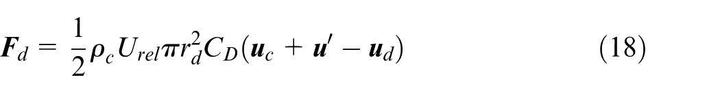
where

Note that the drag force calculation depends on the SGS dispersion velocity,

where the drag coefficient is
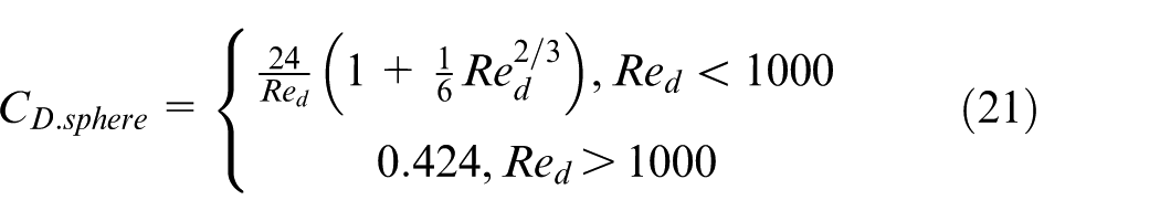
and the Reynolds number,
SGS dispersion model
The effect of sub-grid turbulent motions on spray dynamics are taken into account by the modeling of the SGS dispersion velocity,
It is assumed that the dispersion velocity can be decomposed into the deterministic and the stochastic parts

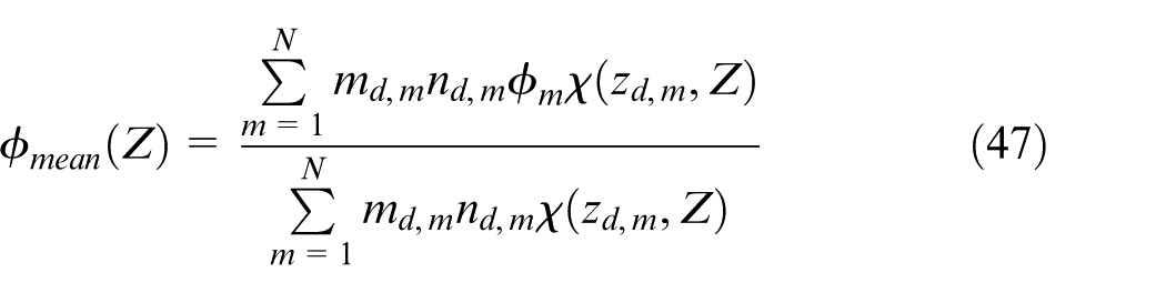
The deterministic part,
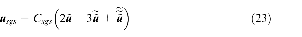
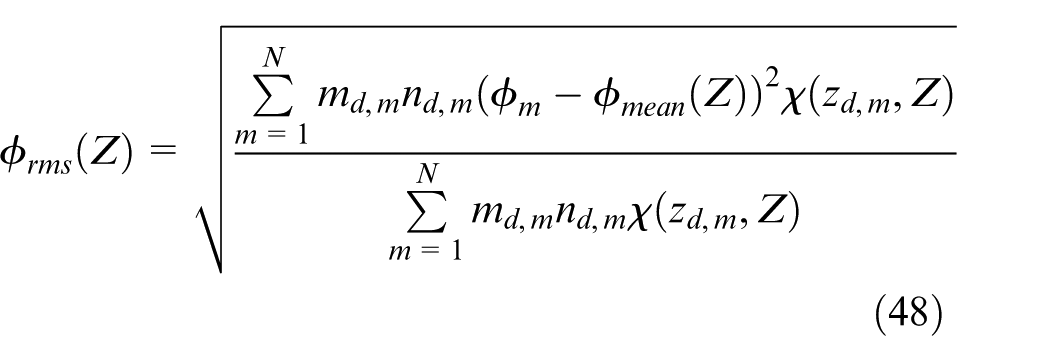
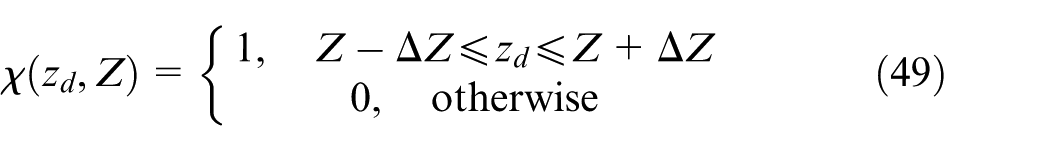
where
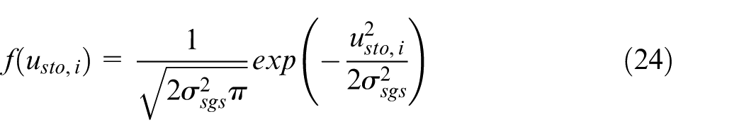
where the subscript i is denoted as the ith component of a vector, and the variance
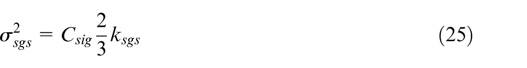
where
The SGS dispersion velocity of a parcel is sampled once every turbulence correlation time,
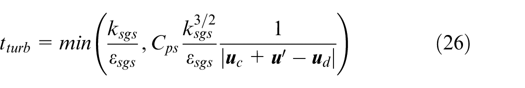
where
Another possible formulation of
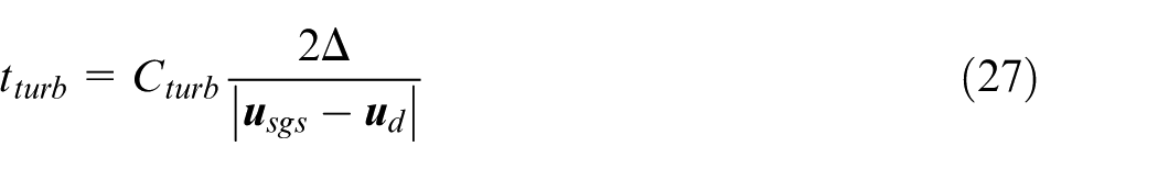
where
It is of interest to compare individual droplet trajectories predicted by equations (26) and (27). Figure 1 shows the trajectories of one liquid blob and its child droplets due to the KH breakup under the Engine Combustion Network (ECN) “Spray-A” conditions, as described in section “ECN Spray-A.” The trajectories predicted by equation (27) are apparently much more reasonable than those predicted by equation (26). We can see that in Figure 1(a), all the child droplet trajectories are straight lines. By examining the magnitude of
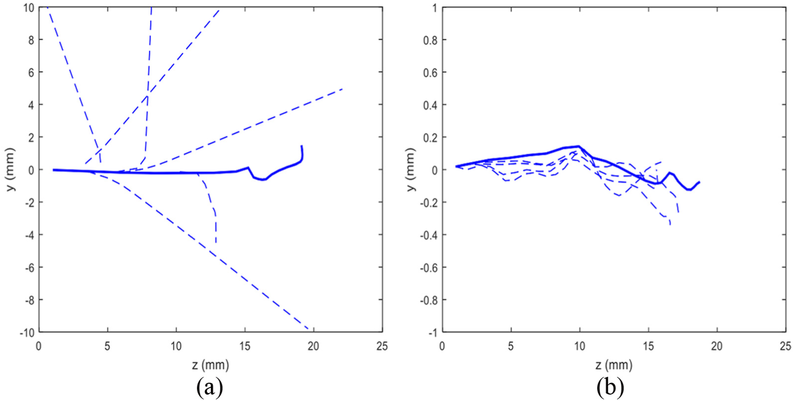
Trajectories of one of the liquid blobs and its child droplets due to the Kelvin–Helmholtz breakup predicted by (a) equation (26) and (b) equation (27) with
This comparison suggests that the simple modification from RANS-type spray models to LES may not work well without consideration of the different modeling methodologies between RANS and LES. For example, simple substitutions of RANS turbulent kinetic energy with LES sub-grid kinetic energy may not work well in all models. In the subsequent results, equation (27) is used to calculate the turbulence correlation time.
The effect of the variance of the Gaussian distribution and the turbulence correlation time on particle trajectories is studied in a simplified case before running full simulations. Consider a particle located at
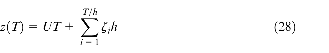
and
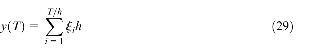
The y-position,
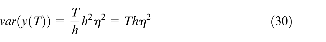
Hence, larger variance,

Particle sample paths calculated from equations (28) and (29) with different variances,
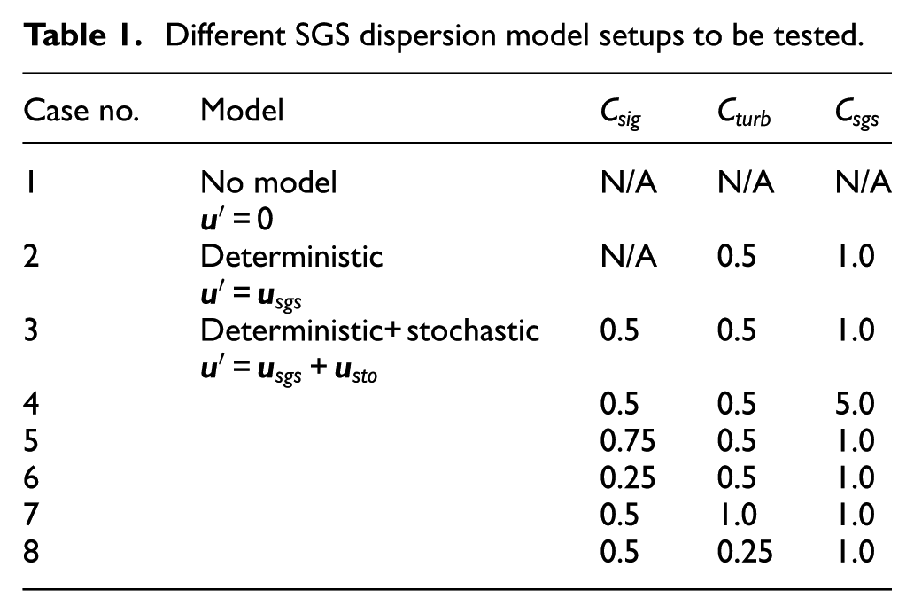
To investigate how different modeling methodologies of SGS dispersion impact the prediction of spray dynamics, simulations with different model setups as listed in Table 1 were run. Case 1 does not use any dispersion model. Namely, the dispersion velocity
Different SGS dispersion model setups to be tested.
VoF method
The VoF simulations reported in this article are performed with an algebraic solver, interFoam, which forms a part of a larger open-source distribution of computational mechanics solvers and C++ libraries of OpenFOAM®. 34 The solver is based on a finite volume discretization on collocated grids for the solution of two-phase incompressible flow. A thorough evaluation of solver performance with respect to a broad range of two-phase flows is reported in our previous publication. 35 The evaluation was based on the performance with respect to kinematics of advection, dynamics in inertia-dominated regime, and dynamics in the surface tension–dominated regime. An abbreviated description is provided here; a more detailed explanation can be found in Deshpande et al. 35
The first part of the solution consists of advancing the liquid fraction field,
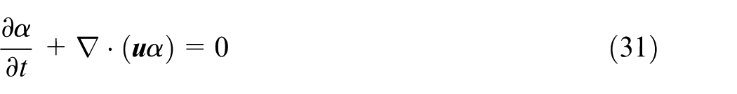
The liquid fraction represents the volume fraction of liquid occupying a given computational cell,
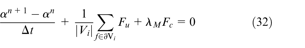
where the fluxes are defined as

here,
This compressive flux is used to mitigate the effects of numerical diffusion that would occur as a result of the sharp gradients in
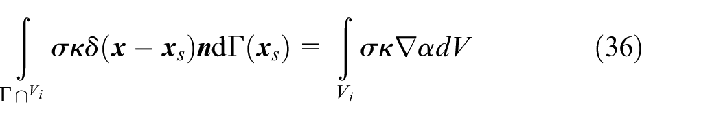
With respect to momentum, the following equation is solved
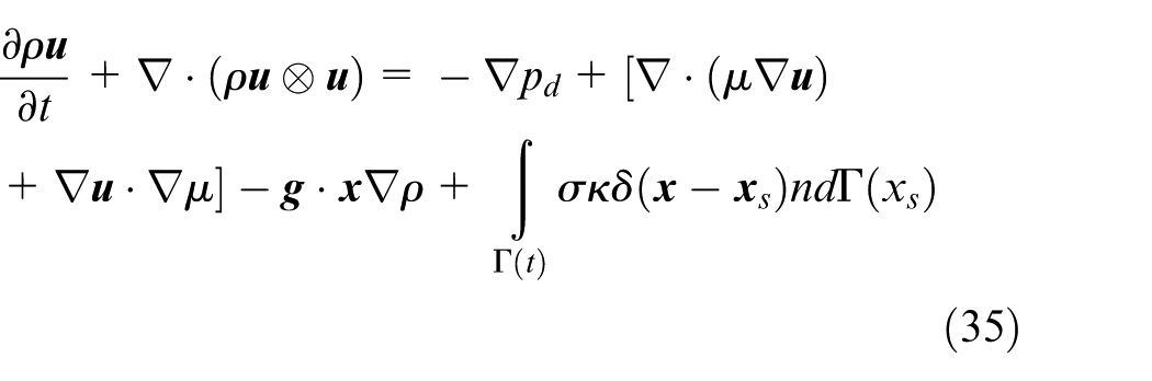
where the surface tension coefficient is given by
In the predictor step, the density and viscosity fields are regularized according to

The solution of the momentum equation is obtained via a Pressure-Implicit with Splitting of Operators (PISO) 38 iteration procedure. A predictor velocity is first constructed and then corrected to ensure momentum balance and mass continuity. Explicit formulation of the predictor velocity is a two-step process, where first the viscous, advective, and temporal terms in the momentum equation are used to generate a cell-centered vector field, which is then projected to cell faces using a second-order scheme. Contributions from surface tension and gravity terms are then added, concluding the predictor formulation. This procedure enforces a consistent discretization of surface tension and pressure gradient.35,39
Within the correction procedure, the pressure distribution is added to the flux of predictor velocity, and mass conservation is invoked to yield a Poisson equation for pressure. The linear system is then solved using a preconditioned conjugate gradient method, with diagonal incomplete Cholesky as the preconditioner. In this work, we have used three PISO steps to arrive at predictions for
Cases for validation
Two cases were selected to validate the LES models and to study the effects of the SGS dispersion. The first case is the VoF case with lower injection velocity. Under this condition, accuracy of the VoF calculation has been validated and grid convergence achieved. LES-predicted SGS dispersion velocities and VoF-derived SGS dispersion velocities were compared in this case, as discussed in section “Low injection velocity case.” Operating conditions of the second case, Engine Combustion Network Spray-A, are representative of typical Diesel engines. This case is used to validate key global quantities such as spray tip penetrations and fuel vapor spatial distribution. Detailed operating conditions are described in the following sections.
Low injection velocity case
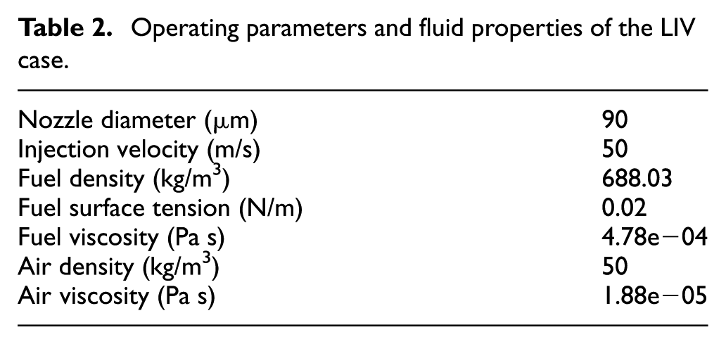
Operating parameters and fluid properties of the VoF case are summarized in Table 2. The fuel properties correspond to Iso-octane at 303 K and 4.5 MPa, and the air properties correspond to the same temperature and pressure. Vaporization is not considered in this case.
Operating parameters and fluid properties of the LIV case.
ECN Spray-A
The ECN database, 17 maintained by Sandia National Laboratories, is an online library collecting a large amount of well-documented spray experiments from different institutions for computational model validations. In this study, experiments done by Sandia National Laboratories and Argonne National Laboratory were used to validate the models. In the Sandia experiments, a single-hole injector is mounted in a constant-volume cube. In-chamber air temperature, pressure, and density are well controlled and are typical of Diesel engine operating conditions. The root-mean-square (RMS) velocity is approximately 0.7 m/s due to the fan inside the chamber, which is much smaller than the spray injection velocity (∼500 m/s).
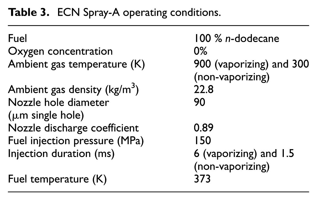
Several important quantities are measured by different experimental techniques.40–42 These include temporally resolved liquid and vapor penetrations and ensemble-averaged spatial fuel vapor distribution. The Advanced Photon Source facility at Argonne National Laboratory provides data in the near-nozzle region 43 and inside the nozzle. 44 Ensemble-averaged liquid projected mass density (PMD) is one of the valuable data used for validating the models in the near-nozzle region. The PMD data were obtained from X-ray radiography path-integrated measurements. The data provide a two-dimensional projection of liquid fuel mass onto a plane whose normal vector is orthogonal to the spray axis. In this study, the “Spray-A” experimental data were used to validate the models. The Spray-A operating conditions are listed in Table 3.
ECN Spray-A operating conditions.
LES and VoF computational setup
Physical models and numerical setup (mesh and numerical methods/schemes) are equally essential to have a successful spray simulation. The computational setup and comparison details between the LES and VoF methodologies are thus described in this section.
LES computational setup
A two-dimensional cut-plane of the three-dimensional domain and grid sizes are shown in Figure 3. Note that all cells are isotropic, namely,
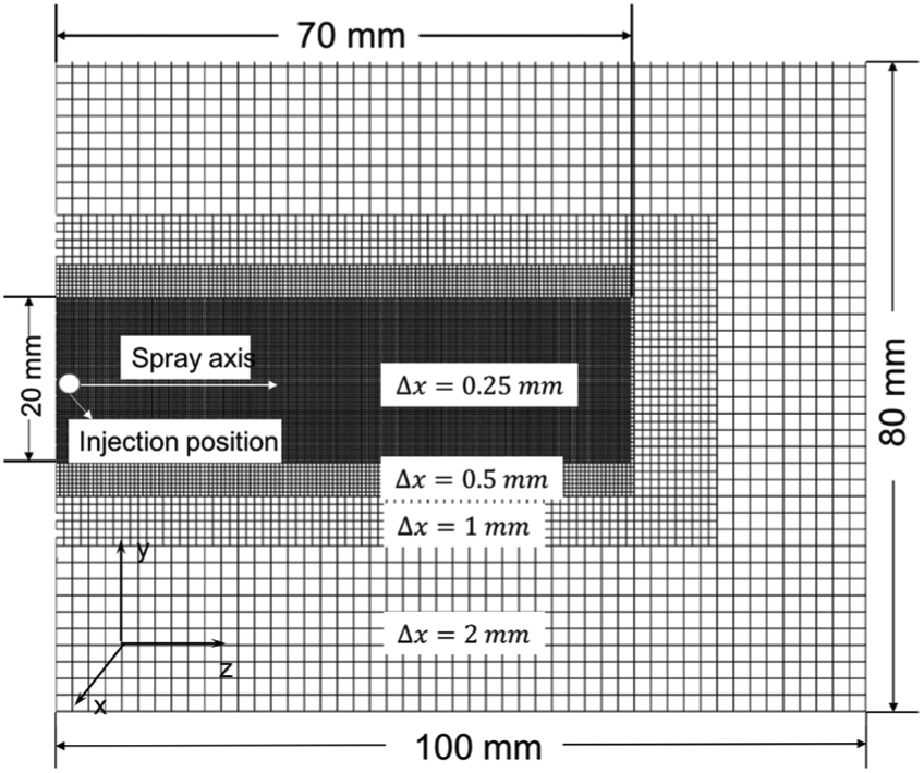
2D cut-plane of the LES computational mesh. This mesh was used in the both cases described in section “Cases for validation.”
In this study, the computational fluid dynamics (CFD) toolbox, OpenFOAM, 34 was used to solve the governing equations with the SGS and spray models implemented. The PISO pressure–velocity coupling algorithm 38 is used for solving the LES Navier–Stokes equations. OpenFOAM uses collocated grid system with a remedy similar to the Rhie–Chow scheme 45 for pressure/velocity oscillations. Euler implicit method is the time integration scheme for the gas-phase governing equations. The central cubic interpolation scheme is used for the convection term in the gas momentum equation. This combination was shown to be suitable for LES of free shear flows and sprays. 26 The computational time step size was fixed at 2.5e−07 s, resulting in maximum Courant number of ∼0.3 to ensure numerical stability.
The time step size,
The reason for this additional restriction is that the solution may become unstable due to the dramatic change of the dispersion velocity,
The stochastic Kelvin–Helmholtz/Rayleigh–Taylor (KH-RT) atomization and breakup model 28 is used. Model constants such as the KH time constant and the RT size constant are determined stochastically and dynamically according to local conditions. Compared to the original KH-RT model, 46 the stochastic model gave satisfactory simulation results in a wider range of operating conditions without tuning model constants. 28 Initial velocity of Lagrangian parcels is determined by the synthetic eddy method.28,47 This method simulates turbulence at nozzle outlet and generates time- and space-correlated injection velocity data without simulating flow inside the nozzle.
VoF computational setup
The VoF method is performed by the incompressible two-phase flow solver interFoam, as discussed in section “VoF method.” The computational domain along with the grid structure, which consists of hanging nodes, is shown in Figure 4. The domain extent is
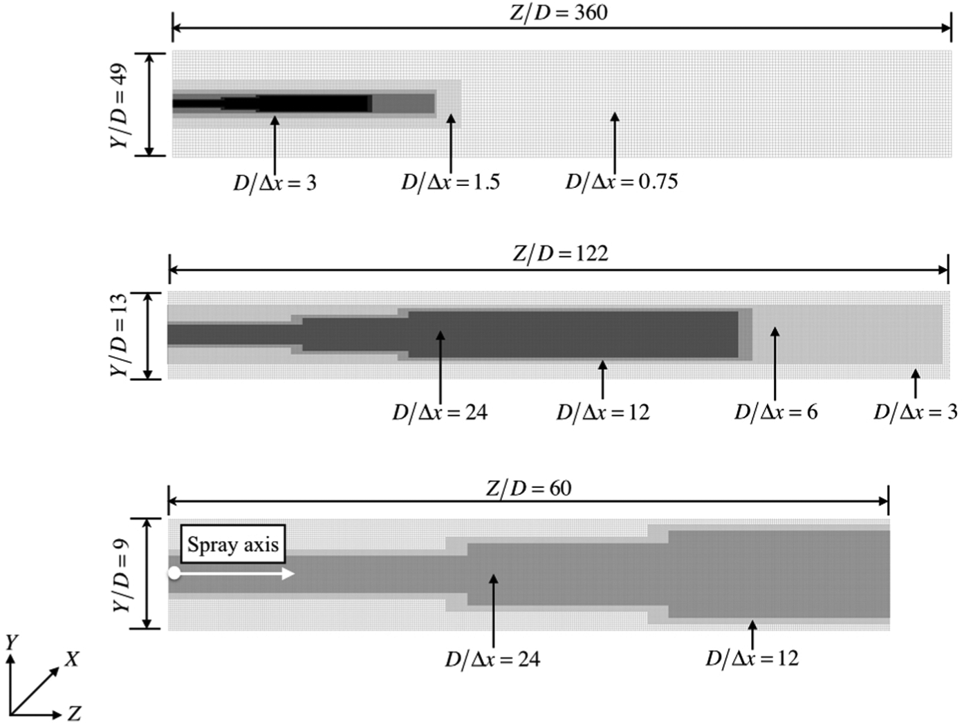
2D cut-plane of the VoF computational mesh; zoom-in view from top to bottom.
The identical physical setting used in LES is implemented in the VoF simulation. The fuel is iso-octane (
Method to compare LES and VoF data
In the low injection velocity (LIV) case, mean and RMS values of the SGS dispersion velocity modeled by LES and computed directly from VoF were compared. This section introduces how to obtain SGS dispersion velocity from VoF solutions and how to perform averaging in VoF and LES to obtain mean and RMS values.
Data processing in VoF
Computational volumes (shown in Figure 5) are employed to volume average the VoF data for use in LES. These volumes are of the same size as the LES mesh
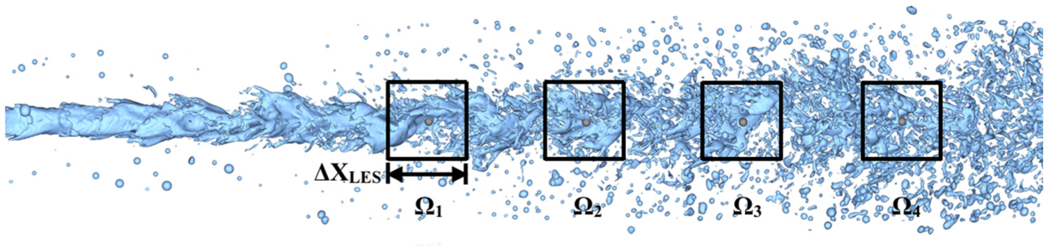
Computational volumes (
The gas velocity,
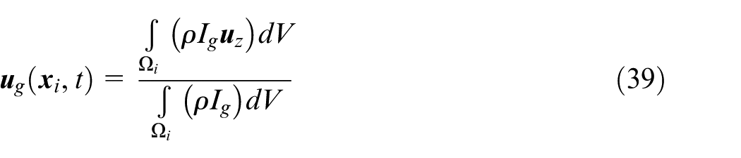
where
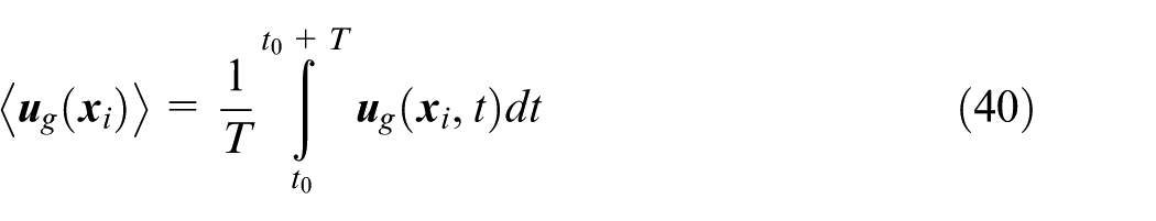

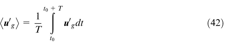
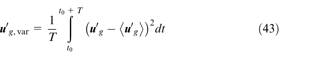
The beginning of the time integration is set
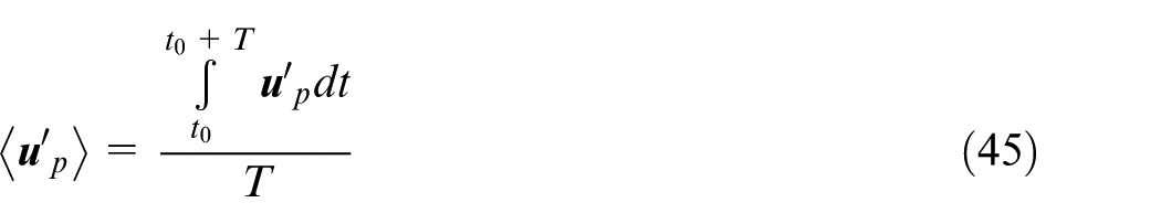
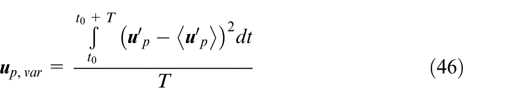
Data processing in LES
The parcel-based dispersion velocity,
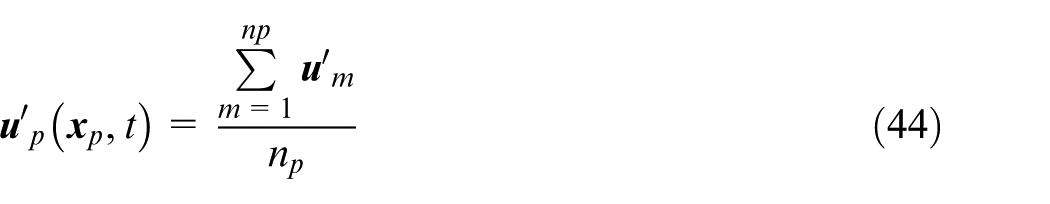
where
and
where
Results and discussion
This section presents results from the two test cases described in section “Cases for Validation.” For the LIV case, SGS dispersion velocities modeled by LES and calculated by VoF are compared. For the ECN spray cases, LES-predicted liquid PMD and liquid and vapor penetrations are compared to the available experimental data. Also, the effects of the SGS dispersion on liquid and gas motions are discussed.
LIV case
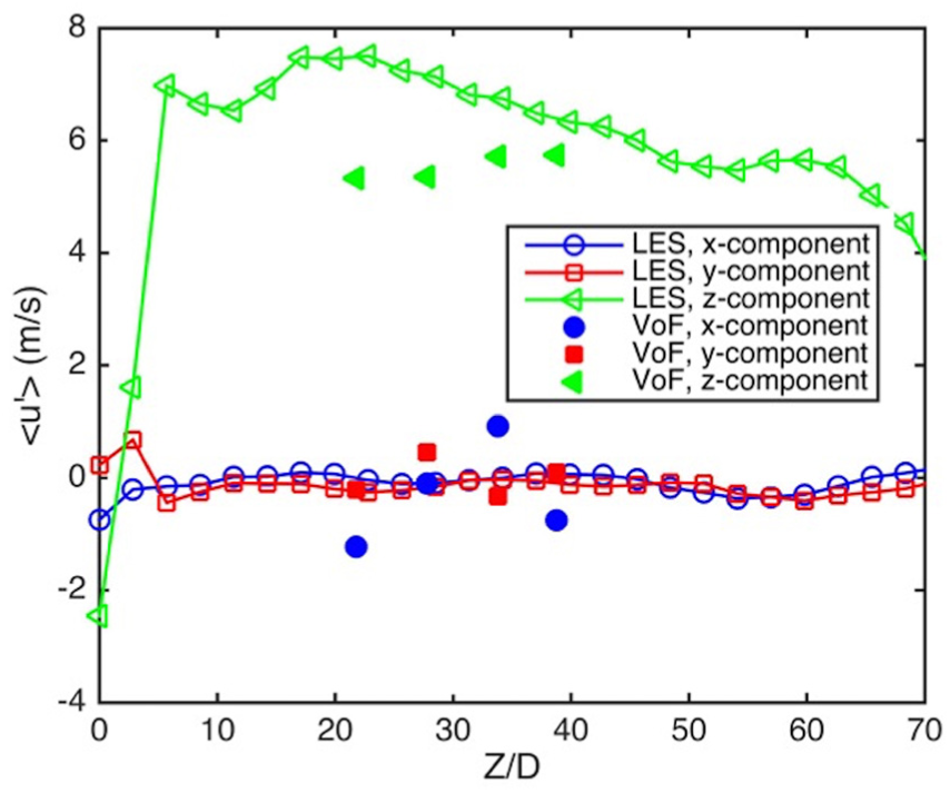
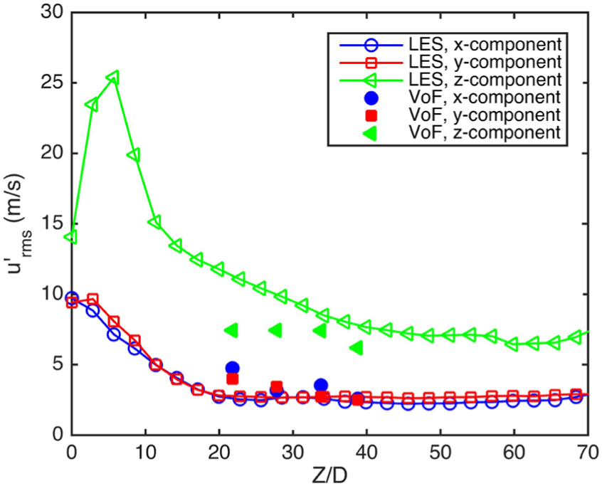
Figures 6 and 7 show the comparison of the three components of the mean and RMS dispersion velocities at Y/D = 0 calculated by VoF (equations (42) and (43)) and predicted by LES (equations (45) and (46)) Case 3. The comparison of the LES Case 4 results and the VoF results at Y/D = 0 and Y/D = 1 are shown in Figures 8–11. The VoF data have been shifted to the left by 20 nozzle diameters for comparison. This is to compare LES and VoF data in the same breakup regime where breakup of liquid core and dramatic increase in gas–liquid interface area occur. In the VoF calculations,20,48 this occurs in the region between the upstream initial instability development and downstream dispersed droplets. In LES, this region is modeled by the concept of the breakup length in the stochastic KH-RT model. Within the breakup length, only the primary KH breakup can occur; beyond the breakup length, both KH and the secondary RT breakup which tends to produce smaller drops can occur. It was found that the VoF calculation predicted longer liquid core, and thus, the breakup of liquid core and dramatic increase in gas–liquid interface area occurred further downstream than LES by 20 nozzle diameters. This may be due to the different boundary conditions between VoF and LES. The VoF simulation used a top-hat uniform velocity profile, while the LES simulation employed the blob injection with the synthetic eddy perturbation.
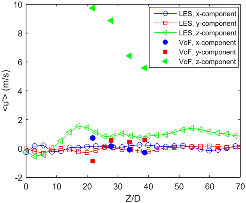
Mean values of the SGS dispersion velocities atY/D = 0. The LES results are from Case 3
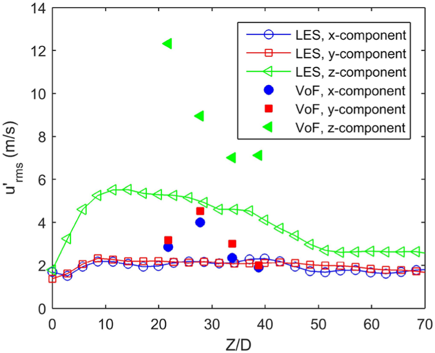
RMS values of the SGS dispersion velocities atY/D = 0. The LES results are from Case 3
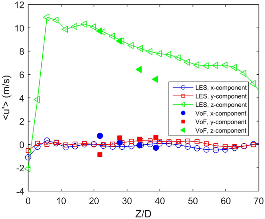
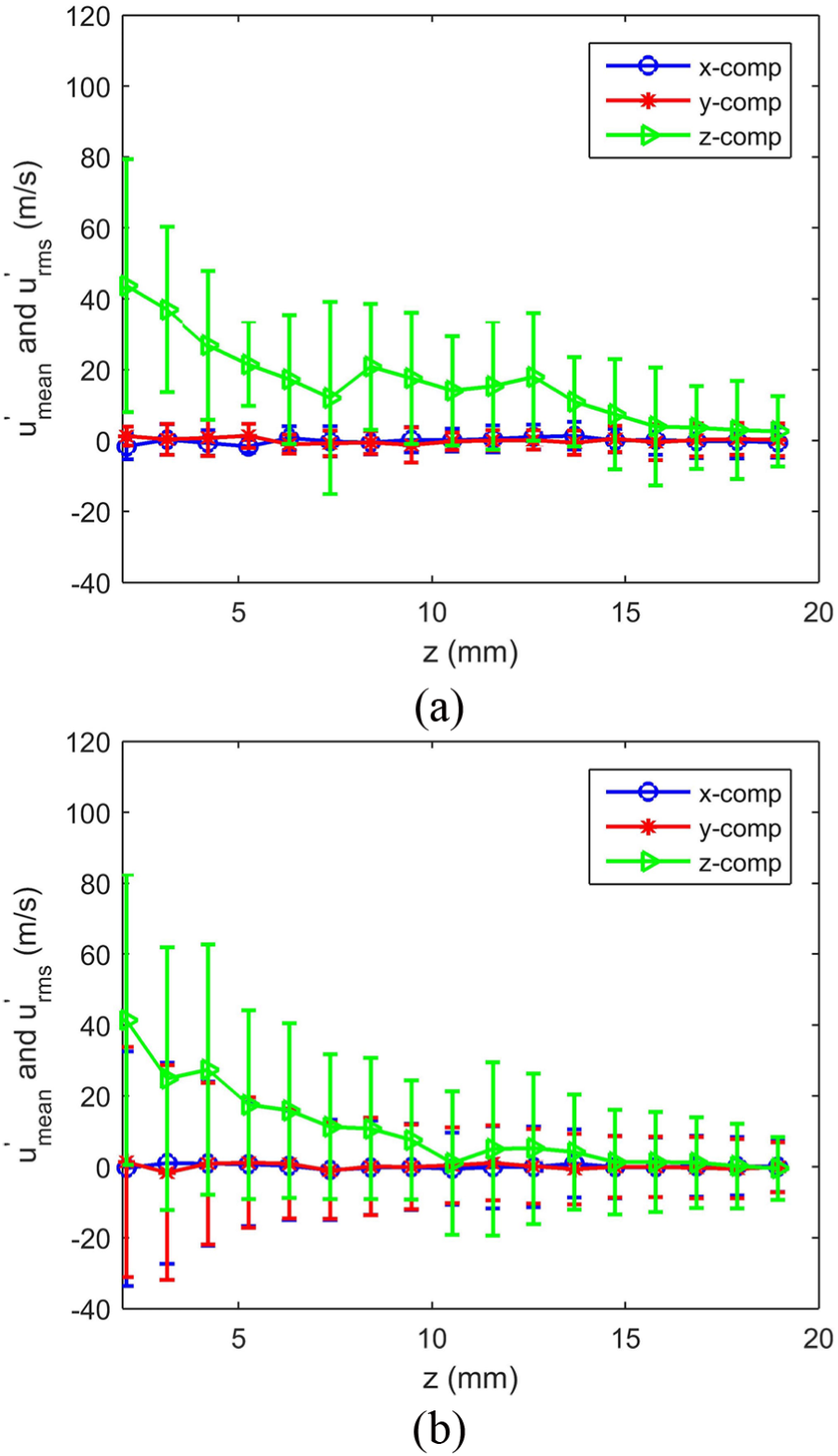
Mean values of the SGS dispersion velocities atY/D = 0. The LES results are from Case 4
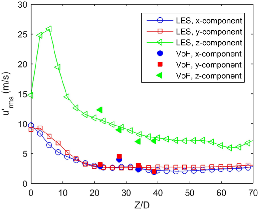
RMS values of the SGS dispersion velocities at Y/D = 0. The LES results are from Case 4
Mean values of the SGS dispersion velocities atY/D = 1. The LES results are from Case 4
RMS values of the SGS dispersion velocities atY/D = 1. The LES results are from Case 4
Several observations from the VoF data are discussed as follows. The mean values in the x- and y-directions are close to zero at the spray axis due to the axisymmetric jet, which is expected, but the axial component is greater than zero. At the off-axis locations (Y/D = 1), the x and the y components of the mean dispersion velocities are also close to zero predicted by VoF and LES as shown in Figure 10. The Y/D = 1 location may be still close to the centerline at axial locations greater than Z/D = 20. Statistics at further off-axis locations were not computed due to the restricted region of grid refinement in the VoF calculation. The RMS values in the two lateral directions are not zero at the spray axis and off the spray axis (Y/D = 1) and are smaller than the RMS values in the axial direction. Note that the x and y components of the RMS values computed in VoF were not exactly matched. The difference stem from the fact that in the near field, the momentum interaction between phases is quite a bit more complicated than an interaction described by a populations of spherical elements as captured in the LES Lagrangian–Eulerian simulations. This complexity is the result of the dynamic shape of the interface in this region of the domain, which unavoidably affects the resulting turbulence and is reflected in different components for the SGS dispersion velocities. The VoF results revealed that the SGS dispersion velocity is anisotropic at and near the spray axis. The current model is able to capture the anisotropy. Note that the anisotropy must result from the deterministic part of the model (equation (23)) since the stochastic part (equation (24)) is assumed to be isotropic. However, Case 3
Note that the VoF results are dependent on the choice of the volume size and shape for the averaging operation (equation (39)). In this study, the volume is assumed to be equal to the LES cell volume. In the present implicit LES approach, discretization of derivatives acts as a low-pass filter, but the size and the shape of the filter volume are not explicitly defined. Thus, computational cell volume in LES being equal to the LES filter volume is indeed an assumption. This assumption is used in calculating model terms in which filter length scales are required, such as the SGS viscosity (equation (12)). Since there may be a reasonable range of volume sizes for the averaging operation in VoF, this study is more focused on qualitative comparison rather than tuning the dispersion model constants to perfectly match the current VoF data. For Case 4, qualitative features of the SGS dispersion can be well captured. These include anisotropy and x and y components of the RMS values being smaller than the z-component of the RMS values. Also, the LES and VoF results are in the same order of magnitude. In the next section, the role of the SGS dispersion model in practical Diesel spray simulations is investigated.
ECN Spray-A cases
Non-vaporizing and vaporizing ECN spray results are discussed in this section.
Non-vaporizing sprays
Simulated spatial distributions of liquid mass are compared against the X-ray ECN data as shown in Figures 12 and 13. The experimental results were time- and ensemble-averaged. Simulation results were time-averaged and spatial-averaged in the azimuthal direction which is the statistically homogeneous direction. The duration of the time averaging, 0.4–1.2 ms, is the same in the simulations and in the experiments. As shown in Figures 12 and 13, the liquid spray width is ∼0.8 mm at z = 5 mm and ∼2 mm at z = 10 mm. As shown in Figure 1(a), however, the child droplets can reach as far as 10 mm in the lateral direction. This is an overprediction. This comparison shows that the RANS turbulence correlation time model (equation (26)) predicts the existence of spray droplets at the outer region of the spray where no droplets were detected by experimental measurements. Again, this confirms the unreasonable droplet trajectories predicted by the RANS model.
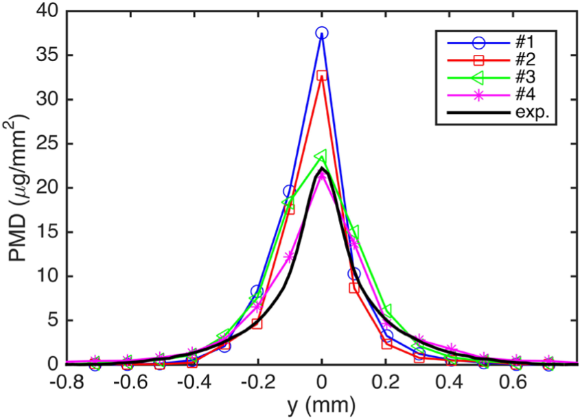
Lateral PMD profiles at z = 5 mm. Case 1:
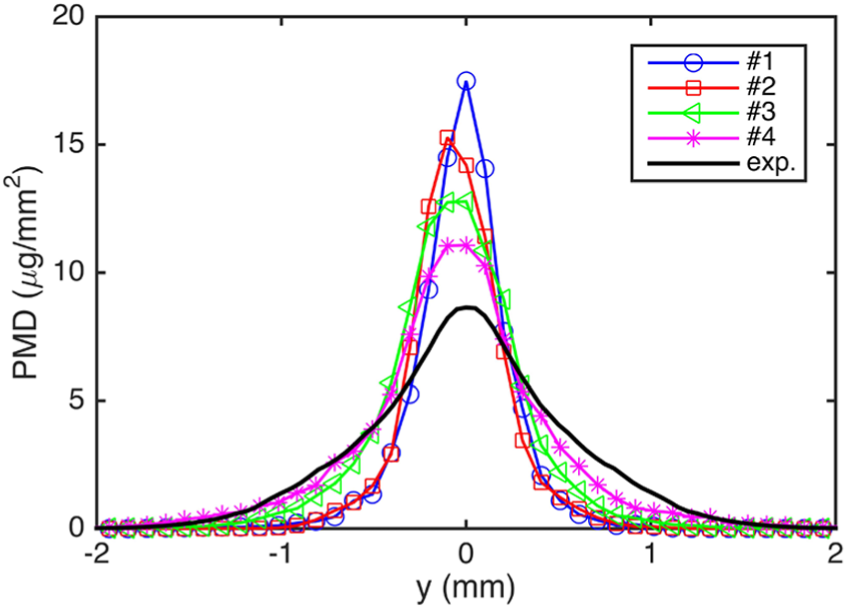
Lateral PMD profiles at z = 10 mm. Case 1:
The SGS dispersion model has impact on the prediction of liquid spray width as shown in Figures 12 and 13. Without using the stochastic dispersion model (Cases 1 and 2), the PMDs at y = 0 are significantly overpredicted, and the spray width is underpredicted in the downstream region (z = 10 mm). The stochastic model (Cases 3 and 4), however, predicts wider spray and improves the prediction at y = 0. These differences can be explained by Figure 14, showing the mass-weighted and spatially averaged mean and RMS values of the dispersion velocity at different axial locations at 0.6 ms. Mass-weighted and spatially averaged mean and RMS values of any properties of Lagrangian parcels,
and
where
where
Mass-weighted and spatially averaged dispersion velocities predicted by (a) Case 2
Figure 15 shows the qualitative comparison of the instantaneous PMD contours predicted by the different values of
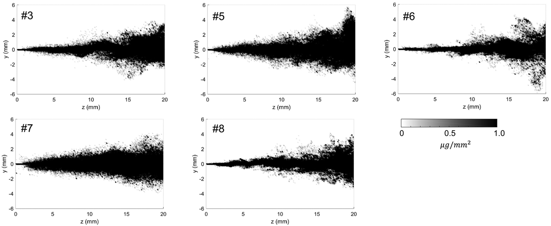
Instantaneous PMD contours at 0.55 ms predicted by the different values of the model constants,
Figures 16 and 17 show the quantitative comparison of the PMD profiles predicted by the different values of
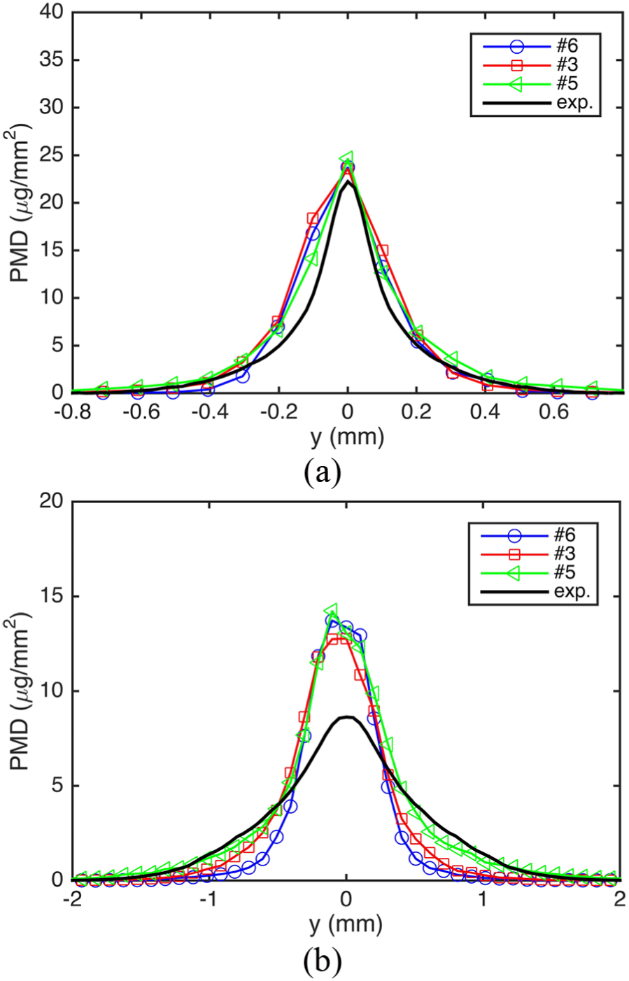
PMD profiles at (a) z = 5 mm and (b) z = 10 mm predicted by the different values of the SGS dispersion model constant,
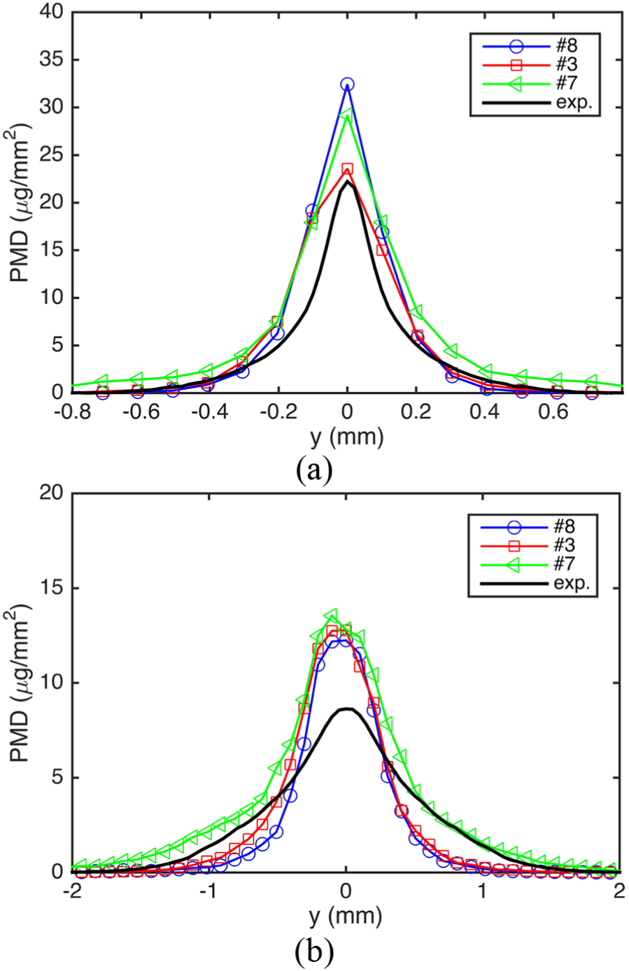
PMD profiles at (a) z = 5 mm and (b) z = 10 mm predicted by the different values of the SGS dispersion model constant,
The results above show that SGS dispersion has a profound effect on the spatial distribution of liquid mass. Here, the effect of the SGS dispersion model on gas-phase solutions are examined. Qualitative comparison is made first by visualizing vortex structures by plotting iso-surfaces of the Q-criterion. The Q-criterion
49
is defined as
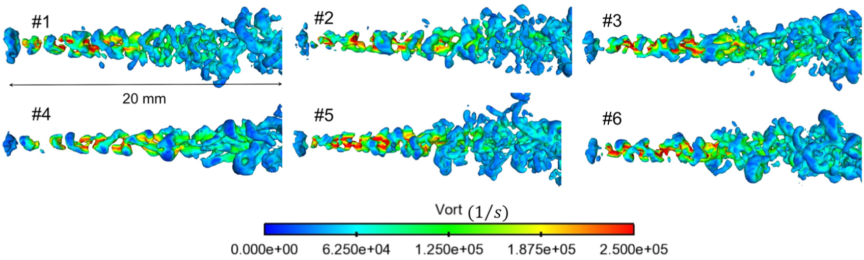
Q-criterion iso-surfaces at 0.4 ms,
Quantitative comparisons are made by plotting mean and RMS streamwise gas velocity radial profiles at three different axial locations, as shown in Figures 19 and 20. Time averaging from 0.4 to 1.2 ms and spatial averaging in the azimuthal direction were performed to obtain the mean and RMS values. There are some noticeable differences of the mean and RMS values predicted by the different model setups at the centerline and at z = 5 and 15 mm. At z = 5 mm, the RMS value at centerline predicted by Case 4 is lower than those predicted by the other cases. This might correspond to less small-scale structures predicted by Case 4 as shown in Figure 18. Nevertheless, the overall shapes of the profiles predicted by the different model setups are close to each other. At 25 mm, these profiles are almost on top of each other. Again, compared to the sub-grid stress model which has profound impacts on the prediction of gas entrainment as shown in the previous studies, these results suggest that the SGS dispersion model plays a less critical role in predicting air entrainment under Diesel spray conditions.
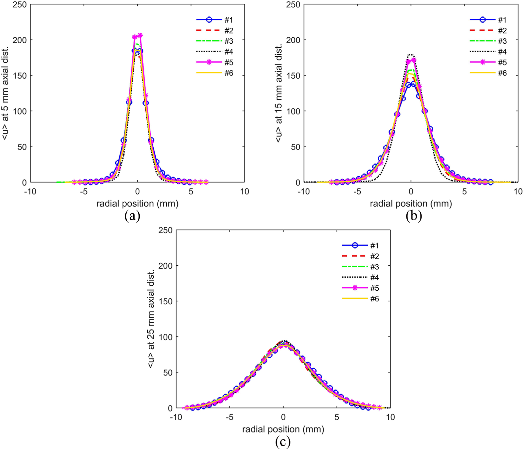
Mean streamwise gas velocity profiles predicted by the different SGS dispersion model setups at three axial locations: (a) 5 mm, (b) 15 mm, and (c) 25 mm. Case 1:
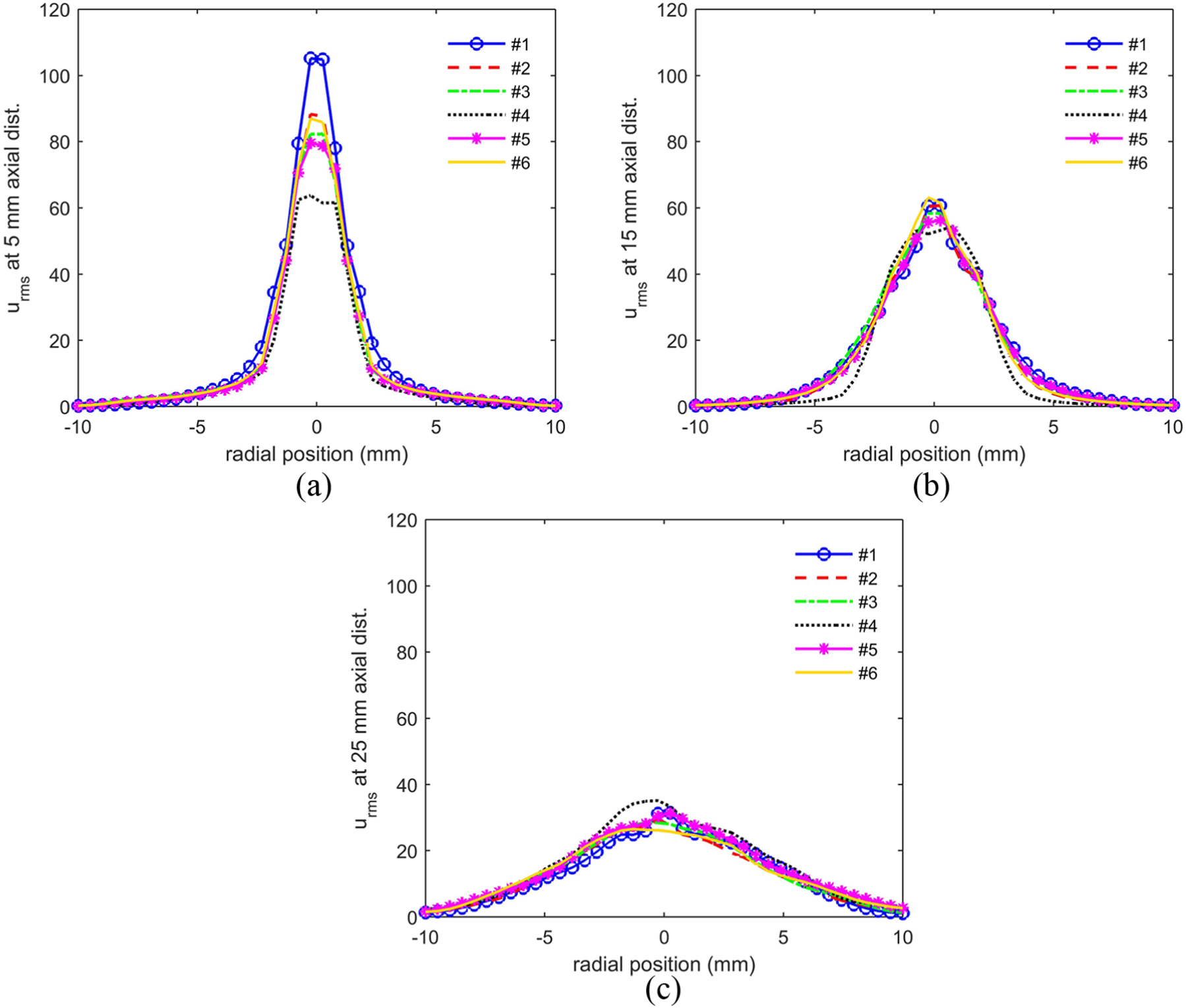
RMS streamwise gas velocity profiles predicted by the different SGS dispersion model setups at three axial locations:(a) 5 mm, (b) 15 mm, and (c) 25 mm. Case 1:
The fact of the SGS dispersion model being less important in predicting gas-phase quantities is further examined. Figure 21 shows the time series of the convection, sub-grid stress, pressure gradient, and spray momentum source terms in the gas-phase z-momentum equation, predicted by Case 6 at different positions. The drag force term predicted by Cases 4, 5, and 6 are quite close to each other, meaning that the momentum budget predictions should also be similar. Hence, Case 6 should be sufficiently representative for the momentum budget analysis. In the upstream region, 5 mm from the injector, the magnitude of the spray momentum source term is comparable to the convection term, meaning a significant amount of momentum transfer from liquid to gas. Figure 22 also shows a sharp decrease in the drag force within 5 mm. Moving further downstream to 10 and 15 mm from the injector, the magnitude of the spray momentum source term is much smaller than the convection, sub-grid stress, and pressure gradient terms, and it is negligible at 15 mm. This corresponds to the small drag force downstream as shown in Figure 22. Thus, air entrainment and subsequent gas jet development due to spray injection is mainly initiated in the near-nozzle region (within ∼5 mm). In this region, liquid injected from the nozzle carry significant amount of momentum and experience little deceleration as shown in Figure 24. Figure 23 shows that within 5 mm, the dispersion ratio,
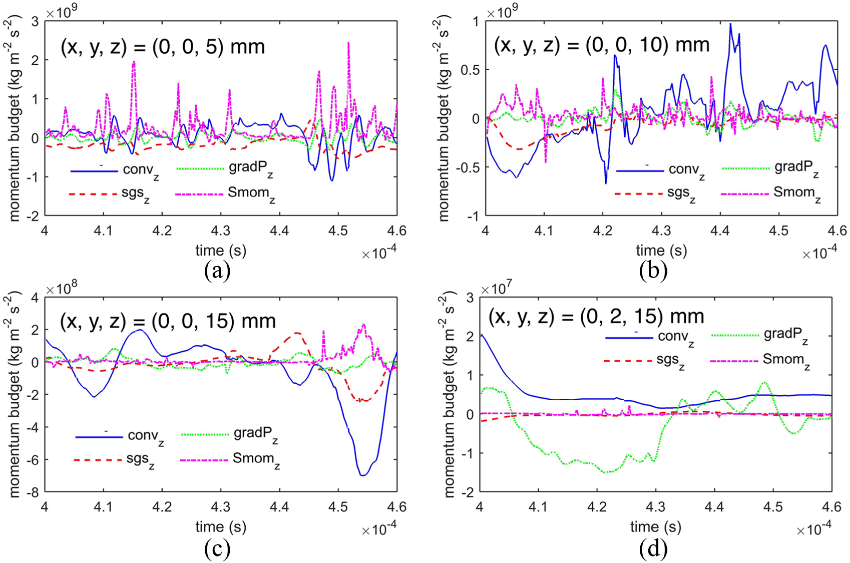
Time series of the z-momentum budgets at (a)
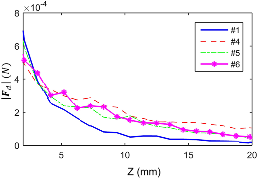
Mass-weighted and spatially averaged drag force magnitude versus distance from the injector predicted by Case 1
Mass-weighted and spatially averaged dispersion ratio versus distance from the injector predicted by Case 4
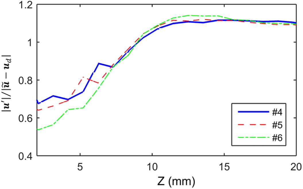
In the downstream region (z > 10 mm), the dispersion velocity magnitude is comparable to the resolved slip velocity as shown in Figure 23, indicating that the dispersion model is more important in determining the droplet motion. Figure 24 shows that the larger the dispersion velocity magnitude, the larger the acceleration magnitude. This is also consistent with Figures 13 and 16(b) indicating that larger dispersion velocity results in more diffusion of droplets. Another note is that in the 15 mm downstream region, a quasi-equilibrium has been established between the two phases. This is evidenced by large acceleration of droplets (Figure 24) equivalent to short response time to ambient flows and negligible drag force term in the gas momentum equation (Figure 21(c) and (d)) indicating that slip velocity approaches zero.
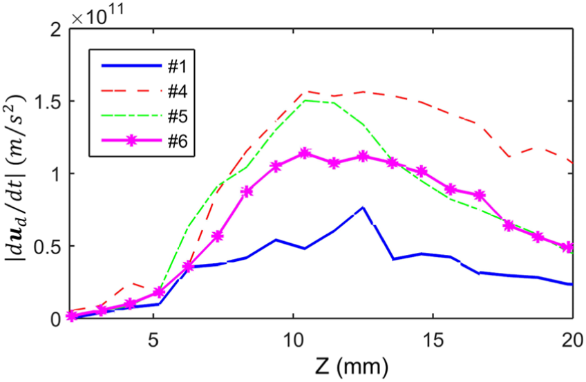
Mass-weighted and spatially averaged droplet accelerations versus distance from the injector predicted by Case 1
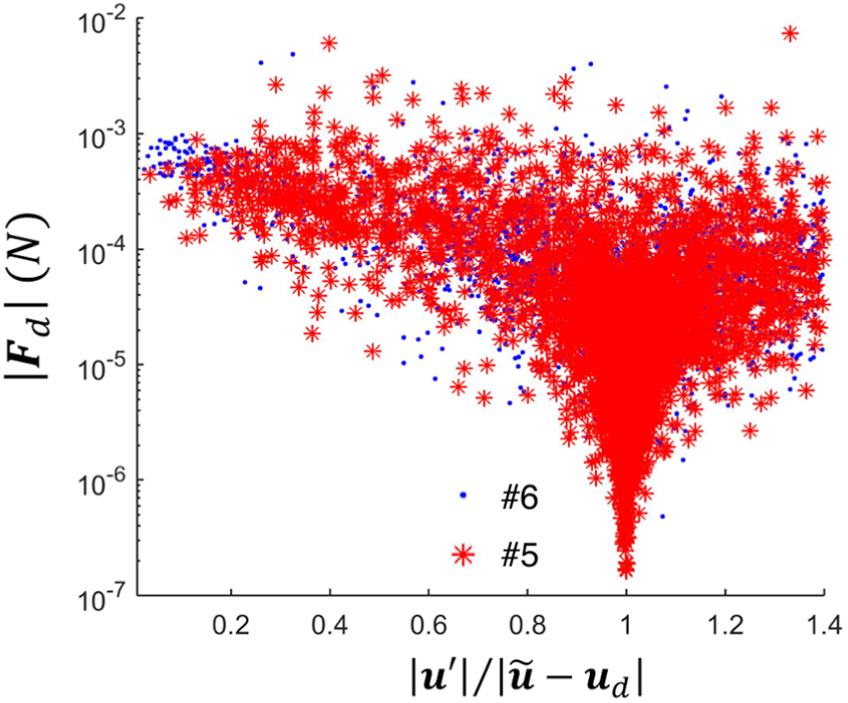
The main point from Figures 21–24 is that the SGS dispersion model does not have significant effect on the air entrainment process, but has significant impact on the droplet motion and droplet spatial distribution downstream of the spray where the momentum transfer from liquid to gas is small. In fact, a correlation between the dispersion ratio,
Drag-dispersion ratio scatter plot predicted by Case 6
Additional note is on the singularity at a dispersion ratio of 1 in Figure 25. This occurs where droplets are at periphery of the spray where the resolved gas velocity,
Vaporizing sprays
Simulation results of the vaporizing Spray-A are compared against the available experimental data. As shown in Figure 26, larger
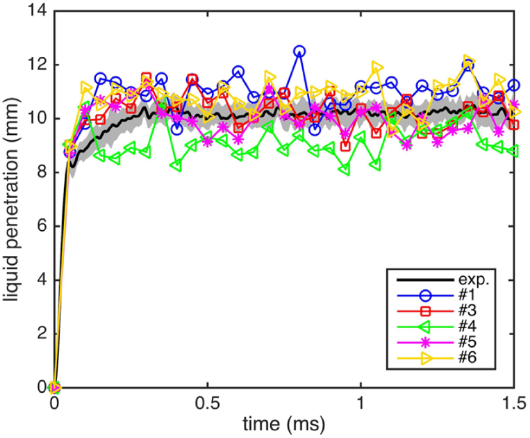
Liquid penetrations predicted by Case 1
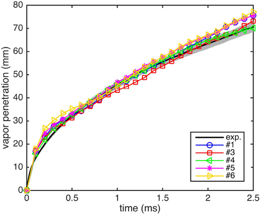
Vapor penetrations predicted by Case 1
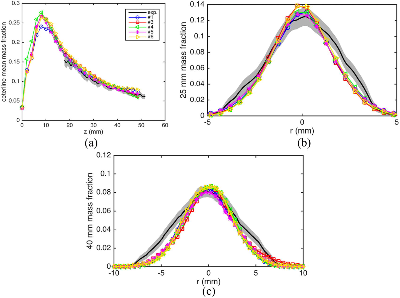
Mean fuel vapor mass fraction profiles at (a) centerline, (b) 25 mm, and (c) 40 mm axial distances predicted by Case 1
Summary and conclusion
This work is focused on the development and evaluation of the SGS dispersion model used in LES of engine sprays. The model computes the dispersion velocity term needed in the calculation of the slip velocity used in a number of spray models. It is assumed that the dispersion velocity is decomposed into a deterministic part and a stochastic part. The deterministic part is calculated by the approximate deconvolution method, which recovers the largest unresolved scales from the solution of the filtered velocity. Small-scale sub-grid motions are taken account by the stochastic part of the model. The stochastic part of the dispersion velocity is assumed to be isotropic and Gaussian distributed. The dispersion velocity is sampled once every turbulence correlation time, the time needed for a droplet to traverse an eddy in SGSs. A new form of the turbulence correlation time for LES was proposed to replace the RANS turbulence correlation time, which was shown to predict unreasonable droplet trajectories.
Mean and variance values of the SGS dispersion velocity were directly computed from the solutions of the high-fidelity VoF simulations. The injection velocity for the VoF case is approximately 1/10 of typical Diesel injection velocity. The data were compared to LES results. The VoF data revealed that both mean and variance of the SGS dispersion velocity are not isotropic, with magnitudes in the streamwise direction larger than those in the other two lateral directions. The anisotropic feature is well captured by the SGS dispersion model. The VoF and LES Case 4 results showed a good match.
Effects of SGS dispersion on Diesel spray conditions were studied using ECN data. It was found that neglecting the SGS dispersion resulted in the poor predictions of the spatial distribution of liquid mass. The stochastic part of the SGS dispersion model enhanced the diffusion of droplets and improved the prediction. In particular, larger values of the constants
It is suggested that one cannot neglect the SGS dispersion model in LES of Diesel engine sprays since it provides more reasonable prediction of the spatial distribution of liquid mass, although the model plays a less important role in predicting gas entrainment due to high-speed spray injection. One direction of future research is to examine whether the same conclusion is still applied to gasoline sprays.
Footnotes
Acknowledgements
The authors acknowledge additional support from CEI, Inc. through their EnSight software.
Declaration of conflicting interests
The author(s) declared no potential conflicts of interest with respect to the research, authorship, and/or publication of this article.
Funding
The author(s) disclosed receipt of the following financial support for the research, authorship, and/or publication of this article: This work was supported by Caterpillar Inc.