
Abstract
A review of using large-eddy simulation (LES) in computational fluid dynamic studies of internal combustion engines is presented. Background material on turbulence modelling, LES approaches, specifically for engines, and the expectations of LES results are discussed. The major modelling approaches for turbulence, combustion, scalars, and liquid sprays are discussed. In each of these areas, a taxonomy is presented for the various types of models appropriate for engines. Advantages, disadvantages, and examples of use in the literature are described for the various types of models. Several recent examples of engine studies using LES are discussed. Recommendations and future prospects are included.
1 Introduction
It is generally agreed that the next generation of turbulence modelling in computational fluid dynamics (CFD) for many applications will be some form of large-eddy simulation (LES). For the appropriate applications, LES can offer significant advantages over traditional Reynolds Averaged Navier Stokes (RANS) modelling approaches. For example, in internal combustion (IC) reciprocating engines, LES can be used to study cycle-to-cycle variability, provide more design sensitivity for investigating both geometrical and operational changes, and produce more detailed and accurate results. There are also characteristics of IC engines, such as inherent unsteadiness and a moderately sized domain, that are well suited to LES. This is not to say that LES will replace RANS. There are pluses and minuses for both methods and users should pick the appropriate tool for the topics being studied. However, as inexpensive computing power increases, the ability to use LES in IC engine simulations is increasing.
As LES gains in capability, there is the potential for a larger set of people using the models and a broader application of LES to engines. In addition, LES in IC engines is new, and there are potential uncertainties and ambiguities since a generally accepted ‘best practice’ is still developing. This motivates the objective of this paper, which is to describe and categorize the current LES models that could have application to engines and to evaluate their suitability and potential predictive capability for use in engine CFD. This is meant to help users of engine CFD be better informed about LES so that it can be used wisely.
In several important ways, IC engines are a good application for LES. The flow physics are well suited to LES in that: (a) the flows are inherently unsteady due to moving piston and valves, (b) large-scale flow structures are usually important, (c) the Reynolds numbers of engine flows are modest, commonly of the order of 10 000 to 30 000, and (d) the domain of interest is primarily confined and moderate in size. The last two points result in grid requirements that are more limited than other applications such as aeronautical flows. This has even tempted some researchers to claim that they are approaching direct numerical simulation (DNS) engine simulations [1], although this is probably overstating the situation. In addition, the low Reynolds numbers in engines and the reduced, or even missing, inertial range indicate that traditional LES models may not work as well in these applications.
In contrast, the complex physical processes that occur in engines increase the difficulty for any CFD modelling, including LES. Models (sometimes called submodels) are required, not only for turbulence, but also for liquid sprays, combustion, and various scalar processes. This means that LES modelling for engines should be more than just using a turbulence model, such as the dynamic Smagorinsky model, and leaving all of the other submodels the same as RANS models. Unfortunately, this approach is fairly common, as shown in a later section, and is another motivation for this report. Proper use of LES in engines requires potential modification of many submodels to make them consistent within the LES context.
The evaluation of LES models in this review is focused on IC engine cylinder flows, including the gas exchange, spray, and combustion processes. This is because of their primary importance in determining engine fuel efficiency and emissions. The review contains three major sections. First, a general discussion of LES is provided. This includes specific IC engine issues and uses RANS to provide a context for understanding LES. Second, the various types of LES models that might be applied to engine simulations are listed and categorized. This includes lists and discussions for basic turbulence models, combustion models, scalar mixing models, and fuel-spray models. Next, there is a section that presents several recent studies that use LES to simulate IC engines. This section uses the model taxonomy from the previous section to help categorize the types of LES models being used in the various studies. The review concludes with a section that discusses future prospects of LES of engines.
In this article, it is assumed that the reader is familiar with basic turbulence modelling in engine CFD applications and has some familiarity with the concepts underlying the LES approach. While some background information is provided, the emphasis in this paper is on describing and evaluating current LES approaches as they pertain to IC engines. The report does not include a tutorial on LES modelling or detailed descriptive equations of the models discussed. Some details are provided in the Appendices, but readers seeking detailed model descriptions or a basic primer on LES are encouraged to consult excellent resources of general LES theory and modelling presented by Ferziger [2], Fureby et al. [3, 4], Geurts [5], Piomelli [6], and Pope [7]. While there are interesting advanced LES models in the literature, they are not addressed here since the focus is on approaches that are mature enough to show promise for near-term successful use in real engine simulations.
2 General LES Background
The word ‘LES’ is becoming very common as a way to describe a variety of turbulent flow simulations. Some researchers working on CFD turbulence models may describe their models as LES, even if they may not follow traditional approaches. Generally, most people use the term ‘LES’ to mean fairly simple, dissipative models for single phase, non-reacting turbulence. Large-eddy simulation models for scalar mixing, combustion, and liquid sprays have not received much attention, but are very important for engine applications. However, even in the engine CFD community, LES is still often used to indicate a model for the turbulence only. The remaining models, such as combustion, are essentially RANS-based models. This is a type of hybrid approach that can be useful and is discussed in section 2.2.
Formally, LES means solving equations that have been spatially filtered (see appendix 2). This is in contrast to RANS approaches in which ensemble averaging has been used. Reynolds Averaged Navier Stokes is better known than LES and is used here to provide a context for understanding LES. Note that in the IC engine community, RANS refers to unsteady RANS (also known as URANS). An important difference in LES and RANS is in the interpretation of the results and the reasoning used to build the models. Both LES filtering and RANS averaging processes result in similar equations with similar terms that must be modelled. Yet, the physical meaning of these terms and their required modelling can be very different, and this will impact the proper formulation of models.
The averaging process in both LES and RANS results in separation of velocity components into two parts

Here, the overbar symbol represents the spatial filtering in LES or the ensemble averaging in RANS. For engines, density varies significantly and the overbar represents a mass weighted (or Favre) filtering or averaging [8]. Then, ũ i is usually called the mean velocity, although more formally it is the filtered velocity in LES. In both LES and RANS, the overbar represents an averaging process designed to reduce the range of eddy sizes or length scales in the flow so that ũ i can be represented on a computational grid appropriate for engines. An important point to understand is that this averaging process is never performed in either an LES or a RANS code. From an applications point of view, the operation that produces the overbar is purely conceptual. This means the distinction between LES and RANS occurs primarily in the choice of models as described below. This choice is influenced by the desired meaning of the overbar and the objective of the simulation.
The third term in equation (1),
The introduction of the velocity decomposition, equation (1), into the differential momentum equation results in the following equation
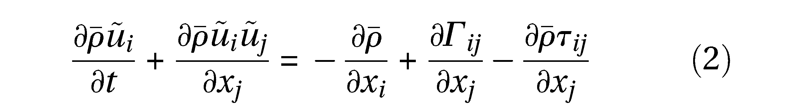
where
There are other aspects of a calculation that separate LES and RANS that are discussed
later. However, at the equation level, the similarity is clear and it is probably best to
view LES as an evolving development of turbulence modelling rather than a completely new
approach distinct from RANS. The equations also point out the importance of the choice one
makes for modelling the term
Turbulence modelling for the term

where

Once again, we arrive at an important observation that equation (3) is used in both LES and RANS
codes. Until a model for
2.1 Expectations of LES
There is a broad perception that LES is an improvement over RANS modelling for engines that is based on several general expectations about LES simulations and results. These expectations are consistent with the general characteristics of the two approaches, and can be important because they help to distinguish between LES and RANS simulations beyond a theoretically based distinction. They also offer a useful method for evaluating LES results that is less formal than full validation against experimental data. These expectations can be grouped into several major categories that are discussed in the following subsection.
2.1.1 More flow structures
One of the primary expectations is that there will be more flow structures, eddies, and vortices represented on the computational grid. Figure 1 shows a comparison of RANS and LES results that illustrates this defining characteristic of LES results. This only serves to demonstrate the difference in results since a proper comparison would require simulating several LES cycles and ensemble averaging the results. The eddies and vortices resolved on the LES grid could be described as turbulence, but in this paper, they will be referred to as flow structures to avoid confusion. The increased flow structures are due primarily to the lower dissipation in an LES turbulence model compared to a RANS model. In terms of equation (3), LES models use a smaller value for the turbulent viscosity, ν T . Correspondingly, there is usually more kinetic energy in the LES flow structures. Increased grid resolution can also play a role in permitting more flow structures on the grid, but as discussed below, this is not always required.

Comparison of (a) RNG RANS and (b) LES velocity vectors to demonstrate more flow structures appearing in the LES on the same computational grid (from [10], reprinted with permission from SAE paper 2003-01-1069, © 2003, SAE International)
2.1.2 Better predictive capability
Another expectation of LES is that it will provide better predictive capability. This is based on the argument that the CFD solver for the resolved scales, ũ i , is doing more of the turbulence calculation using the momentum equation itself, as evidenced by the increase in flow structures. Thus, the turbulence model is required to do less. Since there is more uncertainty in the turbulence model than in the basic equations, the simulations have the potential to be more predictive. However, this assumption is not universally true and can be hard to substantiate and fully validate for LES. Problems and uncertainties in boundary conditions, initial conditions, turbulence models, and grid resolution can contribute to LES results that are not as good as RANS results, even though there is more resolved flow structures.
2.1.3 Interpretation of results is different
The LES framework of spatially averaged terms means that results do not represent ensemble averages. This is advantageous in the sense that new phenomenon can be studied with LES. However, it can be a disadvantage if one is trying to compare to experimental results that are often averaged over many cycles. Proper comparison with experiments requires multiple cycle LES simulations and the related increase in computational time. Users should match the CFD modelling tool to the problem at hand and use LES appropriately.
2.1.4 Easier models
Another possible expectation of LES simulations is that the models involved will use fewer adjustable coefficients and thus be easier to use. This can occur because some LES models are designed to automatically adjust coefficients according to the local flow conditions. This is typically called the ‘dynamic approach’ and was one of the major advances in LES modelling in the 1990s (see [11] and appendix 3). However, another way to understand the reduced number of coefficients is to realize that LES turbulence models are often simpler than the models commonly used in RANS in part because they do not have to account for ensemble average statistics.
2.1.5 More CPU time
A final expectation of LES simulations is that they will require more computer time than RANS models. This expectation is true, but not always to the extent that one may expect. The increase in CPU time reported in many LES studies is due to the greatly increased number of grid points compared to standard RANS grids. This increase is due in large part to the simple and sometimes crude LES models being used. The simple models often require denser grids so that more energy is in the resolved scales and the models play only a minor role. However, a good LES model does not necessarily require a major increase in the number of grid points. For comparable grids, good LES models themselves often require only a modest increase in computer times, typically of the order of 20 per cent longer. The issue of grid resolution and turbulence modelling is important and discussed in more detail in the following section.
2.2 Turbulence modelling
Flow structures and turbulence in general arise from the non-linear terms,
To achieve flow structures in LES, one can choose between crude turbulence models with more grid cells or better turbulence models with reduced grid requirements. The choice of denser grids with simple models is the traditional way to achieve flow structures. However, it comes at the price of increased computational time. The denser grid provides more resolution so that a wider range of resolved length scales are maintained and non-linear interactions are more likely to occur. In this case, it is often acceptable to use simple turbulence models since they are not required to do much other than provide dissipation at the small scales. As shown below, the problem is that often the models are so simple that they provide dissipation over a wide range of length scales, and one is forced to provide even more grid resolution to counteract this effect.
In many situations, the number of cells in a grid could be reduced and the grid would still be sufficient for maintaining a range of length scales and allowing non-linear interactions. However, the turbulence model must allow this to happen. Simply choosing a less dissipative but crude model often will not work because of numerical instability. In addition, reduced dissipation is counter to the concept of LES spatial filtering in which more subgrid dissipation should occur as the number of cells in the grid decreases. Instead, the turbulence model needs to improve as the number of grid cells is reduced. An important characteristic of better LES turbulence models are ones that let the non-linear interactions occur while still maintaining numerical stability.
An example of one such turbulence model is shown in Fig. 2. The model is one of a class known as dynamic structure models described in appendix 4. Several of the dynamic structure models are compared to the two most common LES models used in engines: the Smagorinsky model based on equation (3) and the viscosity-based one-equation model to be described later. The figure shows the power spectra of the transfer term between the resolved flow kinetic energy and the subgrid kinetic energy. This is the energy that is removed from the large scales. The dynamic structure models follow the spectra from the DNS result much better. It is characterized by higher values at higher wave numbers (smaller scales) and lower values at lower wave numbers. In contrast, the Smagorinsky and viscosity-based one-equation models show high values at all wave numbers. This indicates that these models take energy out of the resolved scales (low wave numbers) and reduce the possibility that non-linear interactions will occur and result in flow structures. Thus, a denser grid is required with these types of model to counteract the overly dissipative effect. The dynamic structure model reduces resolved scale energy primarily in the small scales and lets the resolved scale non-linear actions occur.
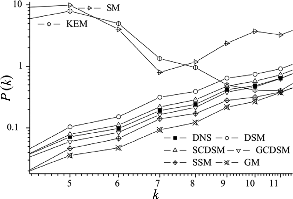
Power spectra of the subgrid kinetic energy production term as a function of wave number for rotating turbulence. DNS is direct numerical simulation, SM is a Smagorinsky model (T2, described in Table 2), KEM is a viscosity-based kinetic energy equation model (T5), SSM is a scale-similarity model, and the rest are all variations of the dynamic structure model (T7) (from [12])
The use of dense grids and simple models goes back to the early work on LES [13]. The initial argument for LES was that the filtering size and hence the grid size should be well into the inertial subrange of an isotropic turbulence spectrum. This also justifies a simpler turbulence model. However, looking more closely, one sees that the inertial subrange requirement was not part of the original LES definition. Originally, LES meant only that spatial filtering rather than ensemble averaging was being used [14]. The requirement for dense grids and inertial range inclusion grew out of the common use of simple, overly dissipative models such as Smagorinsky. This type of approach is still common when LES is used to study more basic or fundamental aspects of turbulence. In those situations, the flow is often for a simple configuration such as homogeneous turbulence. This also allows the use of higher order numerical methods that avoided numerical dissipation.
However, the use of very dense grids in simple flow configurations is a more scientific use of LES and is distinctly different from using LES in applications such as IC engines. Flows are almost never homogeneous in applications. Traditional concepts, such as the inertial subrange, rely on a sufficient statistical population that often does not exist at the smaller scale subgrid level in a complex evolving flow. In engine applications, it is not practical to use extremely dense grids or higher order numerical methods. The domain size and configuration do not allow it. In addition, the more complex physical processes, such as combustion and sprays in engines, require their own modelling and computational time. Thus, most practical LES applications for engines must use coarser grids and lower order numerics.
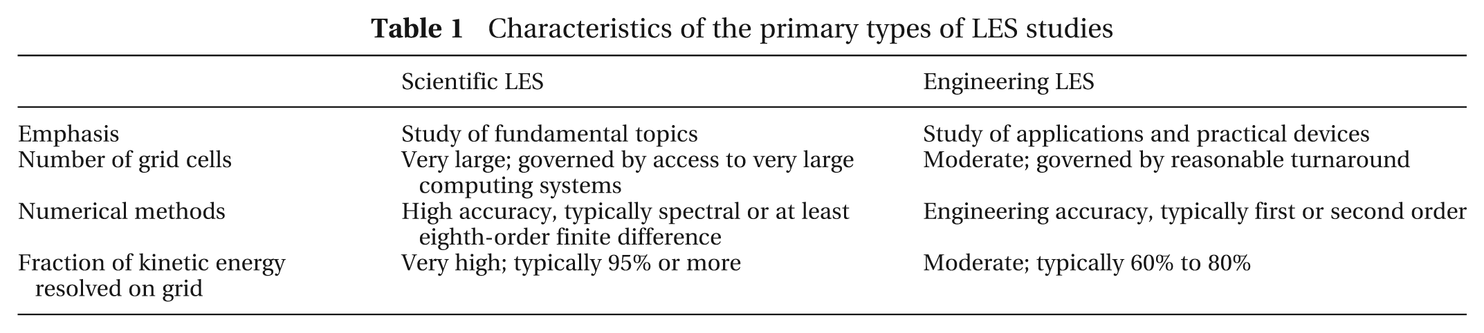
To account for the different types of LES, the notation ‘scientific LES’ and ‘engineering LES’ is introduced. Some of the characteristics of these two types are listed in Table 1. Since the motivation and objectives of the two types of LES are different, each should be evaluated within their own context. For example, engineering LES must contend with errors and added dissipation arising from lower order numerical methods. This is somewhat countered by the higher values of subgrid kinetic energy in engine LES. This is indicated by the fourth item in Table 1, and is similar to the LES quality index introduced by Pope [7]. Larger values of subgrid kinetic energy mean that numerical dissipation is a smaller fraction of the subgrid values and the relative impact of numerical errors in engineering LES is potentially less significant. However, this places more reliance on the subgrid models. Generally, knowledgeable users are able to incorporate these characteristics of engineering LES into their interpretation of results and analysis.
Characteristics of the primary types of LES studies
An example of how LES can be used in a CFD code designed for engine applications is shown in Fig. 3. This shows experimental, RANS, and LES simulations of the Sandia Cummins direct injection diesel engine. The RANS and LES simulations duplicate the region of the experimental images using the same coarse grid of a simple sector mesh common in diesel engine simulations. The RANS results show a broadened or smeared region for the higher temperature, while the LES results show the same type of jet large-scale structures seen in the experimental images. Thus, with only a change to LES turbulence and scalar mixing models that are appropriate for applications, the simulation results pick up flow processes that occur in the experiments that were not previously available in the RANS simulations.
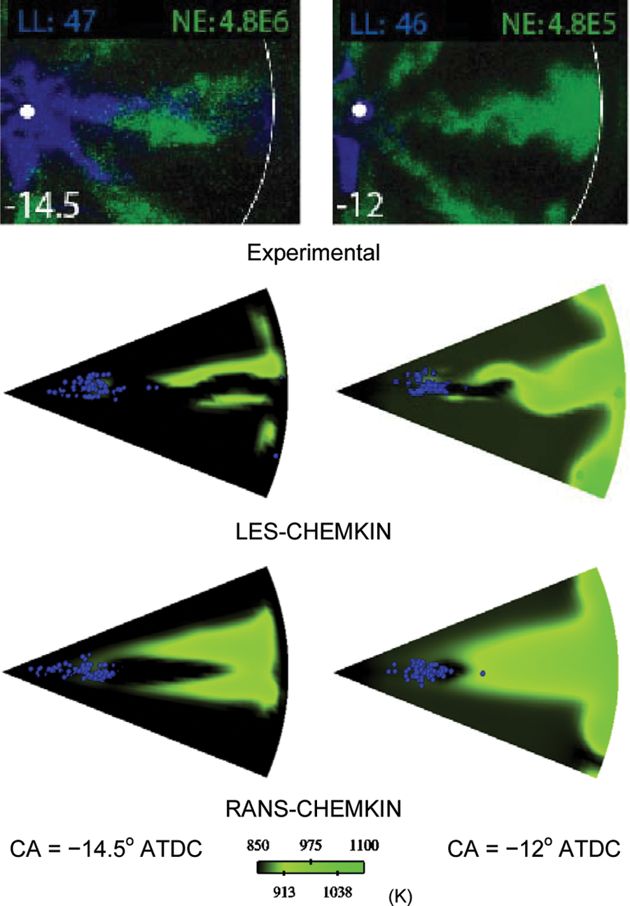
Comparison of LES (middle row) and RANS (bottom row) with experimentally imaged (top row) ignition chemiluminescence, showing liquid fuel in blue and temperature in green (see scale) (from [15], reprinted with permission from SAE paper 2007-01-0163, © 2007, SAE International)
2.3 Expectations of LES for IC engines
In addition to the general expectations of LES listed above, there are additional expectations related to IC engine simulations. Generally, these can be described as the ability to study new physical phenomena in engines and an increased sensitivity to design changes. These are discussed in more detail in the following subsection.
2.3.1 Study new phenomena
A very important aspect of using LES for engines is that it will allow studies of new phenomenon. There are important aspects of engine flows and combustion that are difficult, if not impossible, to address with RANS but which are more amenable to LES approaches. One of the primary features is cycle-to-cycle variability. Reynolds Average Navier Stokes uses models designed to capture the ensemble averages. This results in higher turbulent viscosity that almost always removes, or at least smears out, the variation of in-cylinder flows and combustion that coincide with cycle-to-cycle variability. Since LES models are designed to filter out the smaller scales and retain the larger scales, they are less dissipative. The remaining large scales respond to the non-linearities inherent in the Navier Stokes equations, and at least some aspects of cycle-to-cycle variability can occur in the simulations. As discussed in section 4, several research groups are already making use of LES to study cycle-to-cycle variations.
2.3.2 Increased design sensitivity
In addition, there are other flow-based processes in engines that are best addressed with LES rather than RANS. For example, LES should be better at capturing the impact of relatively small changes in geometry (combustion chamber shape, pistons bowls, port design, valve curtain regions, etc.), small changes in fuel injection angles for direct injection applications, and small changes in operation (spark timing, injection timing, valve timing, etc.). These types of applications could be classified as ‘design sensitivity’ studies. Similar to cycle-to-cycle variability applications, LES is a necessary tool for these studies due to its increased sensitivity.
Even though LES represents the next generation of turbulence modelling, it is not always the best choice for engine applications. The primary and very common situation in which RANS is still the best choice is when the desired output is a cycle-averaged result. Obtaining a cycle-averaged result with LES requires running several consecutive full 720 crank-angle degree cycles and averaging the results. This can be expensive since additional grid preparation is required for the open portions of the cycles and computer run times are long for the ten or more cycles required. Several research groups are pursuing this approach (see section 4). One justification for this more computationally expensive approach is that LES results are more accurate so that the average is better than a RANS result. Still, users should evaluate their objectives and choose the best approach, either RANS or LES.
The other significant reason that LES is at a disadvantage for engine applications is that many additional complex physical processes occur. Combustion and fuel injection are probably the primary complicating processes, and these are not trivial. The use of LES for turbulent combusting flows is still a very active area of fundamental research with many basic issues still being investigated [16]. There has been even less work in LES for liquid sprays where one could easily argue that the physical processes are even more complex. Beyond sprays and combustion there are complex processes in ignition, gas phase and solid phase emissions, boundary layers and wall heat transfer, and moving boundaries. All of these require some sort of modelling that should be adapted, or at least understood, for the LES approach.
In many situations, researchers use LES for turbulence (e.g. subgrid stresses that appear in the momentum equation) and maybe for scalar flux modelling, but then rely on existing RANS-type submodels for the other physical processes. This type of hybrid approach is very common and a very reasonable way to proceed. Waiting until all engine submodels have been adapted to LES is unreasonable and disregards the advantages that can come from intelligent use of hybrid approaches. Since turbulence is the background for most aspects of engine flows, using LES turbulence submodels can improve the context for the other models. The turbulence models provide flow fields with more large-scale structures and greater sensitivity so that many advantages of LES can be realized, even when combined with RANS models for other processes. One could argue that there is some justification in this approach since RANS models for combustion and sprays should respond correctly to the resolved large-scale flow field [17]. However, the correct response of RANS models to the LES flow field is not guaranteed. A user should understand the specifics of the hybrid situation being used so that they can better evaluate the appropriateness of the tools for the specific study and the validity of the results. An even better approach is to examine the various submodels and determine if they are consistent with the LES spatial filtering concepts and the resulting scaling.
This brings us to the main objective of this review, which is to report on, evaluate, and categorize the use of various LES turbulence, combustion, spray, etc., models for IC engines. Since there are many physical processes that need modelling, there is a wide variety of hybrid approaches in the literature that may mix-and-match various models from these lists. Examples from the literature will be used to illustrate some of the main categories. Then, these categories are used to describe and classify some of the recent uses of LES to study engines.
3 LES Models in IC Engines
There are many complex physical processes in IC engines, and each of these requires some sort of modelling. These processes occur in a turbulent gas phase flow so turbulence models, also called turbulence submodels, provide the context for the other physical processes. In addition, LES submodels should also be used for scalar mixing, combustion, and fuel sprays since all of these can be significantly impacted by the turbulent flows. Large-eddy simulation modelling for turbulence and these other engine processes are discussed in the sections below. In each case, the major modelling approaches are described and classified with an emphasis on their suitability for engine CFD. A table is provided in each subsection to summarize the descriptions.
3.1 Turbulence modelling
For a quick background on turbulence modelling, one can start from the gradient assumption used in equation (3), although as explained below, this is not necessarily the best approach. From equation (3), the turbulence model is based on a turbulence viscosity, νT, and an expression for this term is required. As a context for the LES approach, the most common RANS-based models use the k–epsilon (k–ε) approach so that

The terms k and ε are interpreted to be the turbulent kinetic energy (TKE) and the turbulent kinetic energy dissipation rate (or just dissipation). In modern approaches, these terms are obtained from individual transport equations. Thus, the RANS (k–ε) model is a two-equation turbulence model.
To provide additional understanding, it is useful to rewrite the model based on a physical interpretation using a velocity and length scale

Then, k and ε provide a turbulent velocity scale
If equation (3) is used for LES models, there are several approaches for obtaining expressions for νT. One of the more common models is based on the ideas of Smagorinsky [18] and results in

where
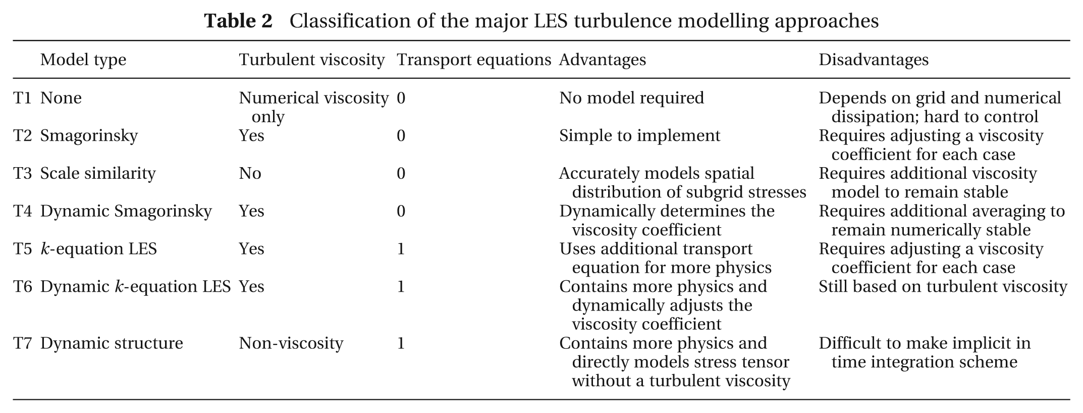
Classification of the major LES turbulence modelling approaches
Within the turbulent viscosity approach to modelling, the LES model length scale is related to the grid cell size. This means that fundamentally LES is not grid independent. As the grid cell size becomes smaller, an LES solution should approach a DNS solution. This limit is well accepted and usually realized by most LES models. In contrast, as the grid cell sizes become larger, the limit is not well established. One possible interpretation is that the LES model length scale should approach a RANS model integral scale. However, this is not observed in practice and, pragmatically, it is inadvisable to use LES models on grids coarser than ones used in RANS.
Even though most turbulence models use some form of equation (3), it can be argued that it is not the best type of model for LES for three important reasons.
Overly dissipative. As discussed in the previous sections, this approach can be overly dissipative.
No subgrid kinetic energy. In equation (3) type models for LES, the
subgrid TKE is arbitrary. This is because the trace of the subgrid stress tensor,
τ
ii
, is twice the kinetic energy, but the trace of the
strain rate tensor is zero in incompressible flows. This is why equation (3)
uses the anisotropic part of the subgrid stress tensor,
Incorrect tensor relationship. Fundamentally, equation (3)
assumes the tensor relationship between
Table 2 classifies the major approaches to LES turbulence models and briefly states advantages and disadvantages. This is followed by more detailed discussions of each type of model. This table does not list more esoteric or academic models, but includes only modelling approaches that are likely to find use in engine applications. Note that this table is only for simple turbulence (e.g. no scalars, sprays, combustion, etc.).
T1. The simplest turbulence model is no model at all. This approach relies on very dissipative numerical methods to replace the turbulence model (see, for example, [20]). Somewhat surprisingly, this approach can give realistic results, mainly because the characteristics of numerical dissipation are similar to those of viscosity. However, it is generally viewed that one should explicitly represent the subgrid effects rather than relying completely on numerical properties. This is particularly true in flows with complex physics such as engines. Thus, this approach is not recommended.
T2. The Smagorinsky approach was the first LES turbulence model and has already been described previously in equations (3) and (7). It is an algebraic (e.g. zero-equation) turbulent viscosity model. There is a model coefficient, CS, in the turbulent viscosity term of equation (7) that must be specified. In simple Smagorinsky, the coefficient must be adjusted for each simulation situation. The model is very dissipative and requires fine grids to obtain good results. Since the model is easy to program, it often appears as an option in commercial CFD codes. The Smagorinsky model is fairly common in engine simulations, but the dense grid requirement is usually too restrictive and better models exist.
Celik et al. were some of the first researchers to explore LES in engines [21]. Their work used the T2 turbulence model in the KIVA code [22] and simulated intake and compression flows in diesel-type cylinders. Despite being originally developed for RANS models, results from KIVA demonstrated that it was capable of capturing large-scale flow structures. A review of the early work in engine LES helped to increase awareness of using LES in engines [23].
An additional variation associated with T2 type models was developed by Nicoud and Ducros [24] and called wall adapting local eddy (WALE) viscosity. This replaces the strain rate magnitude in the turbulent viscosity in equation (7) by a more complex tensor contraction of the strain rate and velocity gradient tensor. There is some indication WALE has better near-wall performance so that grid requirements can be reduced, but this needs further investigation. Poinsot, with a variety of other researchers, has used WALE with non-engine flows in the development of a new code for engine applications [25, 26]. Bianchi et al. have shown good results with WALE in engine flows with a detailed analysis of flow around the intake valves [27, 28].
T3. The scale-similarity modelling approach was originally proposed by Bardina et al. [29], and is explained in more depth by Meneveau and Katz [30]. The concept is that unresolved subgrid scales can be approximated by the smallest resolved scales. In other words, the best way to represent subgrid scales is with the next largest scales. This approach is implemented by using an additional spatial filtering operation on the already filtered scales. The additional filtering may be called a test filter in some approaches and is indicated by an additional overbar-type symbol (see appendix 3).
Scale-similarity is an important concept in LES and does not occur in RANS modelling. The original approach is usually unstable, mainly because it is not a viscosity model and does not use an energy budget to track the subgrid kinetic energy. Thus, the scale-similarity model is usually augmented by the addition of a Smagorinsky term in what is termed a hybrid model.
The Lund University group has been exploring LES for engines for several years using a scale-similarity model for turbulence. A lot of their work is focused on homogeneous charge compression ignition (HCCI) combustion, and is reviewed in section 4. They worked with Paul Miles from the Combustion Research Facility at Sandia National Labs to make detailed comparisons of motored in-cylinder velocity fields [31]. They used dense grids, and the comparisons between the LES and the PIV are reasonable. Interestingly, the work demonstrates the difficulty in validating the LES.
T4. A major improvement in the Smagorinsky approach occurred when the dynamic approach was developed by Germano et al. [11]. In this approach, the adjustable coefficient, Cs, in equation (7) is obtained using the dynamic procedure. The dynamic procedure uses the scale-similarity concept of T3 that requires an additional spatial filtering step. The dynamic coefficient is found from the difference between these additionally filtered quantities and the base quantities calculated on the CFD grid (see appendix 3). This additional filtering operation is a modest increase in computational cost, resulting in an increase of ~20 per cent for a simple turbulent flow.
An interesting variation of the dynamic procedure was developed by Meneveau et al. [32], in which a Lagrangian concept was used to develop the model coefficient. The idea was to average over fluid particle pathlines to improve accuracy. In practice, two additional transport equations were used to represent the Lagrangian average of terms used to evaluate the dynamic coefficient.
Haworth et al. were also some of the early explorers in using LES for IC engines [33]. They mostly used T2 and T4 type models in several different codes. They carried out extensive studies on a simple, engine type flow with a stationary valve [34]. This configuration, sometimes called the Imperial College engine, has a large experimental dataset and is useful for validating valve flows. Haworth et al. have shown good comparison between ensemble averaged LES models and experimental data for both mean and fluctuating velocity profiles at different locations and different crank angles.
The dynamic procedure is very powerful and can be used in many situations to find modelling coefficients. When used with the Smagorinsky model, the results are reasonably good for non-reacting flows. However, dense grids are required and often an additional averaging must be used to avoid instabilities that arise from negative viscosities. Despite the improvements found in T4, it still retains the drawbacks of the equation (3) viscosity models discussed in the previous section. No matter how good a model is formulated for the turbulent viscosity, the fundamentals of T2 and T4 are very weak.
T5. The k-equation approach is a practical
viscosity-based, one-equation LES model. It was originally developed for atmospheric flows
[35], and is still common in
that field. Some of the first useful k-equation models for engineering
flows were developed by Kim and Menon [36]. This model was still viscosity based (equation (3)), but now the turbulent
viscosity was formed from the subgrid TKE, ksgs, and a grid
length scale,

The subgrid TKE was obtained from an additional transport equation that was readily derived from the basic equations. The use of the k transport equation has several distinct advantages. First, it incorporates more physical processes, such as the convection, production, and dissipation of subgrid kinetic energy. Second, the subgrid kinetic energy provides a velocity scaling that can be used in other models, such as combustion, scalar transport, and sprays. Third, models that use a subgrid k-equation provide a better model for the subgrid stresses and thus work better on the coarser grids commonly found in engine CFD [37, 38].
Menon et al. have applied the T5 turbulence model to engine flows with good results [39]. Bianchi et al. have performed careful studies of LES models for engine type flows in simple configurations. For example, they have compared T2 and T5 turbulence models with RANS results for a stationary valve, steady flow bench configuration [28].
The subgrid kinetic energy equation is fairly simple to implement. It requires only one additional major modelled term, which is for the dissipation of subgrid kinetic energy. Fortunately, this term plays its proper role in LES, which at the subgrid scale is to remove kinetic energy. The dissipation term is not required to provide the mean value for all scales, nor is it used to obtain length scales or time scales as it is in RANS modelling. Thus, dissipation modelling is much less critical, and simple models seem to work well.
T6. The k-equation LES models have also been implemented using the dynamic procedure to obtain a better, local value for the coefficient in equation (8) [36]. This method is a logical extension of T5; however, additional implementation details must be observed to maintain stability. At this time, it is not clear if this additional complexity beyond the basic T5 model is useful in engine simulations.
T7. A recent development in LES turbulence models is the dynamic structure approach developed by Pomraning and Rutland [40] and Chumakov and Rutland [41]. In this approach, a turbulent viscosity is not used. Instead, a tensor coefficient is obtained directly from the dynamic procedure. This tensor coefficient is multiplied by the TKE that is obtained from a transport equation (see appendix 4 for more details). The resulting dynamic structure model is

An important major aspect of the dynamic structure approach is that there is no turbulent viscosity. Thus, it is not a purely dissipative model. Instead, a budget of TKE is maintained between the grid scale velocity field and the subgrid k-equation. In other words, energy removed from the grid scales goes into the subgrid kinetic energy. Then, within the k-equation, a viscous dissipation term removes the energy through molecular viscosity. Detailed a priori and a posteriori testing of the model has shown it performs well in rotating turbulence in which energy is transferred accurately from small to large scales, a process that is similar to that occurring in sprays and combustion systems [12, 42].
The model was developed for practical applications, especially IC engines, in which the number of grid cells must remain reasonable. The model works very well in engine applications, and provides a good model for the subgrid TKE for use in combustion, scalar mixing, and spray models. The T7 approach has been used for diesel engine simulations with good results [15, 43, 44].
3.1.1 Turbulence: additional considerations
Wall boundary conditions. Wall boundary conditions for LES submodels are not very well developed. There has been continued effort is this area for several years (e.g. Kannepalli and Piomelli [45] and Chang et al. [46]), but, to date, no significant progress has been made on practical models for CFD applications. Some promising advanced work by Cabot and Moin [47] used RANS models with additional consideration for unsteadiness and ‘ejection’ events. However, these have only been used on simple channel flows and will probably require much more additional testing before they can be used with confidence in applications. More recently Piomelli [48] has reviewed the status of wall modelling for LES, and Fröhlich and von Terzi [49] discussed combining LES with RANS wall models.
Thus, most LES simulations use one of two approaches for wall boundary conditions: (a) no special treatment of the wall, except for additional grid points (Kannepalli and Piomelli [45]), and (b) wall-layer models essentially the same as used in RANS that have been shown, by Rodi et al. [50], to give reasonably good results. For engine applications, the use of wall functions is probably the best approach for the near future. This is especially true when one considers wall heat transfer for which there has been essentially no work on engines for LES specific wall models.
Higher order numerics. In simulations that are less focused on applications and more focused on generic flows, such as channels and isotropic turbulence, numerical accuracy is an important issue [51]. The concern is that numerical errors could be of the same order as the LES modelled terms. The generic flows commonly use higher order spatial numerics, typically fourth order or higher. In addition to being higher order, the methods have low dispersion and dissipation errors. This is possible because the computational domains are simple and the grids allow easy implementation of higher order numerics. In contrast, applications such as IC engines commonly have complex grids and it is very difficult to achieve anything higher than second-order spatial accuracy. This should not and has not deterred the use of LES to achieve better results in engine applications.
There has been encouraging work by the group at Doshisha University to improve the numerical accuracy in the KIVA engine applications code [52, 53]. This work correctly focuses on the advection or convection term in the momentum equation and has compared several numerical methods, including one that is up to third-order accurate. The results are encouraging, but have only been demonstrated on simple grids in the engine code and have not been demonstrated on grids for actual engine configurations.
Another tactic for higher order accuracy is being used by Poinsot et al. at IFP and CERFACS, in which an existing LES code developed for aeronautical applications is being adapted for IC engines [25, 54]. The code is known as AVBP, and has second-order time accuracy and third-order spatial accuracy on the convection terms. The time integration scheme is explicit, which offers higher accuracy than an implicit scheme since the time step is restricted to smaller values. Adaption for engines is not straightforward, but moving mesh algorithms have been implemented; however, grid removal does not seem to be included yet. The code is being carefully tested and is showing good results for engine applications [55].
Compressibility effects. Even though the gas density varies significantly in engines, they are generally considered low Mach number regimes [56]. Thus, pressure wave effects on turbulence modelling are almost never considered. The exception is when engine knock or extremely rapid ignition occurs. While some HCCI operation is similar to knock, it can be considered a different mechanism that is probably not a consequence of pressure waves in most cases. There are many RANS-based studies of knock (see, for example, [57]) but there does not appear to be any LES studies yet. This will probably change before long as ‘mega knock’ in downsized [58] or direct injection gasoline engines is studied.
Open boundary conditions. Many engine studies are focused on the closed portion of the cycle and thus avoid open boundaries. However, as multicycle simulations become more common to study topics such as cycle-to-cycle variability, inflow and outflow boundary conditions must be considered. It is not always clear what information should be specified on the boundaries to achieve accurate simulations. One LES study found that boundary flow perturbations can have a significant impact on combustion [59]. This topic needs additional study, and it is likely that the type of engine, the specific models being used, and the focus of the investigation will have an impact on what boundary conditions are required.
3.1.2 Turbulence: recommendations
The use of LES for basic turbulence modelling in applications is becoming better established and can be used for engine CFD with the appropriate models.
The most common LES models use simple viscosity formulations (T2, T4) and do not take advantage of LES concepts. They require high grid resolution, which can be achieved using highly parallel codes.
The more advanced differential LES turbulence models (T5–T7) should be used. These do not require extremely fine grids and work well on the grids commonly found in engine applications.
Models that use a subgrid TKE, ksgs, are well suited to engines because this term can be used in modelling combustion, scalar mixing, and sprays.
3.2 Combustion modelling
The phrase ‘combustion modelling’ refers to modelling the chemical reaction rate terms in the energy and species conversation equations. Often, these models incorporate additional transport equations for mixture fraction or flame surface expressions. These additional equations may require additional models for terms such as scalar dissipation or turbulent flame speeds. Combustion modelling is a complex and evolving field. Readers should consult reviews by Pitsch [16], Menon [60], Veynante and Vervish [61], Hilbert et al. [62], and the book by Poinsot and Veynante [8] for detailed background information. In this section, the major combustion models that are used or have potential application for IC engine CFD are classified and briefly described.
In almost all cases, the combustion models are essentially RANS models that have been or could be adapted for use in LES. This approach clearly treats LES as an evolution of RANS modelling and seems to work well. The combustion models benefit from the LES flow field and scalar mixing models. In addition, as noted by Kempf et al. [17], the RANS formulations, though originally based on ensemble averaging, may still be appropriate for LES-based spatial averaging and respond correctly to the LES flow field. However, the best approach is to re-evaluate the models and make appropriate modifications to be consistent with the LES approach. This adaptation may be as simple as adjusting coefficients within the original RANS model. Or they may be more complex and require reformulation of the expressions to be consistent with the time scales that are available from the LES turbulence and mixing models. For example, specific LES formulations of scalar dissipation models may be required in mixture-fraction-based combustion models (see, for example, [63]).
Table 3 classifies and briefly describes the major approaches to combustion modelling that have either been used or could be used for engine CFD. Some of the models have been grouped into families with specific approaches listed as subcategories.
List of major combustion modelling approaches that have potential for use in LES. Original or primary type of combustion for each model is indicated by Mode in column 2: H for homogeneous, P for premixed, D for diffusion
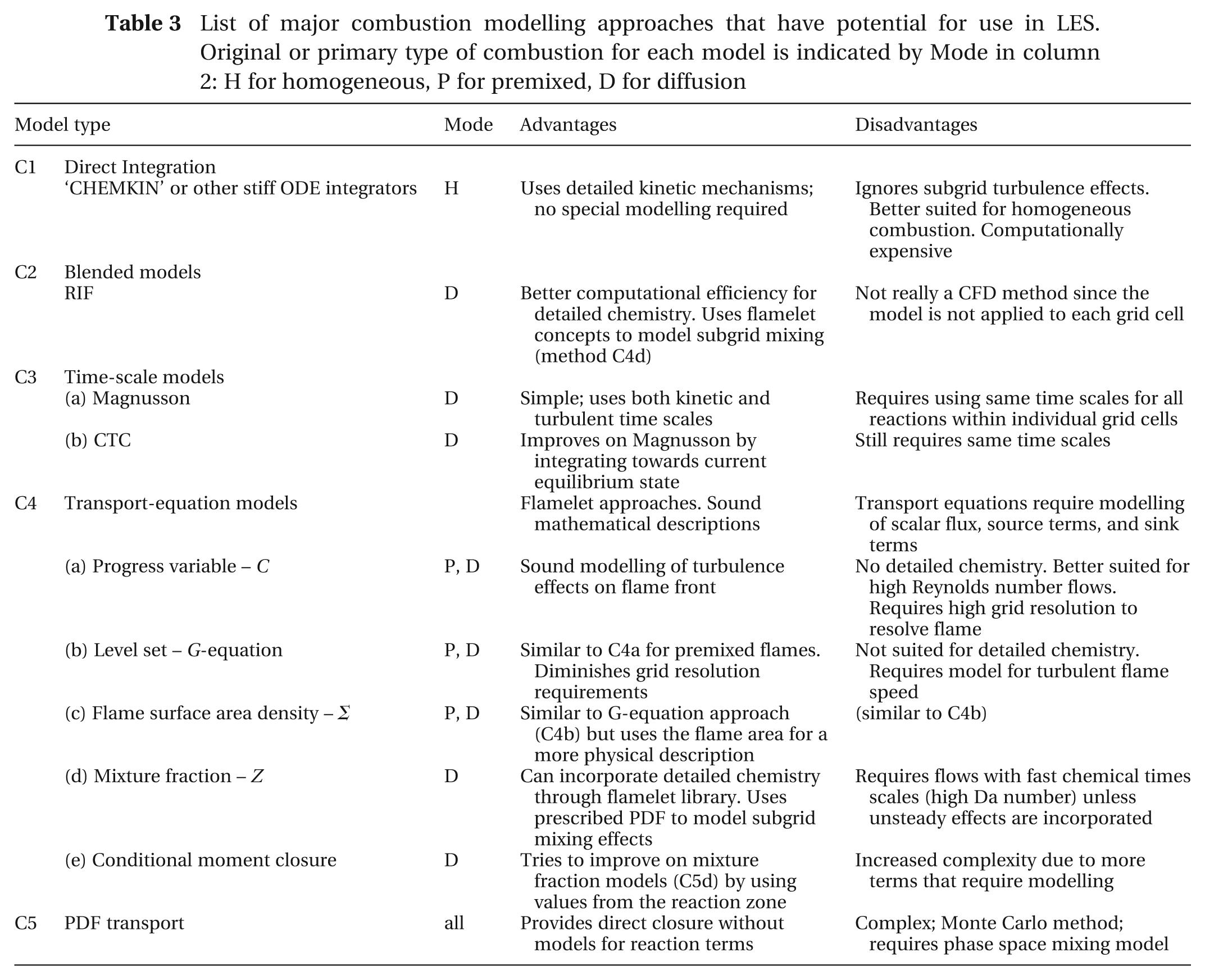
C1. The direct integration approach is also called the mean-flow approach since reaction terms are evaluated using the grid scale (e.g. filtered) temperature and species. These do not account for subgrid mixing effects, so they are best suited for more homogeneous flows and detailed chemical kinetic schemes. Alternatively, direct integration is suitable for dense grids when the subgrid values are Gaussian with small variance. This approach has proven to be very successful for studying low-temperature combustion (LTC) approaches such as HCCI. For example, Reitz and his group have successfully applied C1 modelling for RANS modelling in direct injection and homogeneous charged LTC diesel engine studies [64], gasoline direct injection engines [65], and in similar dual-fuel combustion strategies [66]. The approach has also been used successfully in LES applications using the T7 turbulence model for direct injection diesel LTC studies by Rutland and his group [15, 43, 44].
The C1 approach requires detailed chemical kinetic mechanisms to be successful in engines, and this usually results in very large computational run times. Progress in improving run times is being achieved by improved load balancing in parallel computing environments [67]. Additional run-time improvements are being achieved by applying advanced numerical techniques such as cell clustering and analytical Jacobians [68] or precomputed, tabulated results from detailed chemistry calculations [69, 70]. These methods are computationally efficient, but may require close monitoring of approximation errors, especially for ignition and other situations where results are sensitive to kinetic details.
C2. In an attempt to incorporate more detailed chemical kinetics but without the computational penalty, Peters’ group have developed the representative interactive flamelet (RIF) model [71–74]. Individual ‘flamelets’ that represent the main combustion process are tracked using a Lagrangian method through the domain. The approach can be calibrated to work with conventional diesel combustion and provide detailed chemistry for emissions. However, the approach has difficulty with more homogeneous flows, wall heat transfer, multiple fuel injection operation, and spatially non-uniform mixing that can occur in different regions of the combustion chamber. Additional flamelets are sometimes added to help address these issues, and the method begins to resemble the cell clustering approach used in C1 models. Combustion is tracked by the Lagrangian flamelets rather than the processes within each CFD grid cell. The approach is more of a blending between a CFD flow model and a system level heat-release model. Since it is not clear how a representative flamelet concept is consistent with the LES spatial filtering approach, the RIF approach is not recommended for LES.
C3. For RANS applications, the time-scale approach was originally developed for spark ignition engines (Abraham et al. [75]) and later adapted for diesel engines (Kong and Reitz [76]). The characteristic time-scale (CTC) model is a very practical approach that can give good results when experimental data are available to adjust coefficients. The CTC model is an outgrowth of the less commonly used Magnusson type approaches, but is more advanced in that CTC drives species concentrations to a specified value. This specified value is commonly the local equilibrium value. However, in some models this specified value is obtained from a strained laminar flamelet solution (see, for example, Rao and Rutland [77]). This effectively combines the flamelet-prescribed PDF approach (C4d) with the time-scale approach and has been used successfully with LES turbulence models in diesel engine simulations [78].
C4a. The flame-sheet approximation for premixed flames has been developed in two formulations: the C-equation and the G-equation approaches originally developed by Bray [79] and Kerstein et al. [80], respectively. However, as shown by Zimont [81], the approaches are very similar. In the C-equation approach, the RANS flame brush is represented by a progress variable C (commonly normalized temperature). This flame-sheet approach has been extended by Zimont et al. [82] for RANS simulations.
The group at the Lund University has published a series of papers using a progress variable approach with a very highly resolved T2 turbulence model [31, 83–85]. Their work was focused on understanding HCCI and they achieved good comparisons with experimental pressure traces. Figure 4 shows an example from one of their LES simulations. Additional discussion of their work appears in section 4.

Instantaneous temperature fields from an HCCI test engine with a square bowl designed to increase turbulence levels (from [85], reprinted with permission from SAE paper 2008-01-1656, © 2008, SAE International)
The adaptation of the C progress variable model for LES has shifted away from the RANS moment-based approaches towards a simpler formulation called the thickened flame model [86]. This is a simple concept that artificially increases the flame thickness and is motivated by reducing the computational time used in the combustion model. This allows denser grids and more resolved scale motions that work well with the thickened flame. Researchers in France have made good use of this approach in LES and have simulated multiple cycles of a spark ignited premixed charge compression ignition (PCCI) engine [55].
C4b. The G-equation approach uses a continuous variable, G, but assumes that a specific line of constant G represents the flame front. It is a level-set, kinematically based approach and is extended to combustion only by the concept of a flame sheet. The function G evolves by a standard transport equation that requires models for the subgrid scalar flux. This approach is being developed for RANS simulations (see summary in Peters [87]). It also shows some promise for use in LES simulations of premixed flames [88]. More recently the G-equation approach has been formulated for diffusion flames and used in diesel engine simulations by Yang and Reitz [65]. These simulations use RANS modelling, but the extension to LES should be straightforward.
C4c. The flame area per unit volume approach was originally developed for diffusion flames by Marble and Broadwell [89]. It was later adapted for premixed flames in RANS simulations by Candel and Poinsot [90] and Ducros et al. [91], and is commonly called the coherent flamelet model (CFM). The flame surface density, Σ, is used with a laminar flamelet solution to obtain the total reaction rate in a CFD cell. Commonly a transport equation is used to obtain Σ. This requires modelling of the scalar flux and additional source and sink terms specific to flames sheets. These source and sink terms are key components for accurate predictions.
For engine applications, the coherent flamelet has been used in RANS simulations by Angelberger et al. [92], Henriot et al. [93], Colin et al. [94], and Colin and Benkenida [95]. More recently, the approach has been expanded for RANS engine simulations and called the ECFM and ECFM3z methods [96–98]. The CFM approach was adapted specifically for LES by Weller et al. [99] for premixed flames in non-engine applications. For LES engine applications, the CFM model was adapted for diesel combustion and used by Musculus and Rutland [100] and the ECFM-LES method was developed by the researchers at IFP, the EM2C laboratory at Ecole Centrale Paris, and the CERFACS organization [59, 101] (see section 4 for additional discussion).
C4d. The LES versions of the mixture fraction approaches are very similar to RANS models – the mean and variance of a conserved scalar (usually mixture fraction) are used to build an assumed PDF. This PDF is then used to obtain mean quantities from laminar flamelet solutions. In general, the solutions are not very sensitive to the shape of the PDF and beta functions are the most commonly used PDF. The mean of the scalar is usually obtained from a transport equation that requires mixing models (e.g. scalar flux models; see following section). The variance of the scalar can be obtained from either another transport equation or from an algebraic closure by equating scalar production and scalar dissipation. Either method requires the scalar dissipation. This approach has been used successfully by many people for non-engine LES combustion models [69, 102–106]. The mixture fraction approach also works well with LES in engine applications (see, for example, [15, 78, 107, 108]).
C4e. The conditional moment closure (CMC) is a variation of C4d in which many terms are supposed to be evaluated at the reaction zone (e.g. a conditional evaluation). The objective is to resolve local mixing conditioned on the mixture fraction. The model was originally developed for non-premixed flames independently by Klimenko [109] and Bilger [110]. The approach expands the mixture fraction models by using a conditional averaging approach so that many terms in the transport equation use values at the reaction front. Most of these conditional terms require additional assumptions and modelling, so CMC can be more complex and computationally expensive than conventional mixture-fraction models. The CMC approach has been used in RANS simulations of engine-like flows [111, 112] and in diesel engines [113]. The CMC approach has been adapted to LES for non-engine flows (see, for example, Steiner and Bushe [114]), but it is not straightforward, as shown by Triantafyllidis and Mastorakos [115]. Generally, results with CMC are usually slightly better than a typical C4d model. However, the CMC complexity and lack of general experience that comes from wider use indicate that the approach still needs development for use in LES of complex engine flows.
C5. An additional combustion modelling approach is based on the PDF evolution equation models. The approach is often referred to as the ‘transported PDF’ approach as opposed to the ‘presumed PDF’ approach in C4d and C4e. The theory was originally developed by Pope [116], primarily for RANS environments. A recent review of this method by Haworth [117] provides detailed information about the physics, mathematics, and numerical details of this approach, including a section on its use for engines. This is a complex approach using Monte-Carlo methods to track the evolution of the underlying PDFs that describe the thermal and, in some cases, velocity fields. The primary advantage of the approach is that it does not require any additional models for the chemical reaction terms. However, it does require models for subgrid turbulence and phase space mixing. The method is so different from the other approaches discussed here that some users find it difficult to use. Since it is a statistical approach, the method can require long CPU run times. However, Subramaniam and Haworth [118] and Kung and Haworth [119] are actively developing the method for IC engine application and are achieving good results in RANS simulations. There is little LES work with the transported PDF approach and there does not appear to be any published applications of the models to LES engine simulations to date.
3.2.1 Combustion: additional considerations
Time scales. Combustion models in LES require good models for mixing of species and/or thermal energy. Large-eddy simulation is well suited to provide better mixing information in support of combustion models, especially at the grid scale. At the subgrid scale, combustion models require time-scale information in one form or another (mixing times, scalar dissipation, kinetic times, etc.). Currently, LES models are less well suited to this task because there has been less development on models that provide this information. Often, subgrid time-scale information is obtained from turbulent viscosity and local mean gradients, but this is based on RANS concepts. The newer one-equation turbulence models (T5, T6, T7) are better at providing time-scale information because they track the subgrid kinetic energy ksgs using a transport equation. This can be combined with length scales (gradients or filter length scales) to provide time scales to combustion models.
Multimode combustion. In some engine applications, combustion does not easily fall into the traditional classifications of premixed mode or non-premixed mode. Or combustion may occur in multiple modes within a cycle. Examples are direct injection gasoline technologies and some of the newer LTC technologies such as partially PCCI. These types of combustion processes are probably best described by combinations of direct integration for ignition (C1), premixed and partially premixed combustion for early, more highly mixed processes (C3, C4a–c), and mixing controlled combustion for later processes (C4d–e). These multimode operations can occur in a time sequence, or simultaneously, but in different regions in the combustion chamber, or some combination of these two situations. A combination C4a and C4d model for non-engine LES was reported by Ihme and Pitsch [120]. For engine applications, hybrid approaches have been explored for RANS diesel applications [107] and premixed/diffusion combustion in the ECFM3Z model [95]. More recent work has demonstrated LES simulations of diesel engine simulations using a combination of C1, C3b, and C4d combustion models with a T7 turbulence model [15, 44].
The difficulty with multimode approaches is designating and accurately evaluating the best parameters for switching between the modes. Commonly, these parameters measure a mixing state (for example scalar dissipation rate), relative timescales (Damkohler or Karlovitz numbers), or reaction progress (for example, reaction products or normalized temperature). Currently, there is not a good theoretical framework for determining the switching parameters, so they are often developed based on physical arguments. In addition, the switching procedure and the value at which the switch occurs may have a greater impact on the results than the details of the individual combustion models. Clearly, much more work needs to be done in this area for both RANS and LES modelling.
3.2.2 Combustion: recommendations
Use transport-based combustion models (C4). The transport equations in these models benefit from the large-scale flow structures that occur in LES simulations.
Use LES specific modification for major terms within the models such as mixing time scales, scalar dissipation rate, turbulent flame speeds, scalar flux, etc.
Use a k-equation-based turbulence model (T5, T6, T7) that can provide a subgrid TKE to the combustion model.
3.3 Scalar transport and mixing
Reacting flows require simulation and modelling of scalars such as species concentrations and thermal energy. Since it is becoming more common to use larger, more detailed chemical kinetic mechanisms, there can be a large number of species, and each one requires its own transport equation (see, for example, Tamagna et al. [121, 122]). There are usually source terms in these equations from the chemical reactions, but these are modelled by the combustion models described in the previous section. Beyond this, the primary modelling requirement is the subgrid scalar flux term that comes from spatial filtering the non-linear convection term in the transport equations (see equation (14)). In the future, as fine grids and detailed kinetic mechanisms become more common, complex molecular transport and Lewis number effects may need to be considered.
Subgrid scalar flux or turbulent scalar mixing is physically and mathematically similar to turbulent subgrid stresses (equation (12)). As a result, models for scalar mixing are often extensions of turbulence models. In addition, turbulent flow structures enhance scalar mixing, both directly at larger scales and indirectly at subgrid scales through larger gradients. So models for scalar mixing usually play a secondary role in engine applications. The primary LES approaches for scalars are listed in Table 4 and described in more detail below.
Classification of the major LES scalar mixing model approaches
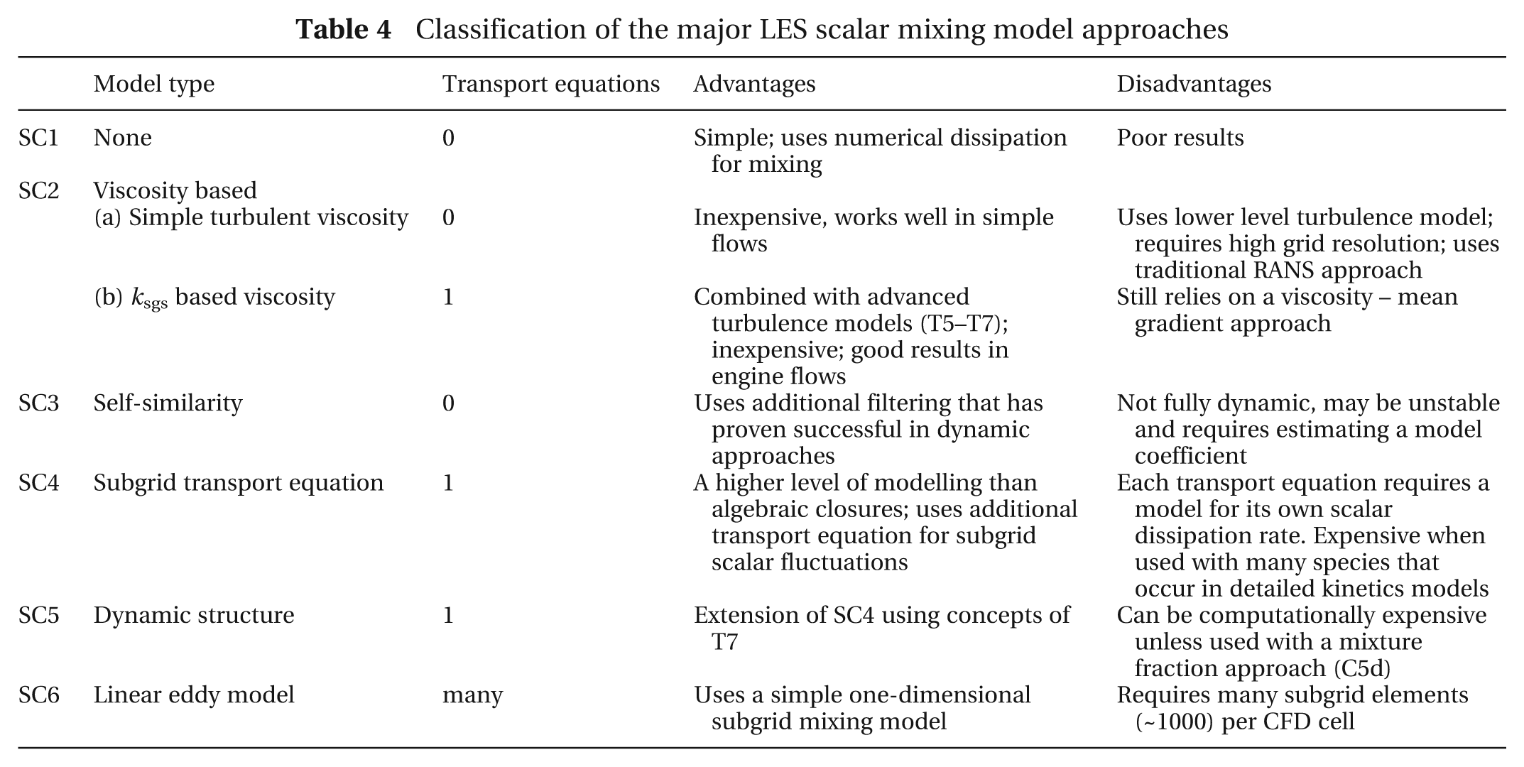
SC1. As with the T1 turbulence model, one can rely on numerical dissipation to provide mixing [20]. This does not work well for reacting flows and is rarely used even for passive mixing.
SC2a. The viscosity and mean-gradient approach is essentially the traditional RANS model with the turbulent viscosity provided by the LES model (see equations (7) or (8)). As in RANS modelling, LES turbulent viscosity is combined with a turbulent Schmidt or Prandtl number. These numbers may be assumed constant or evaluated through dynamic procedures (see, for example, Moin et al. [123]). Probably, this is the most common scalar mixing model used in LES simulations, even for reacting flows [104]. The model relies heavily on the turbulence model.
SC2b. An important extension of the viscosity approach is to combine it with the one-equation turbulence models (T5–T7). In this case, the turbulent viscosity is formulated with the subgrid kinetic energy (equation (8)) and combined with a turbulent Schmidt or Prandtl number. This approach is used with LES in IC engine applications [15]. It provides good results at reasonable computational expense. This is primarily because it is combined with advanced turbulence models T5–T7.
SC3. Scale-similarity models are based on the same concepts that underlie many of the turbulence models (T3, T4, T6, T7, and appendix 3). Thus, this approach has the potential to be very accurate. This has been demonstrated by Moin and others [103, 123] from comparison with DNS results and for dump-combustor simulations. However, the approach does not appear to have been used for LES engine simulations yet. In addition, since scale-similarity models allow backscatter, which can result in unrealizable scalar values, SC3 models would require additional dissipation.
SC4. The transport equation model approach uses a traditional transport equation for the subgrid scalar flux or the subgrid scalar fluctuations. This is a logical evolution of LES scalar models (see Jiménez et al. [19] for discussion), but has only been used in LES modelling in the context of the dynamic structure approach (SC5). Probably the primary reason this approach has not been used is that every scalar (e.g. species and energy) requires an additional transport equation, and this can become very expensive. This is true, especially if simple turbulence models are used and high grid resolution is required. In addition, each transport equation requires a model for the subgrid scalar dissipation. This approach could be used in C4 type combustion models, especially the mixture fraction models where the only scalar transport required is for the mixture fraction variable.
SC5. The dynamic structure approach of T7 was extended for scalar transport modelling by Chumakov and Rutland [124]. This involves a transport equation for the subgrid scalar fluctuations that is then used with the dynamic structure approach to model the scalar flux. This can work well, but can be expensive because, just as with SC4, an additional transport equation for the fluctuating component of each species is required. Chumakov is continuing work on similar advanced scalar flux modelling for LES, and the results look promising [125]. However, testing on engine applications is still required.
SC6. The linear eddy model (LEM) approach uses a very different concept to model subgrid scalar mixing. In LEM, a one-dimensional (1D) unsteady equation, which can contain mixing, diffusion, and reaction is solved in each CFD computational grid cell. The emphasis of the LEM approach is on the mixing term that is modelled using a triplet mapping. This is a simple rearrangement of values based on length and time scales that mimic turbulent eddies. The original concept was developed by Kerstein [126] for turbulence. However, it is Menon’s group that has carried out a lot of work extending LEM for reacting flows [39, 60]. This approach can be expensive because a large number of grid points are used within each CFD grid cell for the 1D equations. Partly from the increased CPU resources and improved algorithms, the approach gives nice results [38, 127, 128]. The LEM can be parallelized, but it is not practical for applications at this time and has not been used in engine LES.
3.3.1 Scalars: additional considerations
Scalar dissipation rate. A scalar dissipation rate term can arise in several different ways when modelling scalars and combustion. As noted in the previous section, it may be used as a time scale in combustion modelling. For scalars, it often occurs in prescribed PDF combustion models, in which a mean and variance of some scalar is required. Commonly, the scalar is the mixture fraction, and transport equations for both the mean and variance are used. Within the transport equation for the variance, the scalar dissipation rate occurs.
The most common approach for scalar dissipation rate modelling in LES is one that is based on RANS modelling and uses the turbulence time scale [19]. However, this does not make sufficient use of LES concepts, and has been shown to give poor results in a priori engine studies [63]. More promising approaches based on scale-similarity ideas have been developed by Chumakov [129] for general flows and by Zhang et al. [63] for engine LES.
Scalar variance. Another approach to modelling the scalar variance is to avoid using a transport equation and use an algebraic closure. This approach has been developed for use in LES using scale-similarity concepts by Cook and Riley [130], Cook [131], and Jiménez et al. [19]. This avoids the need for a scalar dissipation rate model in the transport equation. In addition, the approach seems to provide a sufficiently accurate mixture fraction scalar variance for use in C4d prescribed PDF combustion models. The approach has been used in LES diesel engine modelling as part of a multimode combustion model, and gives good results when compared to experimental data [44]. However, there is strong evidence from Colin and Benkenida [132] that an algebraic closure is insufficient in flows with sprays, indicating that additional research is needed.
3.3.2 Scalar mixing: recommendations
Scalar mixing and combustion models are often linked through terms such as the scalar dissipation rate. This requires that the scalar models at least be consistent with the combustion model being used.
One major trend is to include detailed chemistry effects by direct integration or tabulation methods. This means that a large number of scalar transport equations are being solved. Thus, scalar mixing models should be fairly simple to avoid large computational costs.
Scalar mixing models that use a turbulent viscosity and mean scalar gradient (SC2) can be sufficient, provided they are coupled with advanced turbulence models (T5–T7) that provide additional subgrid variables such as Ksgs.
Higher order scalar mixing models that use transport equations for subgrid quantities (SC4, SC5) may offer better potential for accuracy but at a higher computational cost.
3.4 Fuel-spray modelling
Most engine simulations use the Lagrangian spray parcel methodology originally developed for RANS approaches in which the CFD grid is not resolved around spray particles. This approach was initially developed by O’Rouke and Amsden in the KIVA-II code, and this still provides the basis of most engine spray CFD modelling [133]. In this context, the spray modelling issue is how to represent the subgrid interaction of the Lagrangian spray particles with the continuous gas phase. This interaction includes momentum transfer (e.g. drag), kinetic energy transfer, heat and mass transfer during evaporation, and models for atomization, breakup, and collisions. This is an extensive list of complex physical processes, and they all require modelling. The range of physical processes and their complexity is probably why most spray models in LES are extensions of RANS approaches and little work has been carried out on developing new spray models specifically for LES applications.
A review of more general spray modelling was provided by Jiang et al. [134]. They discussed basic issues of using the parcel approach for RANS and LES. Most simulations of engines with sprays have used existing RANS spray models with simple modifications for use with LES turbulence models. In a series of papers, Bellan et al. have carried out extensive work exploring particle-based spray models for both DNS and LES simulations [135–139]. This is more fundamental work, but the target applications are those that use the Lagrangian parcel approach. Some of their major conclusions are listed below.
A good LES turbulence model is essential because the spray is affected by both the large-scale flow features as well as the subgrid effects. Both require a good turbulence model.
Viscosity turbulence models (T2–T6) can work with spray models, as shown by comparisons with DNS results. However, in an actual LES simulation, additional dissipation is needed. In general, spray models that work well in comparison to DNS results often are not sufficient for use in a stand-alone LES simulation.
The subgrid turbulence and scalar mixing models should consider anisotropy and inhomogeneities. This is because the length scale of the spray parcels is so much smaller than the grid scale that these differences can be important.
The number of parcels that is appropriate for use in the LES spray models is not well understood.
There must be full interaction between the spray and the gas phase. This means that partial models that only include gas flow affects on the spray but ignore spray effects on the gas flow are not sufficient.
The Lagrangian spray parcels are not located at the grid points. Thus, obtaining accurate values of the gas phase variables (velocity, temperature, concentration) at the spray parcel location is important. A simple interpolation is not sufficient, and Bellan et al. found that a random perturbation from a normal distribution is required. For drag effects, this is similar to including turbulent dispersion effects commonly used in RANS spray models.
This is a rigorous list to keep in mind as spray models are developed and evolved for LES engine simulations. A list of the spray modelling approaches that could be used in engine LES applications appears in Table 5.
Classification of LES spray modelling approaches
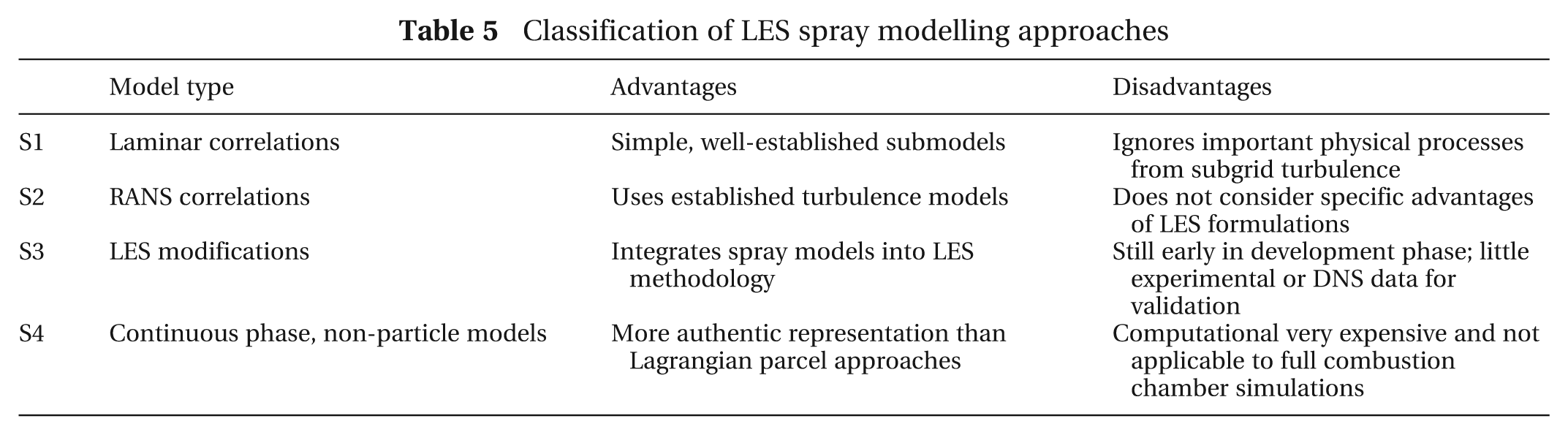
S1. The simplest approach to LES spray models is to use laminar correlations for subgrid interactions such as drag and evaporation. This means obtaining droplet drag, heat transfer, and mass transfer effects on both the gas and liquid phases through correlations appropriate for laminar flow around drops. This approach might be acceptable for very high resolution, scientific LES. However, it is inappropriate for engineering LES since there are subgrid turbulence effects that are important and need to be modelled.
S2. The use of RANS correlations is probably the most commonly used approach for spray modelling in LES. Here, subgrid models based on single droplet turbulent correlations for drag, turbulent dispersion, evaporation, and even breakup and collision are used with LES turbulence models. Successful examples of this approach for engines can be found in: (a) Hu et al. [15] and Hu and Rutland [78] for diesel applications with the T7 turbulence model and a multimode combustion model, (b) Kaario et al. and Vuorinen et al. at Helsinki University of Technology [10, 140] for diesel applications with T5 and later T1 turbulence models and a C3a combustion model, and (c) Aria et al. [141] for direct injection gasoline applications using a T2 turbulence model.
In a series of papers, a group at Doshisha University has explored spray models using KIVA with the T5 turbulence model [52, 53, 142–144]. The spray models were essentially the same as the RANS-based models available in the original KIVA code. Their work focused on non-engine simulations of spray bombs with fairly dense grids. They made nice comparisons with experimental work, demonstrating that the S2 approach for spray modelling can provide reasonable results with very high grid resolution. One interesting aspect of their work was the addition of a higher order numerical method for momentum equation convection terms. Their results demonstrated moderate improvement with the new numerical technique. However, it was achieved only on a simple Cartesian grid used in their spray bomb domain and might be difficult to achieve on a practical engine grid.
S3. The most desirable spray models would be those that are developed specifically for LES and are fully consistent with the turbulence and scalar mixing models. These would take advantage of the information from the LES models such as subgrid turbulence, ksgs, for modelling the many fuel-spray processes. There was some initial work on this carried out by Pannala et al. [145]. They made an important observation that models should consider that the interaction between the spray and the gas flow occurs at both the subgrid and the resolved scales. They developed a partitioning to account for this but, unfortunately, the work was not well explained so it is hard to evaluate.
More recently, Bharadwaj et al. developed an LES specific model for diesel sprays [146, 147]. The model reformulated the spray source term in the subgrid kinetic energy transport equation of a T7 turbulence model. The model used a deconvolution method [148] to obtain a better representation of subgrid velocities at the droplet location. The model addressed one of the primary problems with using RANS spray models with LES turbulence models. In these situations, it is not uncommon to see high-speed sprays significantly over-penetrating unless a very dense grid is used [142]. This can be traced to the RANS spray source term being modelled only as a sink of kinetic energy, whereas in the LES formulation, the spray can be either a source or a sink depending on the spray velocities and the ambient gas conditions. Figure 5 demonstrates how an LES simulation without an appropriate source term has significant over-penetration of the liquid parcels while the addition of the source term from Bharadwaj et al. brings the penetration in line with the experimentally calibrated RANS results.
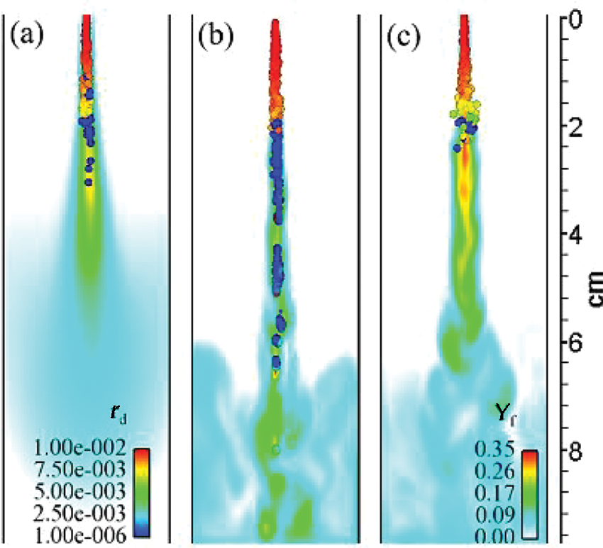
Droplet radius (rd(cm)) and vapour mass fraction (Yf) for 110 MPa injection pressure into a spray vessel with a density of 30.2 kg/m3: (a) RANS, (b) LES with no spray source model, and (c) LES with the spray source model [146]
S4. Recently, there have been a number of publications describing high-resolution, very detailed simulations of fuel sprays. In a paper by deVillers et al. [149], a volume of fluid (VOF) approach was used to study near-nozzle flow and primary breakup in a diesel spray. They used the OpenFOAM code [150, 151] with a T5 turbulence model on a very dense grid. The VOF method used was adapted for droplet breakup, but no other specific LES spray models were used. In later work, Befrui et al. [152] used the VOF method to simulate internal and near-nozzle flow for gasoline direct injection applications. They used the OpenFOAM code with a T5 turbulence model, a very dense grid and no special submodels for the spray. Similar work was carried out by Bianchi et al. [153] using a T2 turbulence model and the VOF method. Drozada and Oefelein [154] also used a very dense grid with an in-house code to simulate internal and near-nozzle high-pressure hydrogen gas injection.
These types of studies use very dense grids and are computationally very expensive. Thus, with current computer technology, they are not appropriate for practical engine applications. These simulations fall in the category of scientific LES, and are very useful in understanding more basic aspects of sprays and fuel injection. They will be very useful as baseline case studies for development and testing of S3-type spray models.
Another interesting recent approach is to combine an Eulerian description of the spray very near to the nozzle exit that transitions into a Lagrangian model further downstream. For example, Martinez et al. [155] used this type of model for LES of diesel injectors. The advantage is that the Eulerian description is better able to capture momentum flux and entrainment than a pure Lagrangian approach without requiring dense grids. The method shows promise, but it can be sensitive to the models used to transition from the Eulerian to the Lagrangian description, and additional work is needed.
3.4.1 Fuel spray: recommendations
The development of LES spray models is behind work on other LES models. In practice, it appears that using S2 spray models with calibrations to work with LES turbulence models may be adequate for the time being. However, this approach tends to have strong grid resolution dependencies. As more S3 models are developed specifically for LES, these should be better choices. As always, the higher order turbulence models (T4–T7) should be used, and simulation efforts should be strongly coordinated with experimental data for model calibration.
4 Examples of LES Engine Studies
In this section, several studies are described in which LES has been successfully used to study some aspect of IC engines. These help to demonstrate how LES is currently being used. Currently, one of the primary successful applications has been to study cycle-to-cycle variability, and several studies are described below. In addition, several research groups are using LES to study HCCI type diesel applications. For each of the cases described below, the types of models used are listed according to the nomenclature used in Tables 2–5.
Haworth et al. (T2) were one of the first to examine cycle-to-cycle variability, albeit in a motored engine [33, 34]. The simulations used a T2 turbulence model and were for a simple, very well instrumented engine known as the GM TCC engine [156, 157]. The engine has two valves and is a pancake, four-cycle single-cylinder configuration. Haworth’s group simulated several consecutive motored cycles and saw variations in swirl, tumble, and instantaneous flow structures.
The FEV Motorentechnik and RWTH in Aachen (T2, SC2a, and S2) have used LES to examine cycle-to-cycle variation of mixture preparation in a direct injection SI engine [158]. They used the commercial code STAR-CD and simulated ten different cycles through intake and compression to the point of spark ignition. Since they did not simulate combustion and the exhaust process, the simulations were not for consecutive cycles. Instead, the Aachen groups used intake port pressure measurements as boundary conditions for the simulations. This creative approach allowed them to look at some aspects of cyclic variation of mixture preparation without the complications of modelling combustion. The group found very good agreement between PIV and LIF images and the simulation results for chosen flow cycles. They also carried out statistical analysis and found a reasonable comparison with experimental results for the probability of misfire due to a lean mixture at the spark location.
More recently, the Aachen group used LES to study high-speed diesel engines. Adoph et al. [159] used single-cycle LES to study the impact of port design on emissions. The study combined PIV measurements and LES to evaluate the impact of port design on in-cylinder flow mixing and homogeneity. These were then correlated with engine out emissions data from a single-cylinder test engine over a range of EGR levels. This work was continued by Rezaei et al. [160] using PIV, RANS, and LES to evaluate swirl homogeneity from different intake valve lift strategies. In this study, multiple cycles were used, and the effects of pressure variations at the intake port boundary condition were included.
As noted in previous sections, several groups in France (IFP and CERFACS (T2, C4c, and SC2a)) have been working to develop LES for engines using a code adapted from CERFACS. In several recent publications, they demonstrated nice work on using LES to study cyclic variation in a port fuel injected SI engine [59, 161]. In this work, the simulations were for nine to ten consecutive cycles that include combustion. The engine operating condition studied used propane fuel with a 0.7 equivalence ratio. Both the experimental data and the simulations showed a very high degree of cycle-to-cycle variation (up to 25 per cent variation in peak pressure). The ten LES simulation cylinder pressure traces were within the envelope of the experimental data. The simulations used a very high grid resolution, 250 000 to 628 000 cells, and resulted in detailed images of the in-cylinder flow as shown in Fig. 6. From these types of results, the cyclic variation was attributed to differences in intake turbulence that resulted in quantitative changes to combustion and flame propagation.
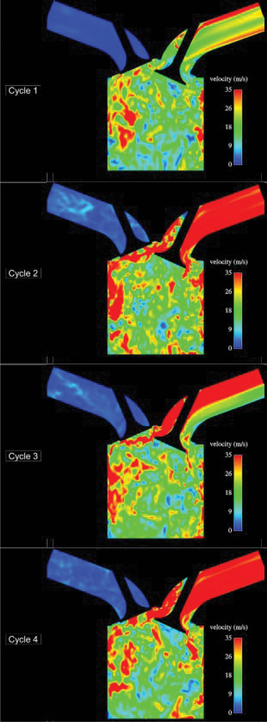
Cyclic variation demonstrated by velocity magnitudes in a centre cut-plane of a PFI engine at 235°CA BTDC (from [161], reprinted with permission from SAE paper 2007-01-0151, © 2007, SAE International)
The research group at Lund University (T3, C4a, and SC2a) has been using LES with experiments to study HCCI combustion with diesel fuel. In a series of papers, the impact of chamber geometry, turbulence, initial temperatures, and wall temperatures on HCCI has been studied [31, 83, 84, 162, 163]. The simulations were used effectively to understand and explain the impact of these processes on HCCI combustion. Very high grid densities of over two million cells were used, which used to be common for DNS isotropic turbulence studies. Also, a progress variable combustion model (C4a), rather than a purely kinetics-based model (C1), which is more common for capturing HCCI ignition, was used.
The group at the Engine Research Center (T7, mixed mode: C1–C3b–C4d, SC2b, and S3) has been developing LES for diesel engine applications for several years [40, 41, 43, 78, 164]. This work was focused on addressing the major modelling requirements in engine CFD and adapting the models specifically for LES. This included work on the turbulence model, the combustion model, and the spray models. The results were engine simulations that compared well with experimental results. In addition, when applied to HCCI combustion, the simulation results were able to capture cyclic variability due to temperature non-homogeneities in the spray region.
5 Prospects for the Future
The outlook for using LES in IC engine modelling is very good. The primary engine submodels, as outlined in this review, are maturing. User experience is growing, and the number of high-quality studies using LES is rapidly increasing.
There is still a need for model improvements, especially in the areas of combustion and sprays. However, this need is not unique to LES. In addition, improvements and adaptation to LES are needed for many second-tier models such as wall heat transfer, nozzle flows for spray boundary conditions, spray breakup, and atomization.
Improvements to numerical methods are also needed. However, improvements will be somewhat limited by the complexity of the domain, moving boundaries, and numerical treatment of fuel sprays. These limitations should not preclude the use of LES in engines, as there is still much to be gained in terms of increasing the types of problems that can be studied.
Important issues that remain on the horizon are validation and establishing ‘best practices’ for LES engine simulations. Increasing activity and publications will help to address these issues naturally. In addition, there is a high probability that research groups are already establishing programs to address these issues as the potential of LES becomes clearer.
Thus, users are encouraged to apply LES to appropriate problems that are enhanced or require the increased sensitivity to flow unsteadiness and large-scale structures. For example, topics such as cyclic variation and design sensitivity are probably best studied with LES. However, users should be aware of the large range of models used in engine CFD and carefully choose the appropriate LES capable submodels. The taxonomy presented in this review should be helpful in this regard.
Footnotes
Appendix 1
Appendix 2
Appendix 3
Appendix 4
The author acknowledges support over the years in the broad area of LES for engineering applications from a number of sources, including the US Department of Energy [grant numbers DE-FC04-02AL67612, DE-FC26-06NT42628, and DE-EE000 0202], General Motors Research primarily through the GM-UW Cooperative Research Lab, Caterpillar Inc., the National Science Foundation [grant number 0500056], and the Air Force Office of Scientific Research [grant number F49620-02-1-0348].