
Abstract
This article examines how caste shapes access to credit in India’s formal and informal lending markets. Using nationally representative data from the India Human Development Survey (2011–2012), we analyse loan application rates and loan amounts and compare outcomes between General Castes (GC) and three lower-caste groups: Other Backward Castes (OBC), Scheduled Castes (SC) and Scheduled Tribes (ST). We find that GC households are more likely to apply for and receive larger loans from formal banks, while lower-caste households rely more heavily on informal moneylenders. A substantial share of these credit gaps—particularly in bank lending—remains unexplained by observable characteristics, pointing to potential caste-based discrimination. In contrast, moneylenders do not appear to penalize lower-caste borrowers to the same extent and, in some cases, lend more than expected to OBC households. These findings suggest that entrenched caste hierarchies continue to influence credit access in India, with formal institutions reinforcing rather than correcting social inequalities.
I. Introduction
India’s caste system represents one of the world’s most enduring forms of social stratification, profoundly shaping economic opportunities and social mobility for over a billion people. Despite constitutional abolition of caste-based discrimination in 1950, this ancient hierarchy continues to influence virtually every aspect of Indian society—from education and employment to housing and financial services (Deshpande, 2000; Kijima, 2006; Thorat and Attewell, 2007). The rigid social hierarchy traditionally assigned occupations, resources and rights along hereditary lines, with upper-caste groups controlling most resources and well-paying occupations, while lower-caste communities were relegated to menial and low-paying work (Mosse, 2018). Although the most overt practices of untouchability and public discrimination have been outlawed, caste-based divisions persist in more subtle but equally consequential forms across economic, social and political spheres.
Credit access represents a fundamental pathway through which caste continues to influence economic outcomes in contemporary India (Thorat, 2009). Access to financial resources is widely acknowledged as critical for facilitating upward economic and social mobility, enabling entrepreneurship, agricultural investment and poverty reduction (Duflo and Banerjee, 2011; Kaboski and Townsend, 2012). Conversely, systematic exclusion from credit markets can perpetuate intergenerational cycles of disadvantage, particularly for historically marginalized communities.
The importance of credit access cannot be overstated in the Indian context. Credit serves as one of the most critical constraints to economic advancement for lower castes (Thorat, 2009), with variations in access constituting a major source of income inequality (Demirgüç-Kunt and Levine, 2009). Previous research has demonstrated that lack of credit access constrains entrepreneurship (Banerjee et al., 2017), limits agricultural investment and farm production (Kochar, 1997), restricts spending on education (Doan et al., 2014) and impedes poverty reduction efforts (Chowdhury et al., 2005). These constraints are particularly acute for lower-caste groups who remain socially excluded from mainstream economic opportunities and lack access to assets, public facilities and networks that could improve their economic prospects (Thorat and Neuman, 2012).
Credit access can be shaped by caste through multiple mechanisms. A lower-caste loan applicant may face discrimination from bank officials or moneylenders not just in terms of approval but also regarding loan amounts. This discrimination may be entirely driven by caste prejudice—what Becker (2010) defines as ‘taste-based discrimination’. Alternatively, lenders may believe certain caste groups represent higher default risks, leading to statistical discrimination as conceptualized by Arrow (1973) and Phelps (1972). Complicating matters further, anticipating such discrimination, lower-caste borrowers may apply for smaller loans or may not apply at all, creating a self-fulfilling prophecy where fear of discrimination reduces credit demand.
A growing body of research has explored the relationship between caste and credit in India, though with varying methodological approaches and findings. Kadam et al. (2024) investigated small business credit access and found that entrepreneurs from marginalized castes receive significantly lower loan amounts. Patel et al. (2022) examined caste discrimination in microfinance loan approvals, finding that females from a lower caste, relative to those from a higher caste, have lower odds of receiving loans. Kumar and Venkatachalam (2019) examined caste-based discrimination in agricultural credit, finding marginalized caste borrowers are less likely to apply for bank loans. Khanna and Majumdar (2020) found that some lower castes pay substantially higher interest rates and get smaller loans in the informal lending sector.
In this article, we examine whether a borrower’s caste influences their access to credit. We focus on two key dimensions: the probability of applying for a loan and the amount borrowed. Our analysis uses data from the India Human Development Survey (IHDS), conducted in 2011–2012, which covers over 41,000 households. The data give information on households credit outcomes as well as their caste identity, along with an array of other information. We look at four broad caste categories—a grouping of higher caste, which we call General Castes (GC), and three groupings of lower castes, namely Other Backward Castes (OBC), Scheduled Caste (SC) and Scheduled Tribes (ST). The social hierarchy places OBC ahead of SC and ST.
Our empirical strategy compares GC with each of the three lower-caste groups across two types of lenders: formal banks and informal moneylenders. For each, we analyse differences in loan application rates and loan amounts. We use the Blinder–Oaxaca decomposition technique to separate the observed gaps into portions explained by differences in household characteristics (such as income, land, education and occupation) and those that remain unexplained. The unexplained component, while not conclusive proof of discrimination, could reflect omitted variables correlated with caste (Deshpande and Sharma, 2014). This is a limitation common to all decomposition analyses. To address potential endogeneity in current income, we instrument household income using past income reported in the 2004–2005 wave of IHDS.
We find four main results. First, GC households are more likely to apply for bank loans, while lower-caste households are more inclined to seek credit from moneylenders. Second, GC borrowers receive larger loan amounts from both banks and moneylenders, even though lower-caste households rely more heavily on informal credit. Third, a substantial part of these credit gaps remains unexplained by observable characteristics, suggesting the presence of discrimination or systematic bias in formal lending. Fourth, moneylenders do not disadvantage lower castes to the same degree; in some cases, they even appear to favour OBC borrowers beyond what their observable characteristics would predict.
These findings highlight how caste shapes not only who participates in different segments of the credit market but also how borrowers are treated once they apply. In formal banking, strict rules, paperwork and risk models tend to favour GC households, while lower-caste borrowers may be judged as riskier or discouraged from applying at all. In contrast, moneylenders rely more on local knowledge, relationships and social pressure to ensure repayment. This makes them more willing to lend to lower-caste borrowers and in some cases even prefer them, because repayments can be enforced informally. Together, these findings show that differences in how lenders assess and enforce risk help explain why credit gaps between castes look different in banks compared to moneylenders.
This study makes several important contributions to the existing literature on caste-based credit discrimination in India. First, most studies focus on either formal or informal credit markets but rarely compare discrimination patterns across both sectors systematically. Second, we distinguish between productive and consumption loans, uncovering differential patterns of discrimination based on loan purpose. Third, unlike previous research, this analysis employs Oaxaca–Blinder decomposition to quantify the extent to which observed credit gaps can be attributed to differences in observable characteristics versus potential discrimination, while addressing selection and simultaneity bias.
This article is structured as follows: Section II presents data and uses descriptive evidence to highlight caste differences in India. Section III sets out the methodology for the article. Section IV presents and discusses the results. Section V concludes the article.
II. Data and Sample Characteristics
The data used in the article come from the IHDS—a nationally representative survey of 42,152 households in 2011–2012 collected from 1,503 villages and 971 urban neighbourhoods across India. The survey covers a range of questions relating to economic activity, income and consumption expenditure, assets, social capital, education, health and marriage. Additionally, we use household income data from the earlier round of the IHDS (2004–2005) to construct our instrumental variable.
Table 1 presents the descriptive statistics of the variables of the four caste groups used in the analysis. The proportion of caste groups used in IHDS 2011–2012 is similar to National Sample Survey (2006), where GC are 30%, OBC are 41.1%, ST are 8.6% and SC are 19.5%. GC households report the highest average loan amounts and the highest share of borrowing from formal banks. In contrast, OBC, SC and ST households rely more on informal sources, especially moneylenders. While 46% of GC households participate in the credit market, this share is higher for OBCs (60%) and SCs (56%), and slightly lower for STs (44%).
Summary Statistics.
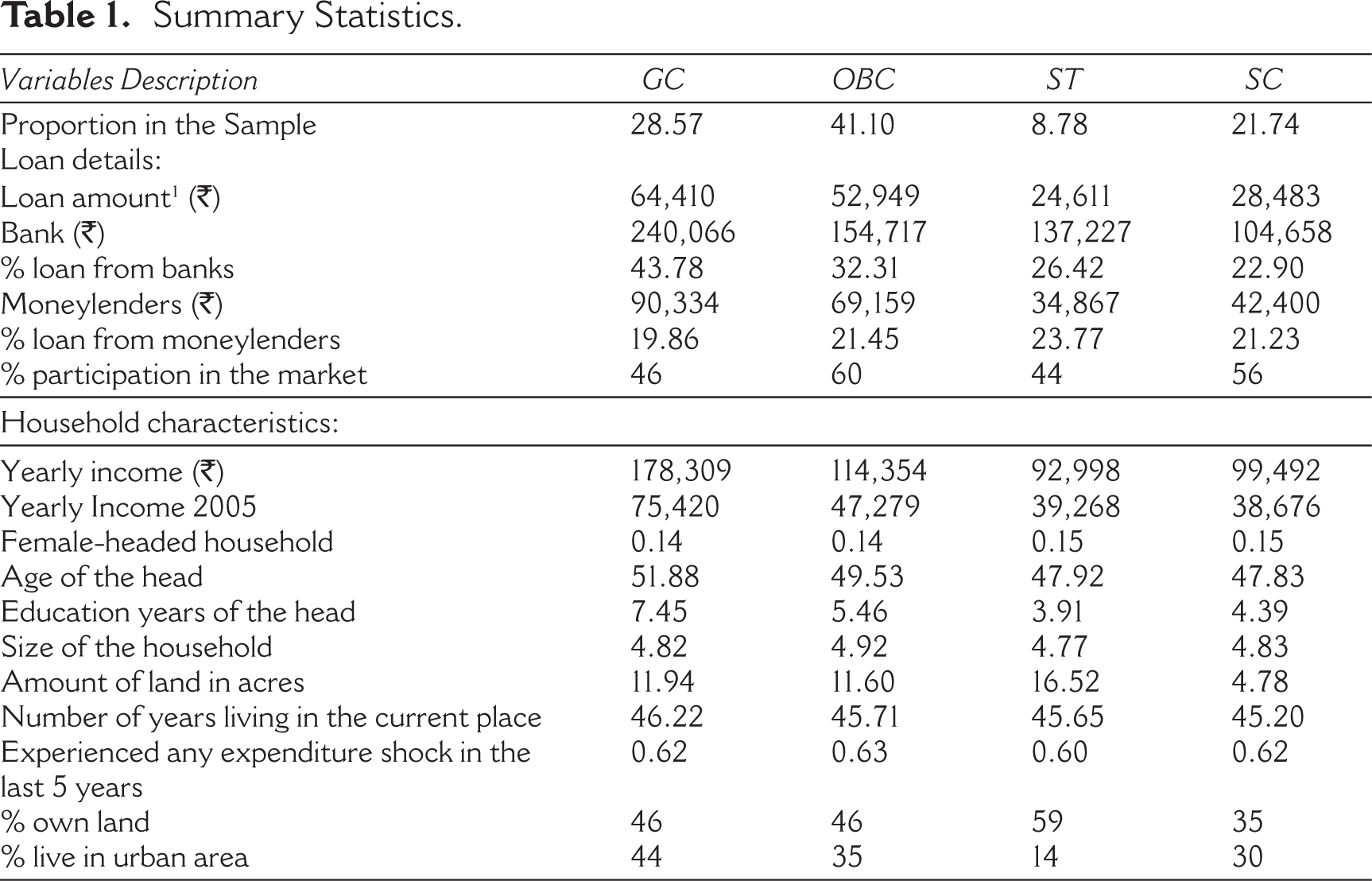
Caste-based stratification translates into low human capital for lower-caste individuals. The average number of education years completed by ST (head of the households) in the sample was 3.91 years, 4.39 years for SC, 5.46 years for OBC, followed by 7.45 years for the GC. Generally, the differences at lower levels of education (primary) are less pronounced across social groups but start to diverge widely by middle school and higher. For instance, only 3.5% of the SC heads of household have achieved a graduate or postgraduate education compared to 14% of GC individuals.
Substantial caste-based disparities are also evident in income, education and landholding. GC households report the highest average income (₹178,309), followed by OBCs (₹114,354), SCs (₹99,492) and STs (₹92,998). The average number of education years completed by ST (head of the households) in the sample was 3.91 years, 4.39 years for SC, 5.46 years for OBC, followed by 7.45 years for the GC. Generally, the differences at lower levels of education (primary) are less pronounced across social groups but start to diverge widely by middle school and higher. For instance, only 3.5% of the SC heads of household have achieved a graduate or postgraduate education compared to 14% of GC individuals. Although lower-caste households are more likely to live in rural areas, they often own less land: only 35% of SC households and 46% of OBC households report land ownership, compared to 46% among GCs and 59% among STs.
Other household characteristics such as age of the household head, household size and residential stability (years spent in the same location) show little variation across caste groups. Around 14%–15% of households are female-headed in all groups, and over 60% report having experienced an expenditure shock in the past five years due to illness, natural disaster, marriage, unemployment, death or crop failure—suggesting that economic vulnerability is common but not necessarily caste-specific.
III. Methodology
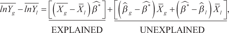
This article presents estimates of the credit differential between castes in the Indian credit sector and the extent to which this differential can be explained by differences in observable characteristics or ‘endowments’ of clients across caste groups. The amount of credit the borrower has arises from the following equation:

where lnY is the natural logarithm of the loan amount of ith individual in jth social group ranging from GC, SC, ST and OBC. Xij is a vector of observed characters, and βj is a coefficient vector to be estimated for each caste type, and uij is assumed to be a normally distributed error term.
The Blinder–Oaxaca decomposition is employed to decompose the credit amount gap in outcomes between various castes. 2 Oaxaca (1973) and Blinder (1973) introduced a regression-based decomposition method that separates the observed gap in an outcome between two groups into an ‘explained’ component and an ‘unexplained’ component. The explained component reflects differences in endowments and observable characteristics (such as education, income or assets) between the groups. The unexplained component, by contrast, captures differences in the returns to these characteristics—often interpreted as unequal treatment or structural bias. While the unexplained component is often used as a measure for discrimination in the literature (Amin et al., 2019), it is very likely that the residual also includes the effects of unobservable or unmeasurable characteristics. 3
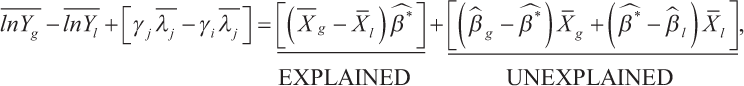
The difference in the credit amount arises from the following equation:
where lnY is the natural logarithm of the loan amount, g and l subscripts stand for general caste and lower castes (SC, ST and OBC), respectively. Xg is a vector of observed characters for the general caste, Xl is a vector of observed characters for various lower castes, and βg is a coefficient vector to be estimated for the general caste, β1 is a coefficient vector to be estimated for the lower caste and is the estimate of the non-discriminatory credit coefficient from a pooled regression over both groups (Neumark, 1988).
Selectivity and Simultaneity Bias
Another methodological problem faced in analysing the caste gap is the existence of endogeneity which can be caused by self-selection and simultaneity bias. Selection bias could occur when individuals with similar characteristics (education, assets or consumption level) have different levels of entrepreneurship, perseverance and ability, which may lead to different probabilities of their participating in the credit market. The Heckman two-step procedure (Heckman, 1979) corrects for sample selection bias by explicitly modelling two related processes: (a) the selection equation, which estimates the probability that a household chooses to apply for a loan, and (b) the outcome equation, which estimates the amount borrowed or the approval outcome, conditional on having applied. The method assumes the error terms in the selection and outcome equations are jointly normally distributed. The first step is typically estimated using a probit model that includes variables likely to affect the decision to seek credit, such as household composition, landownership, education and other relevant household characteristics. This yields an inverse Mills ratio (IMR), which summarizes the part of the error term correlated with selection. In the second step, this term is included as a regressor in the outcome equation to correct for selection bias. 4
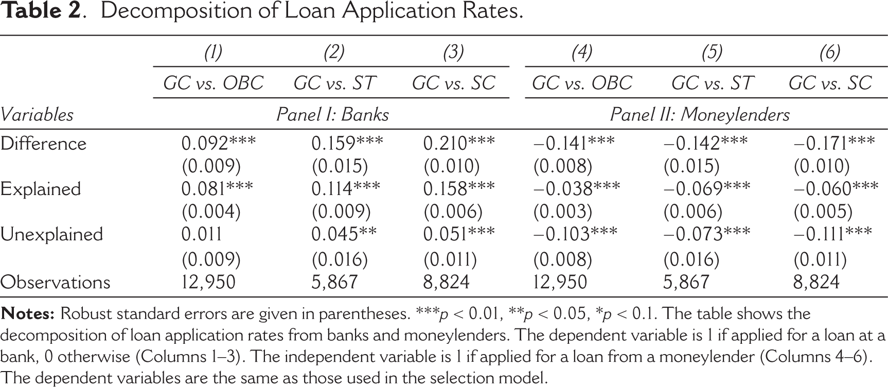
Using the Blinder–Oaxaca decomposition, the observed earnings differential can be further decomposed into:
where γ is the coefficient of the IMR (λ).
Simultaneity bias can arise due to the potential endogeneity of household income: Higher income may increase the amount a household borrows, while at the same time, obtaining larger loans could influence income (reverse causality). To address this, we require an instrumental variable (IV)— an exogenous variable that is correlated with current income (the endogenous regressor) but uncorrelated with the error term in the loan amount equation.
In this analysis, we use household income reported in 2004–2005 (from the first round of the India Human Development Survey, IHDS-I) as an instrument for current household income (measured in 2011–2012). Lagged variables are commonly used as instruments in the literature (Ackerberg et al., 2007; Doraszelski and Jaumandreu, 2018; Wang and Bellemare, 2019), leveraging temporal separation to address endogeneity.
The key identification assumption—the exclusion restriction—requires that past income affects current loan amount only through its effect on current income. Several factors support this assumption. First, the seven-year lag means lenders are highly unlikely to observe or consider historical income when making loan decisions; instead, they focus on current verifiable indicators such as employment, assets and recent earnings. Second, the major life-course traits that could channel past income into borrowing—such as household head’s education, land ownership and primary occupation—tend to be fixed over this period and are explicitly included as controls. As a result, any direct effect of past income on current borrowing should be negligible, except insofar as it operates through current income. 5
Past income is strongly correlated with current income in the first-stage regression (see Table A5) (satisfying the relevance condition) and F-statistics, providing further confidence in the instrument’s strength. The Cragg–Donald Wald F-statistic of 949.244 substantially exceeds the Stock–Yogo critical values for weak instrument bias, surpassing even the most stringent threshold of 16.38 for 10% maximal IV size distortion. This indicates that our instrument is sufficiently strong to avoid the bias and inference problems associated with weak instruments (Stock and Yogo, 2005). The Anderson canonical correlation LM statistic (903.661, p < .001) confirms that our equation is identified, rejecting the null hypothesis of under-identification.
IV. Results
Decomposing the Differences in Loan Application Rates from Banks and Moneylenders
We begin by estimating the probability of applying to either bank or moneylender. The dependent variable is 1 if the client has applied or 0 otherwise. The estimates of the probit regressions (see Tables A1 and A2 in the Appendix) are used to construct the IMR for the purpose of correcting the credit amount equation for selection bias as reported in the later section. Since participation in the credit market is a binary outcome, we cannot directly apply the standard Oaxaca–Blinder decomposition. Instead, we use Fairlie’s (2005) method, which adapts the decomposition approach for nonlinear outcomes.
Table 2 reports the decomposition of caste gaps in loan application rates into explained and unexplained parts, separately for formal banks (Columns 1–3) and informal moneylenders (Columns 4–6). The analysis compares GC with three other caste groups. The first panel shows participation gaps in bank credit. GC households are significantly more likely to apply for bank loans than all three disadvantaged groups. The loan application rate difference ranges from 9.2% points between GC and OBC, 15.9% points between GC and ST and 21% points between GC and SC, all significant at the 1% level. The results suggest that most of these gaps are explained by differences in observable characteristics—such as higher education, greater land ownership and higher income among GC households. For example, in the GC versus SC comparison, 15.8% points of the 21-point gap is explained by these characteristics. The remaining unexplained component—which may reflect discrimination, anticipatory exclusion or unobserved traits—is small but statistically significant in some cases: 5.1% points for GC versus SC and 4.5 points for GC versus ST. For GC versus OBC, the unexplained component is small and not significant, suggesting that most of the gap is driven by observable characteristics.
Decomposition of Loan Application Rates.
This pattern is consistent with the institutional features of formal banking: paperwork requirements, collateral demands and documented income history advantage households with higher socio-economic status—traits more common among GC households.
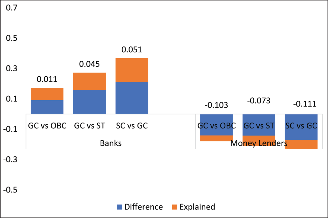
The second panel shows contrasting patterns for the loan application rate in borrowing from moneylenders. Here, lower-caste households are significantly more likely than GC households to apply for loans, as suggested by the negative coefficient. The loan application rate difference ranges from −14.1% points between GC and OBC, −14.2% points between GC and ST and −17.1% points between GC and SC. Part of this difference is explained by observed characteristics, but a substantial share remains unexplained and statistically significant, for instance, 11.1% points for GC versus SC, 10.3 for GC versus OBC and 7.3 for GC versus ST, suggesting that moneylenders lend to these groups at higher rates than observable traits alone would predict. Figure 1 visualises these caste differences in loan application rates, breaking down the explained and unexplained components for both banks and informal lenders.
Loan Application Rate Differences Between Castes in Lending from Banks and Moneylenders.
Several mechanisms could explain this. First, moneylenders operate in local markets where they have better information about borrowers’ true financial status, reputation and repayment history, reducing informational asymmetry. Second, moneylenders often rely on social and community-based enforcement, making it easier to extract repayment from households who are locally embedded and less legally protected. This aligns with the idea that marginalized borrowers may be seen as easier to discipline informally or, as Kuran and Rubin (2018) argue, more ‘financially powerless’—paradoxically increasing their attractiveness to lenders.
Overall, the results highlight a dual pattern: GC households are better positioned to access formal credit markets, largely because of favourable socio-economic characteristics, while lower-caste households disproportionately rely on informal lenders, partly due to structural disadvantage and partly because moneylenders may be more willing to engage with them beyond due to social networks and better information about their financial status.
Decomposing Credit Differential with the Selection Effect
Loan Amount
In the next stage, we examine caste differences in the loan amount taken from banks separately for production and consumption loans. To account for self-selection into borrowing and the potential endogeneity of income, we estimate Heckman two-step models with instrumental variables, as described in the methodology section (see Tables A3 and A4 in the Appendix). We then apply Blinder–Oaxaca decomposition to the loan amounts to disentangle how much of the caste gap is explained by observed characteristics (such as income, land and education) and how much remains unexplained.
Table 3 presents these results, comparing GC households with OBC, ST and SC households, separately for production loans (Columns 1–3) and consumption loans (Columns 4–6).
Credit Differences Between Castes in Bank Lending.
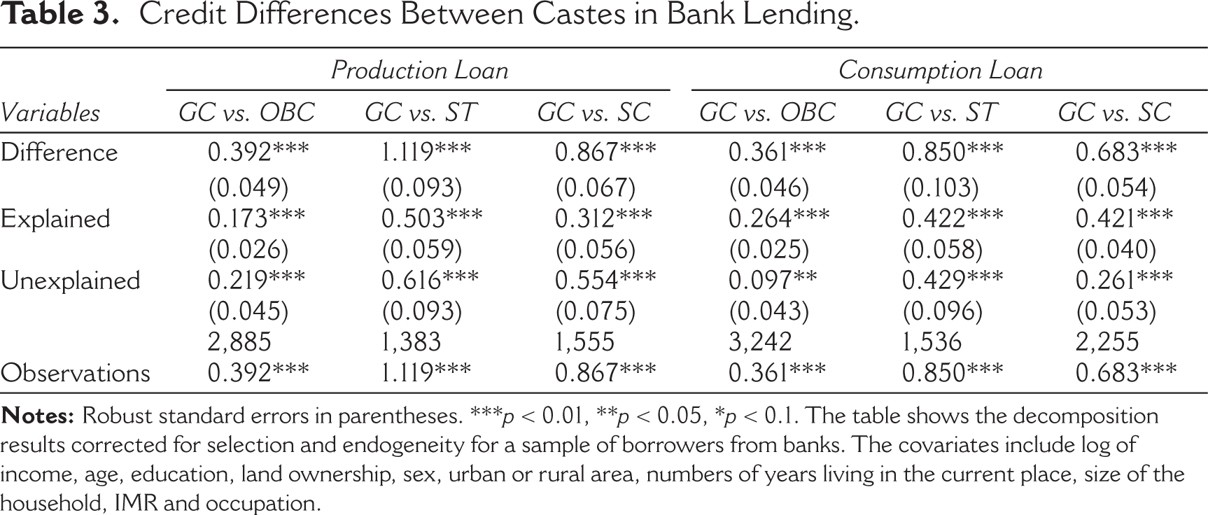
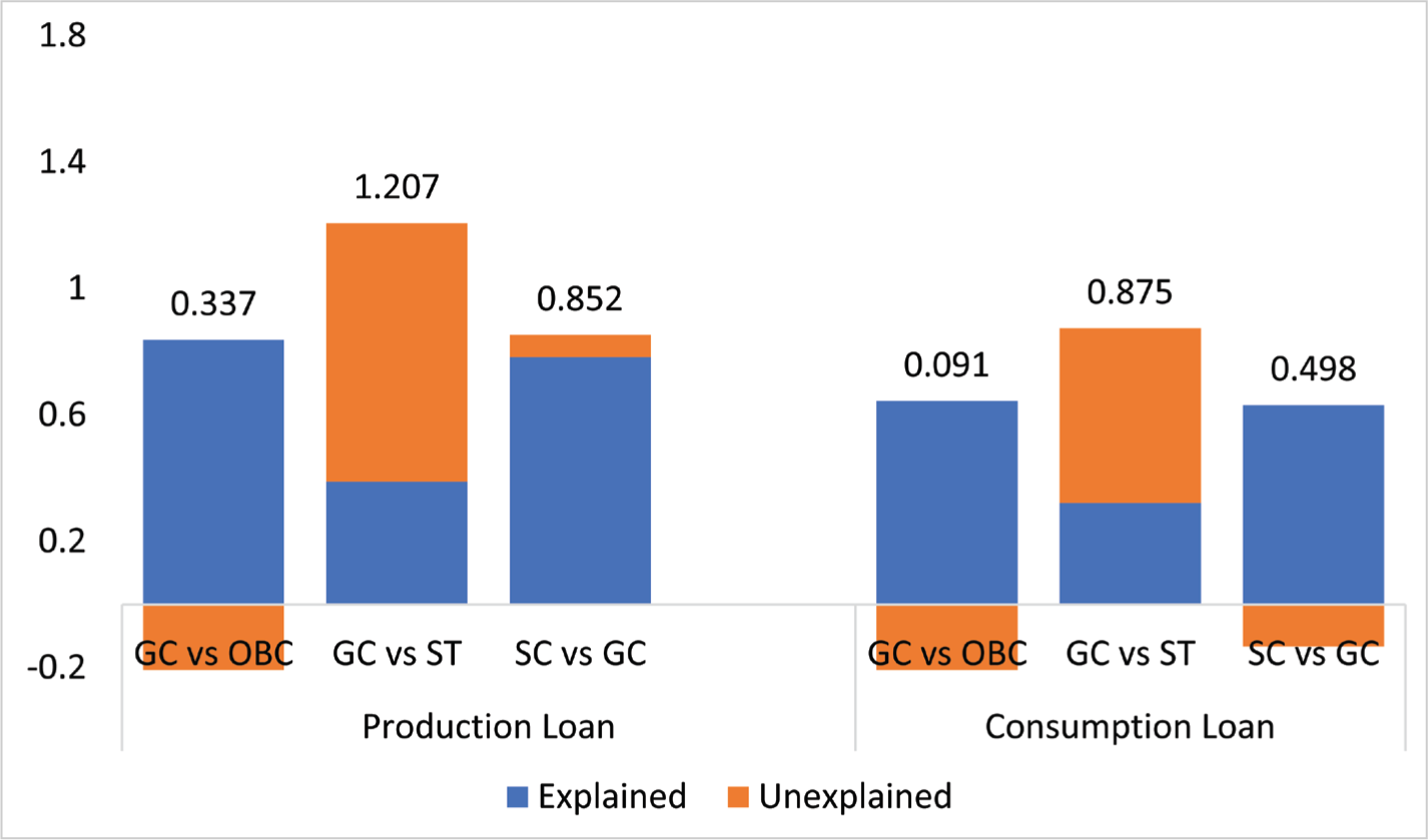
The adjusted credit differential shows that GC has an advantage of 0.39 log points (~48%) over OBC, 1.12 log points (~207%) over ST and 0.87 log points (~139%) over SC for production loans. A substantial portion of these credit differentials remains unexplained: 0.21 log points (~24%) between GC and OBC, 0.61 log points (~85%) between GC and ST, and 0.55 log points (~73%) between GC and SC. This unexplained portion suggests that even after controlling for measurable economic advantages, GC households still receive significantly higher loan amounts, possibly reflecting differential treatment by banks, unobserved creditworthiness or potential discrimination in loan allocation.
A similar pattern emerges for consumption loans. GC households again have a higher loan amount, with differences of 0.36 log points (~43%) for GC versus OBC, 0.85 log points (~134%) for GC versus ST, and 0.68 log points (~97%) for GC versus SC. Here too, part of the gap is explained by observable characteristics, but a sizeable unexplained component remains: 0.43 log points (~54%) for GC versus ST and 0.26 log points (~30%) for GC versus SC. Notably, the unexplained portion for GC versus OBC is smaller (0.097 log points or ~10%) but still statistically significant. Figure 2 provides a graphical summary of caste-based credit gaps in bank lending for both production and consumption loans, decomposed into explained and unexplained components.
Credit Differences Between Castes in Bank Lending for Production and Consumption Loans.
These findings imply that banks lend larger amounts to GC households not solely because they are objectively ‘better risks’ (e.g., higher income or collateral), but also due to factors that are not fully captured by observable characteristics. Possible mechanisms include implicit biases by loan officers, institutional norms that favour traditionally privileged groups or greater confidence in GC borrowers’ repayment capacity based on historical patterns.
Moneylenders
Although the share of moneylenders has reduced significantly over the past few years, they still play a major role in financing lower-caste borrowers. However, Table 4 shows that there are large credit differentials between the general caste and other lower castes.
Credit Differences Between Castes in Lending from Moneylenders.
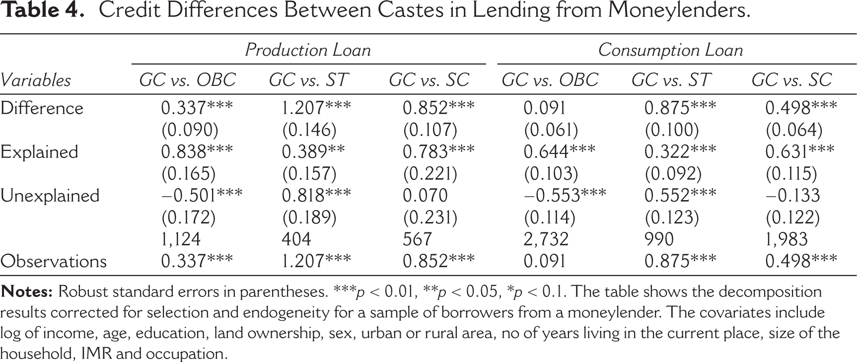
The adjusted credit differential, focusing on production loans obtained from moneylenders, indicates that GC households borrow significantly larger amounts than lower-caste households: 0.34 log points (~40%) more than OBC, 1.21 log points (~235%) more than ST, and 0.85 log points (~134%) more than SC.
For GC versus OBC, the explained component (0.84 log points or ~132%) is larger than the observed gap (0.34 log points or ~40%), while the unexplained component is negative and significant (−0.50 log points or approximately −39%). This means that based solely on observable traits like income, assets and education, GC households should borrow substantially more. Instead, moneylenders lend relatively larger amounts to OBC borrowers than their characteristics alone would predict, suggesting informal lenders may actually favour OBC borrowers or at least do not penalize them as formal lenders might.
For GC versus ST, both the explained (0.39 log points or ~48%) and unexplained (0.82 log points or ~127%) components are positive and significant, suggesting moneylenders lend more to GC borrowers partly due to better economic characteristics and partly due to unobserved factors or discriminatory preferences.
For GC versus SC, the unexplained component is small (0.07 log points or ~7%) and not statistically significant, indicating the gap is primarily driven by observable differences in characteristics.
In the case of consumption loans, the overall gaps are smaller: GC households borrow only 0.09 log points (~9%) more than OBC households (not significant), but substantially larger amounts compared to ST (0.88 log points or ~141%) and SC (0.50 log points or ~65%).
Again, the unexplained components vary. For GC versus OBC, the unexplained part is large, negative and significant (−0.55 log points or about −42%), implying that moneylenders extend larger loans to OBC households than their observable characteristics predict. For GC versus ST, the unexplained component is positive and significant (0.55 log points or ~73%), indicating possible unobserved favouring of GC borrowers. For GC versus SC, the unexplained component is negative (−0.13 log points or approximately −12%) but not significant, suggesting this gap can largely be explained by observable household characteristics. Figure 3 provides a graphical summary of caste-based credit gaps in informal lending for both production and consumption loans, decomposed into explained and unexplained components.
These patterns suggest that, unlike banks, moneylenders do not systematically favour GC borrowers. In fact, for OBC households, moneylenders lend larger amounts than observables would predict—reflected in negative unexplained components. The absence of a significant unexplained component for SC also suggests that the moneylender does not discriminate against SC. Several mechanisms might explain this. First, moneylenders often know their borrowers personally, which reduces perceived risk beyond what formal indicators capture. Second, marginalized borrowers may be easier to pressure or discipline if they default, making them attractive clients despite weaker formal profiles. As argued by Kuran and Rubin (2018), the legally privileged (like GC borrowers) may be harder to discipline, making lower-caste borrowers paradoxically more attractive from a risk-management perspective.
Credit Differences Between Castes in Lending from Moneylenders for Production and Consumption Loans.
Discussion of the Results
The results show that GC households obtain larger loans than lower-caste households across banks and moneylenders, for both production and consumption loans (with the exception of OBCs in one model, where the gap is positive but statistically insignificant). The critical difference lies not in the credit differentials but in the unexplained component of these gaps, which suggests how lenders treat caste groups beyond what observable characteristics justify.
For banks, the unexplained component is consistently positive and significant across caste groups and loan types. This implies that GC borrowers receive larger loans than their observed profiles would predict, pointing to potential discrimination against lower castes. In contrast, for moneylenders, the unexplained component is negative and significant for OBCs, indicating that moneylenders lend more to OBC borrowers than their observed characteristics alone would justify. For SC borrowers, the unexplained component is generally small and insignificant, suggesting an absence of discrimination in lending.
One plausible mechanism for this pattern is the enforceability of financial contracts, following the argument of Kuran and Rubin (2018). In their study of Ottoman Istanbul, socially privileged groups paid higher interest rates because biased courts made it harder for lenders to enforce repayment, increasing credit risk. Conversely, disadvantaged groups, lacking legal protections, were easier to pressure or punish, lowering lenders’ perceived risk.
In the Indian informal credit market, moneylenders rely on local enforcement: panchayats (village councils typically dominated by upper-caste men, whose decisions often favour the lenders), reputational sanctions or direct seizure of collateral. These mechanisms make lending to lower-caste borrowers less risky despite weaker formal credit profiles. This enforcement advantage reduces lenders’ need to discriminate as a risk-management tool, explaining why moneylenders may favour OBC borrowers or at least not penalize SC borrowers.
By contrast, formal banks operate within a regulated credit system heavily influenced by state-mandated policies aimed at uplifting disadvantaged castes. Successive governments have introduced schemes prioritizing loans for SC and ST at concessional or interest-free rates. While these measures are well-intentioned, they often produce unintended consequences. Banks perceive lending to SC/ST borrowers as riskier due to diminished incentives for repayment—amplified by practices such as loan waivers—and the absence of robust punitive measures for default. Unlike moneylenders, banks cannot easily use informal pressure; instead, they rely on collateral requirements or credit histories—all areas where lower-caste households typically face structural disadvantage. To manage perceived risk, banks may restrict loan sizes, leading to persistent unexplained gaps.
Another important mechanism is relational lending. Moneylenders often draw on personal knowledge, long-term relationships and local reputation when assessing borrowers. These informal sources of information can compensate for weaker formal indicators of creditworthiness among lower-caste borrowers, reducing uncertainty and lowering risk premia. Banks, in contrast, depend on documentation, standardized scoring models and formal records. Lower-caste households—often with shorter credit histories, fewer assets and weaker documentation—may therefore be disadvantaged even before any conscious bias comes into play.
The unexplained component in our decomposition could reflect either taste-based discrimination (prejudice against lower castes) or statistical discrimination (lenders using caste as a proxy for unobserved risk). Distinguishing between these two mechanisms is empirically challenging and beyond the scope of our study due to data limitations. In credit markets where borrower records are incomplete and credit histories remain patchy—as is often the case in India—statistical discrimination is plausible: Lenders may infer risk from caste even after controlling for observable factors such as income, education and assets.
In informal lending, where moneylenders rely heavily on local knowledge, social ties and relational enforcement, information about borrowers is richer. If discrimination persists despite this informational advantage, it could be indicative of taste-based preferences. However, our data do not allow for a direct test of this hypothesis. This difficulty in separating statistical from taste-based discrimination is well established in the broader literature (Bertrand and Mullainathan, 2004), and both forms may coexist within credit markets
V. Conclusion
This article has examined how caste shapes credit outcomes in India across formal banks and informal moneylenders. The analysis shows that, despite decades of policy aimed at financial inclusion, deeply entrenched caste disparities persist—not only in participation but also in the amounts borrowed.
Prior studies have shown that lower-caste households face disadvantages in formal lending (Kadam et al., 2024; Kumar and Venkatachalam, 2019; Patel et al., 2022; Thorat et al., 2009) and are often pushed into informal credit markets (Guérin et al., 2013). Some evidence also suggests that even in informal lending, lower-caste borrowers receive smaller loans or pay higher costs (Khanna and Majumdar, 2020). Our results broadly confirm this pattern: GC households remain more likely to apply for and secure larger loans from banks, while lower-caste households turn more often to moneylenders. Yet by comparing both formal and informal lenders and decomposing credit gaps into explained and unexplained components, this article goes further than previous work in three ways.
First, we show that credit gaps vary markedly between formal banks and informal lenders—a perspective often missing from studies that analyse these sectors separately. Second, we move beyond describing average gaps to quantify how much of the difference is due to structural disadvantages (such as lower income, education or land) versus unexplained factors that may signal discrimination. Third, our results reveal that although GC borrowers generally receive larger loans even from moneylenders, the unexplained component is small, negative or insignificant—suggesting moneylenders do not systematically penalize lower-caste borrowers and, in some cases, may even prefer OBC households.
Formal banks operate within bureaucratic and regulated frameworks, relying heavily on documented income, collateral and credit histories—dimensions in which historically advantaged groups are better positioned. Conversely, informal moneylenders leverage local information, reputation and social enforcement mechanisms, reducing their reliance on formal risk indicators. Following Kuran and Rubin (2018) argument, socially marginalized borrowers may, paradoxically, be seen as more ‘enforceable’ because of weaker legal protection, making them relatively attractive to informal lenders.
These results have policy implications. Financial inclusion initiatives that merely expand formal banking infrastructure without addressing underlying social stratification may reproduce or even deepen historical inequalities. Efforts must go beyond physical access to tackle informational asymmetries, build credit histories for disadvantaged groups, and reform practices that embed bias into lending decisions. At the same time, recognizing the role of informal lenders—not as mere market failures but as part of local social networks that help people access credit.
Overall, our findings demonstrate that caste remains a central axis of financial inequality in India. Formal and informal credit markets do not operate in isolation but reflect and reinforce the broader social structure. Addressing credit gaps, therefore, requires confronting the underlying hierarchies that shape who feels able to apply, who is trusted and ultimately who is served.
Footnotes
Declaration of Conflicting Interests
The authors declared no potential conflicts of interest with respect to the research, authorship and/or publication of this article.
Funding
The authors received no financial support for the research, authorship and/or publication of this article.
Appendix: Tables
First-stage Regression.
| Variables | (1) | (2) | (3) | (4) |
| GC | OBC | ST | SC | |
| Log income (2005) | 0.29*** | 0.27*** | 0.25*** | 0.26*** |
| (0.01) | (0.01) | (0.02) | (0.01) | |
| Sex of the head | −0.03 | −0.06** | −0.03 | −0.09*** |
| (0.03) | (0.02) | (0.05) | (0.03) | |
| Age Sq | −0.00*** | −0.00*** | −0.00*** | −0.00*** |
| (0.00) | (0.00) | (0.00) | (0.00) | |
| Age | 0.04*** | 0.05*** | 0.05*** | 0.07*** |
| (0.00) | (0.00) | (0.01) | (0.00) | |
| Education year | 0.04*** | 0.03*** | 0.03*** | 0.02*** |
| (0.00) | (0.00) | (0.00) | (0.00) | |
| Land ownership (1/0) | 0.18*** | 0.06*** | 0.02 | −0.02 |
| (0.03) | (0.02) | (0.04) | (0.02) | |
| Years in place | −0.00*** | −0.00*** | −0.00 | −0.00** |
| (0.00) | (0.00) | (0.00) | (0.00) | |
| Urban area | 0.15*** | 0.21*** | 0.29*** | 0.20*** |
| (0.03) | (0.02) | (0.06) | (0.02) | |
| Size of HH | 0.09*** | 0.11*** | 0.10*** | 0.11*** |
| (0.00) | (0.00) | (0.01) | (0.00) | |
| Constant | 6.31*** | 5.96*** | 7.17*** | 6.41*** |
| (0.18) | (0.14) | (0.40) | (0.21) | |
| Observations | 9,994 | 13,895 | 2,562 | 7,440 |
| R-squared | 0.36 | 0.31 | 0.35 | 0.36 |