Mechanically induced temperature oscillations in the coupled thermo-elasticity analysis of articulated dynamical systems

Abstract

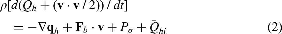
This article discusses a new approach for predicting and quantifying mechanically induced temperature oscillations in the coupled thermo-elasticity analysis of articulated mechanical systems (AMS). In this approach, the constrained equations of motion are solved simultaneously with discrete temperature equations obtained by converting heat partial-differential equation to a set of first-order ordinary differential equations. Dependence of the temperature gradients and their spatial derivatives on the position gradients, spinning motion, and curvatures is discussed. The approach captures dependence of the temperature-oscillation frequencies on the mechanical-displacement frequencies. The temperature field can be selected to ensure continuity of the temperature gradients at the nodal points. To generalize the AMS coupled thermo-elasticity formulation and capture the effect of the boundary and motion constraints (BMC) on the thermal expansion, the proposed method is based on integrating thermodynamics and Lagrange-D’Alembert principles. The absolute nodal coordinate formulation (ANCF) is used to describe continuum displacement and obtain accurate description of the reference-configuration geometry and change of this geometry due to deformations. A thermal-analysis large-displacement formulation is used to allow converting heat energy to kinetic energy, ensuring stress-free thermal expansion in case of unconstrained uniform thermal expansion. Cholesky heat coordinates are used to define an identity coefficient matrix for the efficient solution of the discretized heat equations. The approach presented is applicable to the two different forms of the heat equation used in the literature; one form is explicit function of the stresses while the other form does not depend explicitly on the stresses. Because of the need for using ANCF finite elements to achieve a higher degree of continuity in the coupled thermomechanical approach introduced in this article, the concept of the ANCF mesh topology is discussed.

Introduction

The thermodynamics energy balance is used in the literature to obtain a general form of the heat partial-differential equation.^1–5 This equation is function of the temperature gradients and their spatial derivatives defined in the current configuration. Capturing the effect of mechanically induced temperature oscillations due to the continuum spinning motion and large deformations requires accurate description of the geometry. Nonetheless, the literature lacks a Lagrangian approach for predicting and quantifying mechanically induced temperature oscillations in the coupled thermo-elasticity analysis of articulated mechanical systems (AMS). Consequently, there is no computational algorithm for solving constrained dynamic equations of motion simultaneously with the discrete temperature equations, which can be obtained by converting heat partial-differential equation to a set of first-order ordinary differential equations. If the rate of heat input to the continuum is not oscillatory, the only source of temperature oscillations is attributed to mechanical oscillations due to rotations and deformations. Because of the lack of AMS-coupled thermo-elasticity formulation, the dependence of the temperature gradients and their spatial derivatives on the continuum position gradients, spinning motion, and curvatures is not well understood and cannot be accurately quantified. Furthermore, dependence of temperature-oscillation frequencies on mechanical-displacement frequencies cannot be captured accurately without accurate geometry representation. To generalize AMS-coupled thermo-elasticity formulations and capture effect of boundary and motion constraints (BMC) on the thermal expansion, an approach based on integrating thermodynamics and Lagrange-D’Alembert principles is needed. Using Lagrange-D’Alembert principle is necessary for proper treatment of the BMC restrictions. Furthermore, because of the dependence of the temperature gradients on the curvatures, a finite element (FE) interpolation for accurate description of the reference-configuration geometry and change of this geometry due to deformations is required for correct prediction of the temperature oscillations.

To address these challenges, a Lagrangian approach approach for predicting and quantifying mechanically induced temperature oscillations in the AMS-coupled thermo-elasticity analysis is introduced. In this approach, the constrained equations of motion are solved simultaneously with the discrete temperature equations obtained by converting heat partial-differential equation to a set of first-order ordinary differential equations using FE interpolations. The dependence of the temperature gradients and their spatial derivatives on the position gradients, spinning motion, and curvatures is demonstrated. The approach captures dependence of temperature-oscillation frequencies on the mechanical-displacement frequencies. Furthermore, the FE temperature field can be selected to ensure continuity of the temperature gradients at the nodal points. The AMS coupled thermo-elasticity formulation is based on integrating thermodynamics and Lagrange-D’Alembert principles to capture the effect of BMC restrictions on the thermal expansion. The absolute nodal coordinate formulation (ANCF) is used to describe continuum displacement and obtain accurate description of the reference-configuration geometry and change of this geometry due to deformations. This can be conveniently achieved by using continuum-mechanics position gradients.^6–9 To allow converting heat energy to kinetic energy, a thermal-analysis large-displacement formulation is used to ensure stress-free thermal expansion in the absence of BMC restrictions and forces. This is achieved by using a sweeping-matrix technique to eliminate rigid-body translational modes from thermal-displacement field. Efficient solution of the coupled constrained motion and heat equations can be obtained using Cholesky heat coordinates, which lead to an identity coefficient matrix of the discretized heat equations. Using Cholesky heat coordinates in the numerical implementation is important in cases in which the rate of heat energy input depends on the motion accelerations. In the special cases that may arise in contact and friction problems, using Cholesky coordinates leads to an optimum sparse matrix structure for the augmented form of the motion-heat equations.

Because of the dependence of temperature gradients and their derivatives on the position gradients and curvatures, using ANCF finite elements is necessary. In the literature, different ANCF elements with different coordinate types are introduced. In some of these elements, curvature coordinates are used leading to different continuity conditions at the element interface. It is suggested in some studies that the choice of coordinates can offer solution to the locking problems without addressing the issues of compliance and articulation of the ANCF mesh. More research is needed to distinguish between locking and mobility of the ANCF mesh. This important and new area of ANCF mesh topology is also discussed in this article because of its relevance to the degree of continuity and displacement frequencies that influence mechanically induced temperature oscillations.

Thermodynamics and motion equations

The principle of thermodynamics and time-rate of energy flow can be used to derive the heat equation and demonstrate its coupling with the motion equation. Crucial in developing this principle is the definition of the power of the stress force $P_{\sigma }$ . There are two forms of the heat equation used in the solid-mechanics and FE literature. One form is not explicit function of the stresses, and the other form is explicit function of the stresses and rate of deformation tensor. The difference between the two forms can be attributed to two different definitions of the stress-force vector. Nonetheless, both forms of the heat equation exhibit clear geometric coupling with the equations of motion of the continuum. While this geometric coupling is the focus of this study, a discussion of the two different forms of the heat equation is presented in this section.

Motion and thermodynamics relationship

If $\mathbf{r}={\left[\begin{array}{ccc}{r}_1& r_2& r_3\end{array}\right]}^T$ is the position vector of a material point in the current configuration and $\mathbf{v}=\dot{\mathbf{r}}$ is its absolute velocity vector, one has $d({\mathbf{v}}^T\mathbf{v})/dt=2{\mathbf{v}}^T\dot{\mathbf{v}}=2{\mathbf{v}}^T\mathbf{a}$ , where $\mathbf{a}=\dot{\mathbf{v}}=\ddot{\mathbf{r}}$ is the absolute acceleration vector. That is, ${\mathbf{v}}^T\mathbf{a}=[d({\mathbf{v}}^T\mathbf{v})/dt]/2$ . The partial-differential equation of equilibrium can be written as $\rho \mathbf{a}={\mathbf{F}}_b+(\mathrm{\nabla }\sigma {)}^T$ ,^6–9 where $\rho$ is the mass density, ${\mathbf{F}}_b$ is the vector of body forces, $\mathrm{\nabla }$ is the row vector $\mathrm{\nabla }=\mathrm{\partial }/\mathrm{\partial }\mathbf{r}=\left[\begin{array}{ccc}\mathrm{\partial }/\mathrm{\partial }{r}_1& \mathrm{\partial }/\mathrm{\partial }{r}_2& \mathrm{\partial }/\mathrm{\partial }{r}_3\end{array}\right]$ , and $\sigma$ is the symmetric Cauchy-stress tensor. Important to the discussion presented in this section is the fact that the stress-force vector in the motion equation $\rho \mathbf{a}={\mathbf{F}}_b+(\mathrm{\nabla }\sigma {)}^T$ is defined as ${\mathbf{F}}_{\sigma }=(\mathrm{\nabla }\sigma {)}^T$ .

Multiplying the partial-differential equation of equilibrium $\rho \mathbf{a}={\mathbf{F}}_b+(\mathrm{\nabla }\sigma {)}^T$ by the absolute velocity vector $\mathbf{v}$ , one obtains $\rho \mathbf{a}\cdot \mathbf{v}={\mathbf{F}}_b\cdot \mathbf{v}+(\mathrm{\nabla }\sigma )\mathbf{v}$ . Substituting the identity ${\mathbf{v}}^T\mathbf{a}=[d({\mathbf{v}}^T\mathbf{v})/dt]/2$ into this equation leads to the force-power equation

$$\rho [d({\mathbf{v}}^T\mathbf{v})/dt]/2={\mathbf{F}}_b\cdot \mathbf{v}+(\mathrm{\nabla }\sigma )\mathbf{v}$$

(1)

In this equation, the power of the stress-force vector is defined as $P_{\sigma m}={\mathbf{F}}_{\sigma }\cdot \mathbf{v}=(\mathrm{\nabla }\sigma )\mathbf{v}$ . This definition is based on using the stress-force vector that contributes to the continuum motion. At this point, distinction is made between $P_{\sigma }$ and $P_{\sigma m}$ to allow explaining the difference between the two forms of the heat equation used in the literature.

The thermodynamics energy balance can be written as^1–5

$$\rho [d(Q_h+(\mathbf{v}\cdot \mathbf{v}/2))/dt]=-\mathrm{\nabla }{\mathbf{q}}_h+{\mathbf{F}}_b\cdot \mathbf{v}+P_{\sigma }+{\overline{Q}}_{hi}$$

(2)

where $Q_h$ is the thermodynamics energy at the microscopic level, ${\mathbf{q}}_h$ is the rate of heat energy flow, $P_{\sigma }$ is the power of the stress forces, and ${\overline{Q}}_{hi}$ is the rate of external heat input. Equations 1 and 2 lead to the heat equation

$$\rho (d{Q}_h/dt)=-\mathrm{\nabla }{\mathbf{q}}_h+(P_{\sigma }-(\mathrm{\nabla }\sigma )\mathbf{v})+{\overline{Q}}_{hi}$$

(3)

Therefore, the continuum motion and temperature distribution are governed by the following coupled motion and heat equations:

$$\begin{array}{c}\rho \mathbf{a}={\mathbf{F}}_b+(\mathrm{\nabla }\sigma {)}^T\\ \rho (d{Q}_h/dt)=-\mathrm{\nabla }{\mathbf{q}}_h+(P_{\sigma }-(\mathrm{\nabla }\sigma )\mathbf{v})+{\overline{Q}}_{hi}\end{array}\}$$

(4)

The discretized form of the first equation, which is the partial-differential equation of equilibrium,^6–9 can be obtained using approximation methods as described in the FE and multibody system (MBS) literatures.^10–18 The motion of the continuum can be subjected to BMC which can be nonlinear functions in the generalized coordinates selected for the motion description.

Power of the stress forces

The temperature and displacement are independent fields despite coupling that may exist between them. Furthermore, independent interpolations are used for the two fields to obtain the discretized equations. The fact that the two fields are independent despite their influence on each other implies that temperature environment and motion can be controlled independently. For example, heating or cooling sources can be used to maintain constant temperature while the continuum is expanding (isothermal expansion). Therefore, the equations that govern the coupled thermomechanical systems must ensure the independence of the two fields.

The definition of the stress-force power $P_{\sigma m}=(\mathrm{\nabla }\sigma )\mathbf{v}$ is resulting from the partial-differential equation of equilibrium (Eq. 1). If $P_{\sigma }$ is assumed equal to $P_{\sigma m}$ , the heat equation reduces to $\rho (d{Q}_h/dt)=-\mathrm{\nabla }{\mathbf{q}}_h+{\overline{Q}}_{hi}$ , which is not an explicit function of the stresses. This form of the heat equation is used in the literature to formulate the coupled thermomechanical problems. In some texts, however, the power of the stress forces is assumed $P_{\sigma }=\mathrm{\nabla }(\sigma \mathbf{v})$ . The relationship between the two expressions is $\mathrm{\nabla }(\sigma \mathbf{v})=(\mathrm{\nabla }\sigma )\mathbf{v}+\sigma :(\mathrm{\partial }\mathbf{v}/\mathrm{\partial }\mathbf{r})$ , where $\mathrm{\partial }\mathbf{v}/\mathrm{\partial }\mathbf{r}=\mathbf{L}$ is the velocity gradient tensor, which can be written as $\mathbf{L}=\mathbf{D}+\mathbf{W}$ , where $\mathbf{D}$ is the symmetric rate of deformation tensor and $\mathbf{W}$ is the skew-symmetric spin tensor. Because $\sigma$ is symmetric, one has $\sigma :(\mathrm{\partial }\mathbf{v}/\mathrm{\partial }\mathbf{r})=\sigma :\mathbf{L}=\sigma :(\mathbf{D}+\mathbf{W})=\sigma :\mathbf{D}$ . Therefore, $P_{\sigma }=P_{\sigma m}+\sigma :\mathbf{D}$ , which upon substituting into the energy-balance rate equation leads to another form of the heat equation $\rho (d{Q}_h/dt)=-\mathrm{\nabla }{\mathbf{q}}_h+\sigma :\mathbf{D}+{\overline{Q}}_{hi}$ . The concern regarding this form of the heat equation is that the rate of internal energy $\sigma :\mathbf{D}$ becomes equal to zero in the case of uniform constant temperature. Temperature and motion coordinates, which can be coupled, can be varied independently, and therefore, creating temperature conditions that lead to zero $\sigma :\mathbf{D}$ requires further investigation that is beyond the scope of this study. This problem is attributed to the definition of the stress force and to whether $\mathrm{\nabla }(\sigma \mathbf{v})$ should be interpreted as the rate of total deformation energy or the rate of surface-stress energy. It can be shown that the volume integral of $\mathrm{\nabla }(\sigma \mathbf{v})$ leads to the power of the stress forces on the boundary, which is distinguished from the power of the stresses inside the continuum. The appendix of the article provides an argument for using $P_{\sigma }=P_{\sigma m}$ to define the heat equation used in thermodynamics texts. Some references on thermo-elasticity, on the other hand, assume the other case in which $P_{\sigma }\ne P_{\sigma m}$ .

Boundary and internal stresses

The discretized form of the motion equation allows for including prescribed stresses on the continuum surface. Therefore, one may argue that ${\mathbf{F}}_{\sigma m}=(\mathrm{\nabla }\sigma )\mathbf{v}$ includes the effect of both internal and surface stresses. In this case, the heat equation $\rho (d{Q}_h/dt)=-\mathrm{\nabla }{\mathbf{q}}_h+{\overline{Q}}_{hi}$ is used, with the understanding that it is derived using the power of the stress forces $P_{\sigma }=P_{\sigma m}=(\mathrm{\nabla }\sigma )\mathbf{v}$ , which also includes the effect of the surface stresses since the effect of the boundary-surface stresses cannot be ignored in the formulation of the motion equation. ⁹ This can be demonstrated by multiplying the partial-differential equation of equilibrium by the virtual change $\delta \mathbf{r}$ , where $\mathbf{r}$ is the position vector of an arbitrary material point in the current configuration. This leads to $\rho \mathbf{a}\cdot \delta \mathbf{r}={\mathbf{F}}_b\cdot \delta \mathbf{r}+(\mathrm{\nabla }\sigma )\delta \mathbf{r}$ . One can write the last term in this equation as $(\mathrm{\nabla }\sigma )\delta \mathbf{r}=\mathrm{\nabla }(\sigma \delta \mathbf{r})-\sigma :\mathrm{\nabla }(\delta \mathbf{r})$ . Using this identity in $\rho \mathbf{a}\cdot \delta \mathbf{r}={\mathbf{F}}_b\cdot \delta \mathbf{r}+(\mathrm{\nabla }\sigma )\delta \mathbf{r}$ and following the derivation presented on Page 106 of Reference, ⁹ one obtains ${\int }_s{\mathbf{n}}^T\sigma \delta \mathbf{r}ds-{\int }_v\sigma :(\delta \mathbf{J}){\mathbf{J}}^{-1}dv+{\int }_v{({\mathbf{F}}_b-\rho \mathbf{a})}^T\delta \mathbf{r}dv=0$ , where $\mathbf{n}$ is the normal to the surface, s and v are, respectively, the area and volume in the current configuration, and $\mathbf{J}$ is the matrix of position-gradient vectors. The term ${\int }_v\sigma :(\delta \mathbf{J}){\mathbf{J}}^{-1}dv$ can be expressed in terms of the strains demonstrating that both internal and surface stress forces are accounted for. ⁹ This simple analysis demonstrates that using $(\mathrm{\nabla }\sigma {)}^T$ as the stress-force vector does not exclude the effect of the boundary-surface stresses, which need to be differentiated from the surface traction defined at the body interior and used to develop Cauchy-stress formula.

Temperature partial-differential equation

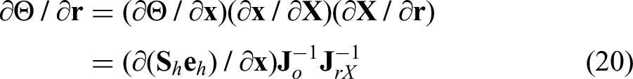
Because this study is mainly focused on the geometric thermomechanical coupling, both forms of the heat equations can be written as $\rho (d{Q}_h/dt)=-\mathrm{\nabla }{\mathbf{q}}_h+Q_{hi}$ , where $Q_{hi}={\overline{Q}}_{hi}+(P_{\sigma }-P_{\sigma m})$ . If $P_{\sigma }=P_{\sigma m}$ , one obtains the form of the heat equation which is not explicit function of the stresses; otherwise the second form of the heat equation which is explicit in the stresses is obtained. Therefore, the analysis presented in the remainder of this study is applicable to both forms.

The heat equation $\rho (d{Q}_h/dt)=-\mathrm{\nabla }{\mathbf{q}}_h+Q_{hi}$ can be written in terms of the temperatures $\mathrm{\Theta }$ by using Fourier's law of heat conduction ${\mathbf{q}}_h=-k_h\mathrm{\nabla }\mathrm{\Theta }=-k_h(\mathrm{\partial }\mathrm{\Theta }/\mathrm{\partial }\mathbf{r})$ , where $k_h$ is the coefficient of thermal conductivity which has units Watt/(m.K). Furthermore, the thermodynamics energy $Q_h$ can be written in terms of the change in the temperature using the relationship $\mathrm{\Delta }{Q}_h=\rho c_p\mathrm{\Delta }\mathrm{\Theta }$ , where $c_p$ is the specific heat. It follows that ${\dot{Q}}_h=d{Q}_h/dt=\rho c_p(d\mathrm{\Theta }/dt)$ , and the heat equation can be written as $\rho c_p(d\mathrm{\Theta }/dt)=\mathrm{\nabla }(k_h{\mathrm{\nabla }}_v\mathrm{\Theta })+Q_{hi}$ , where ${\mathrm{\nabla }}_v={\mathrm{\nabla }}^T$ . Therefore, the dynamics and temperature distribution of the continuum are governed by the two-coupled partial-differential equations:

$$\begin{array}{c}\rho \mathbf{a}={\mathbf{F}}_b+(\mathrm{\nabla }\sigma {)}^T\\ \rho c_p(d\mathrm{\Theta }/dt)=\mathrm{\nabla }(k_h{\mathrm{\nabla }}_v\mathrm{\Theta })+Q_{hi}\end{array}\}$$

(5)

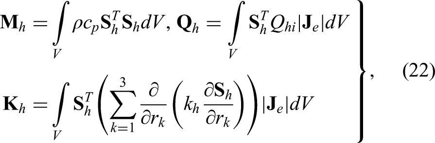
The discretized forms of these two-coupled equations and the numerical procedure for obtaining their solution will be discussed in later sections of this article.

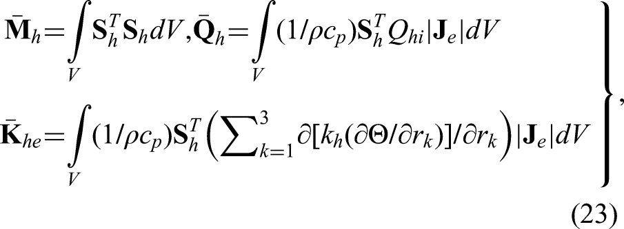
Mechanically induced thermal oscillations

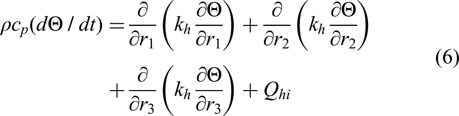
The heat equation can be written more explicitly in the following form:

$$\begin{array}{rl}\rho c_p(d\mathrm{\Theta }/dt)=& {\displaystyle \frac{\mathrm{\partial }}{\mathrm{\partial }{r}_1}\left(k_h{\displaystyle \frac{\mathrm{\partial }\mathrm{\Theta }}{\mathrm{\partial }{r}_1}}\right)+{\displaystyle \frac{\mathrm{\partial }}{\mathrm{\partial }{r}_2}\left(k_h{\displaystyle \frac{\mathrm{\partial }\mathrm{\Theta }}{\mathrm{\partial }{r}_2}}\right)}}\\ +& {\displaystyle \frac{\mathrm{\partial }}{\mathrm{\partial }{r}_3}\left(k_h{\displaystyle \frac{\mathrm{\partial }\mathrm{\Theta }}{\mathrm{\partial }{r}_3}}\right)+Q_{hi}}\end{array}$$

(6)

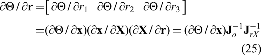
This explicit form of the heat equation demonstrates the dependence of the temperature on the reference-configuration geometry and mechanical displacement that can include rigid-body rotations. This dependence can be the result of the first three terms on the right-hand side of the preceding equation, and $Q_{hi}$ . Changes in position gradients due to rigid-body rotations and/or deformations contribute to changes in the first three terms. The term $Q_{hi}$ that includes prescribed rate of heat energy inputs can be function of the system dynamics as in case of contact and friction problems. Given rate of heat generated included in $Q_{hi}$ and vector of motion coordinate $\mathbf{q}$ at a specific time point t, the preceding equation can be solved using approximation methods to determine temperature $\mathrm{\Theta }$ as function of time at an arbitrary material point.

Position gradients and geometry

If the thermal conductivity coefficient within an element is assumed independent of the spatial coordinates, the spatial derivative on the right-hand side of the heat equation can be written as

$$\begin{array}{rl}& {\displaystyle \frac{\mathrm{\partial }}{\mathrm{\partial }{r}_1}\left({\displaystyle \frac{\mathrm{\partial }\mathrm{\Theta }}{\mathrm{\partial }{r}_1}}\right)+{\displaystyle \frac{\mathrm{\partial }}{\mathrm{\partial }{r}_2}\left({\displaystyle \frac{\mathrm{\partial }\mathrm{\Theta }}{\mathrm{\partial }{r}_2}}\right)+{\displaystyle \frac{\mathrm{\partial }}{\mathrm{\partial }{r}_3}\left({\displaystyle \frac{\mathrm{\partial }\mathrm{\Theta }}{\mathrm{\partial }{r}_3}}\right)={\sum }_{k=1}^3{\displaystyle \frac{\mathrm{\partial }}{\mathrm{\partial }{r}_k}\left({\displaystyle \frac{\mathrm{\partial }\mathrm{\Theta }}{\mathrm{\partial }{r}_k}}\right)}}}}\\ & ={\sum }_{k=1}^3{\sum }_{j=1}^3\left[{\displaystyle \frac{\mathrm{\partial }}{\mathrm{\partial }{x}_j}\left({\displaystyle \frac{\mathrm{\partial }\mathrm{\Theta }}{\mathrm{\partial }{r}_k}}\right)}\right]\left({\displaystyle \frac{\mathrm{\partial }{x}_j}{\mathrm{\partial }{r}_k}}\right)\end{array}$$

(7)

Let $\mathbf{x}={\left[\begin{array}{ccc}{x}_1& x_2& x_3\end{array}\right]}^T$ and $\mathbf{X}={\left[\begin{array}{ccc}{X}_1& X_2& X_3\end{array}\right]}^T$ be, respectively, the spatial coordinates in the straight and reference configurations before displacements. The reference configuration $\mathbf{X}$ defines the initial curved geometry, while the straight configuration $\mathbf{x}$ defines the straight un-curved geometry used to perform the integration in the FE analysis. The relationship between the two configurations is defined by the constant matrix ${\mathbf{J}}_o=\mathrm{\partial }\mathbf{X}/\mathrm{\partial }\mathbf{x}$ . It is clear that

$${\mathbf{J}}_e=\mathrm{\partial }\mathbf{r}/\mathrm{\partial }\mathbf{x}=(\mathrm{\partial }\mathbf{r}/\mathrm{\partial }\mathbf{X})(\mathrm{\partial }\mathbf{X}/\mathrm{\partial }\mathbf{x})={\mathbf{J}}_{rX}{\mathbf{J}}_o$$

(8)

where ${\mathbf{J}}_{rX}=\mathrm{\partial }\mathbf{r}/\mathrm{\partial }\mathbf{X}$ . That is, position-gradient matrix ${\mathbf{J}}_e$ accounts for the reference-configuration geometry that can be conveniently described using ANCF position gradients that allow for local shape manipulation. ¹⁹

Derivative evaluation

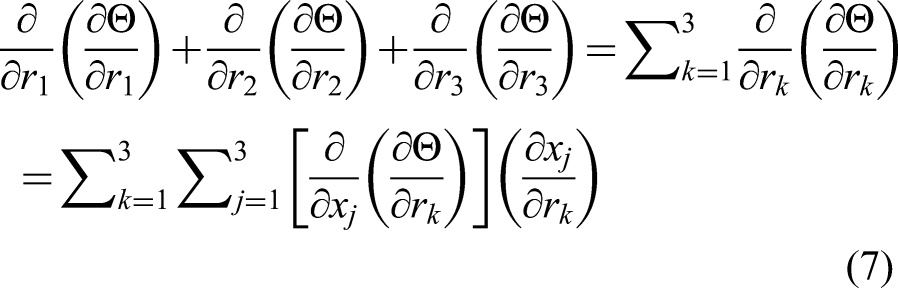
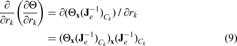
For efficient computer implementation, the spatial derivatives on the right-hand side of the heat equation need to be correctly evaluated to capture accurately effect of the reference-configuration geometry and deformation on the temperature oscillations. To this end, one can write $r_k=r_k(\mathbf{x}),k=1,2,3$ , $\mathrm{\partial }{r}_k/\mathrm{\partial }\mathbf{x}=\left[\begin{array}{cc}\mathrm{\partial }{r}_k/\mathrm{\partial }{x}_1& \mathrm{\partial }{r}_k/\mathrm{\partial }{x}_2\mathrm{\partial }{r}_k/\mathrm{\partial }{x}_3\end{array}\right]=({\mathbf{J}}_e{)}_{R_k}$ , where $({\mathbf{J}}_e{)}_{R_k}$ is the kth row of the position-gradient matrix ${\mathbf{J}}_e=\mathrm{\partial }\mathbf{r}/\mathrm{\partial }\mathbf{x}$ . It follows that ${\mathbf{J}}_e^{-1}=\mathrm{\partial }\mathbf{x}/\mathrm{\partial }\mathbf{r}$ and $\mathrm{\partial }\mathbf{x}/\mathrm{\partial }{r}_k=({\mathbf{J}}_e^{-1}{)}_{C_k}$ , where $({\mathbf{J}}_e^{-1}{)}_{C_k}$ is the kth column of ${\mathbf{J}}_e^{-1}$ . Because for an arbitrary scalar a, $\mathrm{\partial }a/\mathrm{\partial }{r}_x=(\mathrm{\partial }a/\mathrm{\partial }\mathbf{x})(\mathrm{\partial }\mathbf{x}/\mathrm{\partial }{r}_x)=a_{\mathbf{x}}({\mathbf{J}}_e^{-1}{)}_{C_k}$ , one can write

$${\displaystyle \frac{\mathrm{\partial }}{\mathrm{\partial }{r}_k}\left({\displaystyle \frac{\mathrm{\partial }\mathrm{\Theta }}{\mathrm{\partial }{r}_k}}\right)=\mathrm{\partial }({\mathrm{\Theta }}_{\mathbf{x}}{({\mathbf{J}}_e^{-1})}_{C_k})/\mathrm{\partial }{r}_k=({\mathrm{\Theta }}_{\mathbf{x}}{({\mathbf{J}}_e^{-1})}_{C_k}{)}_{\mathbf{x}}({\mathbf{J}}_e^{-1}{)}_{C_k}}$$

(9)

In this equation, ${\mathrm{\Theta }}_{\mathbf{x}}=\left[\begin{array}{ccc}{\mathrm{\Theta }}_{x_1}& {\mathrm{\Theta }}_{x_2}& {\mathrm{\Theta }}_{x_3}\end{array}\right],{\mathbf{J}}_e^{-1}=\left[\begin{array}{c}{({\mathbf{J}}_e^{-1})}_{C_1}{({\mathbf{J}}_e^{-1})}_{C_2}{({\mathbf{J}}_e^{-1})}_{C_3}\end{array}\right]$ , and $a_{x_k}=\mathrm{\partial }a/\mathrm{\partial }{x}_k,k=1,2,3$ , for any scalar or vector a. In a more explicit form, the preceding equation can be written as

$$\begin{array}{rl}{\displaystyle \frac{{\mathrm{\partial }}^2\mathrm{\Theta }}{\mathrm{\partial }{r}_k^2}=}& ({\mathrm{\Theta }}_{\mathbf{x}}{({\mathbf{J}}_e^{-1})}_{C_k}{)}_{\mathbf{x}}({\mathbf{J}}_e^{-1}{)}_{C_k}\\ =& [[\begin{array}{ccc}{\mathrm{\Theta }}_{\mathbf{x}{x}_1}{({\mathbf{J}}_e^{-1})}_{C_k}& {\mathrm{\Theta }}_{\mathbf{x}{x}_2}{({\mathbf{J}}_e^{-1})}_{C_k}& {\mathrm{\Theta }}_{\mathbf{x}{x}_3}{({\mathbf{J}}_e^{-1})}_{C_k}\end{array}]\\ & +[\begin{array}{ccc}{\mathrm{\Theta }}_{\mathbf{x}}{({({\mathbf{J}}_e^{-1})}_{C_k})}_{x_1}& {\mathrm{\Theta }}_{\mathbf{x}}{({({\mathbf{J}}_e^{-1})}_{C_k})}_{x_2}& {\mathrm{\Theta }}_{\mathbf{x}}{({({\mathbf{J}}_e^{-1})}_{C_k})}_{x_3}\end{array}]]({\mathbf{J}}_e^{-1}{)}_{C_k}\end{array}$$

(10)

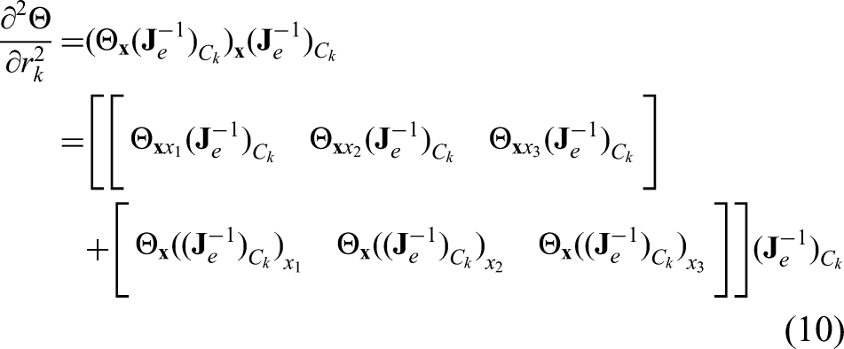
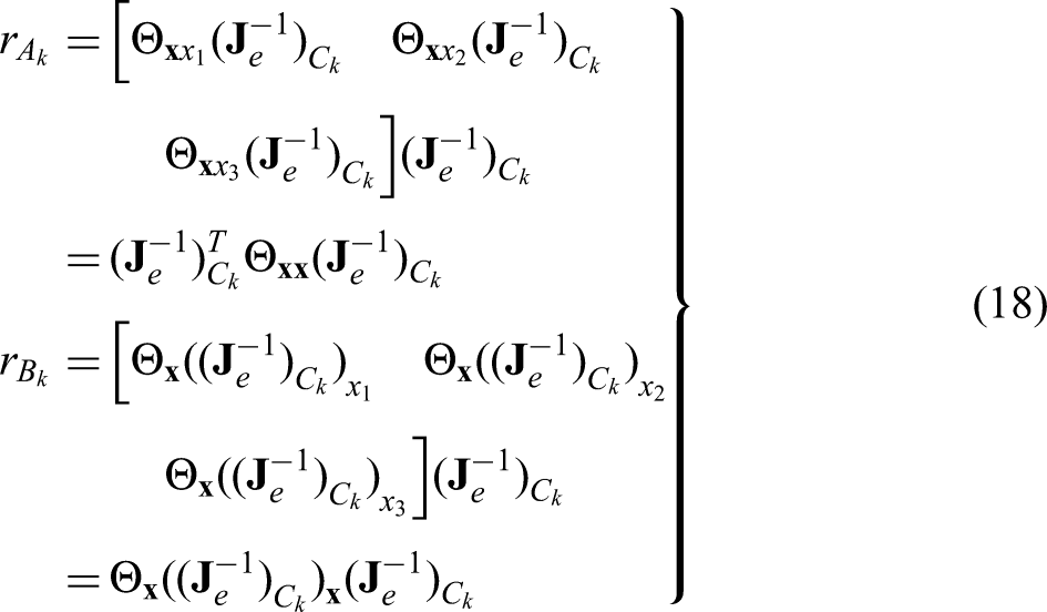
where ${\mathrm{\Theta }}_{\mathbf{x}{x}_k}=\left[\begin{array}{cc}({\mathrm{\partial }}^2\mathrm{\Theta }/\mathrm{\partial }{x}_1\mathrm{\partial }{x}_k)& ({\mathrm{\partial }}^2\mathrm{\Theta }/\mathrm{\partial }{x}_2\mathrm{\partial }{x}_k)({\mathrm{\partial }}^2\mathrm{\Theta }/\mathrm{\partial }{x}_3\mathrm{\partial }{x}_k)\end{array}\right]$ . Therefore, all the elements ${\mathrm{\Theta }}_{\mathbf{x}{x}_k}({\mathbf{J}}_e^{-1}{)}_{C_k},k=1,2,3$ on the right-hand side of the preceding equation can be found from the matrix multiplication ${\mathbf{\Theta }}_m{\mathbf{J}}_e^{-1}$ , where ${\mathbf{\Theta }}_m$ is the symmetric matrix

$$\begin{array}{rl}{\mathbf{\Theta }}_m& ={\mathrm{\Theta }}_{\mathbf{x}\mathbf{x}}=\left[\begin{array}{ccc}\left(\frac{{\mathrm{\partial }}^2\mathrm{\Theta }}{\mathrm{\partial }{x}_1^2}\right)& \left(\frac{{\mathrm{\partial }}^2\mathrm{\Theta }}{\mathrm{\partial }{x}_2\mathrm{\partial }{x}_1}\right)& \left(\frac{{\mathrm{\partial }}^2\mathrm{\Theta }}{\mathrm{\partial }{x}_3\mathrm{\partial }{x}_1}\right)\\ \left(\frac{{\mathrm{\partial }}^2\mathrm{\Theta }}{\mathrm{\partial }{x}_2\mathrm{\partial }{x}_1}\right)& \left(\frac{{\mathrm{\partial }}^2\mathrm{\Theta }}{\mathrm{\partial }{x}_2^2}\right)& \left(\frac{{\mathrm{\partial }}^2\mathrm{\Theta }}{\mathrm{\partial }{x}_3\mathrm{\partial }{x}_2}\right)\\ \left(\frac{{\mathrm{\partial }}^2\mathrm{\Theta }}{\mathrm{\partial }{x}_3\mathrm{\partial }{x}_1}\right)& \left(\frac{{\mathrm{\partial }}^2\mathrm{\Theta }}{\mathrm{\partial }{x}_3\mathrm{\partial }{x}_2}\right)& \left(\frac{{\mathrm{\partial }}^2\mathrm{\Theta }}{\mathrm{\partial }{x}_3^2}\right)\end{array}\right]\\ & =\left[\begin{array}{ccc}{\mathrm{\Theta }}_{x_1{x}_1}& & \\ {\mathrm{\Theta }}_{x_2{x}_1}& {\mathrm{\Theta }}_{x_2{x}_2}& \mathrm{symm}.\\ {\mathrm{\Theta }}_{x_3{x}_1}& {\mathrm{\Theta }}_{x_3{x}_2}& {\mathrm{\Theta }}_{x_3{x}_3}\end{array}\right]\end{array}$$

(11)

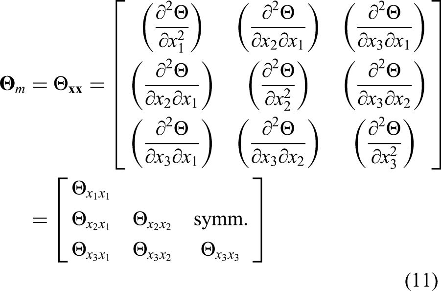
Similarly, all the elements ${\mathrm{\Theta }}_{\mathbf{x}}({({\mathbf{J}}_e^{-1})}_{C_k}{)}_{x_k},k=1,2,3$ , on the right-hand side of Eq. 10 can be found from the product ${\mathrm{\Theta }}_{\mathbf{x}}({\mathbf{J}}_e^{-1}{)}_{x_k},k=1,2,3$ , where $({\mathbf{J}}_e^{-1}{)}_{x_k}=\mathrm{\partial }{\mathbf{J}}_e^{-1}/\mathrm{\partial }{x}_k$ .

Inverse of position-gradient matrix

The method used to evaluate $({\mathbf{J}}_e^{-1}{)}_{x_k},k=1,2,3$ , is explained in this subsection. The differentiation of the inverse of the matrix of position-gradient vectors ${\mathbf{J}}_e$ can be avoided by using the identity ${\mathbf{J}}_e{\mathbf{J}}_e^{-1}=\mathbf{I}$ . Differentiating this equation with respect to $x_k$ and keeping in mind that ${\mathbf{J}}_e$ is always nonsingular matrix leads to $({\mathbf{J}}_e{)}_{x_k}{\mathbf{J}}_e^{-1}+{\mathbf{J}}_e({\mathbf{J}}_e^{-1}{)}_{x_k}=\mathbf{0}$ , which shows that

$$({\mathbf{J}}_e^{-1}{)}_{x_k}=-{\mathbf{J}}_e^{-1}({\mathbf{J}}_e{)}_{x_k}{\mathbf{J}}_e^{-1},k=1,2,3$$

(12)

That is, $({\mathbf{J}}_e^{-1}{)}_{x_k}$ can be evaluated from the curvature matrix

$$\begin{array}{rl}({\mathbf{J}}_e{)}_{x_k}=& \left[\begin{array}{ccc}({\mathrm{\partial }}^2\mathbf{r}/\mathrm{\partial }{x}_1\mathrm{\partial }{x}_k)& ({\mathrm{\partial }}^2\mathbf{r}/\mathrm{\partial }{x}_2\mathrm{\partial }{x}_k)& ({\mathrm{\partial }}^2\mathbf{r}/\mathrm{\partial }{x}_3\mathrm{\partial }{x}_k)\end{array}\right],\\ & k=1,2,3\end{array}$$

(13)

Therefore, the proposed coupled thermomechanical Lagrangian approach requires evaluation of second spatial derivatives of both temperature and the position coordinates. This is necessary to capture the effect of the geometry change on the heat equation. It is also clear that the resulting equations are nonlinear functions of the deformation coordinates that define the shape of the continuum.

Summary

The second derivatives on the right-hand side of the heat equation can be written as

$$({\mathrm{\partial }}^2\mathrm{\Theta }/\mathrm{\partial }{r}_k^2)=r_{A_k}+r_{B_k}$$

(14)

where

$$\begin{array}{rl}{r}_{A_k}=& \left[\begin{array}{ccc}{\mathrm{\Theta }}_{\mathbf{x}{x}_1}{({\mathbf{J}}_e^{-1})}_{C_k}& {\mathrm{\Theta }}_{\mathbf{x}{x}_2}{({\mathbf{J}}_e^{-1})}_{C_k}& {\mathrm{\Theta }}_{\mathbf{x}{x}_3}{({\mathbf{J}}_e^{-1})}_{C_k}\end{array}\right]({\mathbf{J}}_e^{-1}{)}_{C_k}\\ r_{B_k}=& \left[\begin{array}{ccc}{\mathrm{\Theta }}_{\mathbf{x}}{({({\mathbf{J}}_e^{-1})}_{C_k})}_{x_1}& {\mathrm{\Theta }}_{\mathbf{x}}{({({\mathbf{J}}_e^{-1})}_{C_k})}_{x_2}& {\mathrm{\Theta }}_{\mathbf{x}}{({({\mathbf{J}}_e^{-1})}_{C_k})}_{x_3}\end{array}\right]({\mathbf{J}}_e^{-1}{)}_{C_k}\end{array}\}$$

(15)

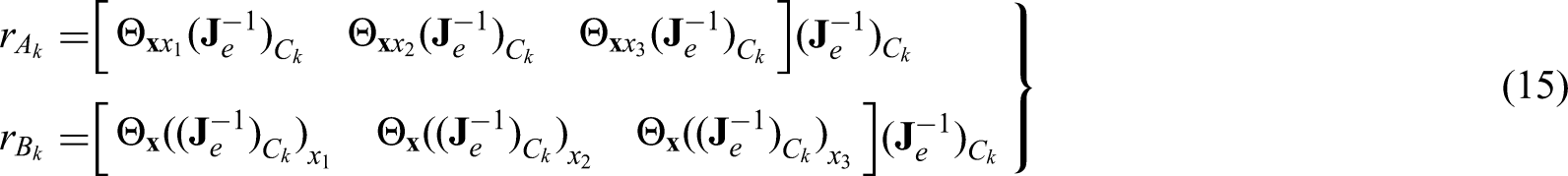
As previously mentioned, elements of the first equation in Eq. 15 be obtained by forming a matrix ${\mathbf{C}}_m=\left[\begin{array}{c}{\mathbf{C}}_1{\mathbf{C}}_2{\mathbf{C}}_3\end{array}\right]$ whose columns are defined by the vector

$${\mathbf{C}}_k^T=-{\mathrm{\Theta }}_{\mathbf{x}}({\mathbf{J}}_e^{-1}{({\mathbf{J}}_e^{-1})}_{x_k}{\mathbf{J}}_e^{-1}),k=1,2,3$$

(16)

Using these definitions, one can write

$$r_{B_k}=({\mathbf{C}}_m{)}_{R_k}({\mathbf{J}}_e^{-1}{)}_{C_k}$$

(17)

where $({\mathbf{C}}_m{)}_{R_k}$ is the kth row of the matrix ${\mathbf{C}}_m$ . Using the definition of ${\mathrm{\Theta }}_{\mathbf{x}}={\left[\begin{array}{ccc}{\mathrm{\Theta }}_{x_1}& {\mathrm{\Theta }}_{x_2}& {\mathrm{\Theta }}_{x_3}\end{array}\right]}^T$ and ${\mathbf{\Theta }}_m={\mathrm{\Theta }}_{\mathbf{x}\mathbf{x}}$ , one can write

$$\begin{array}{c}{r}_{A_k}=[{\mathrm{\Theta }}_{bfx{x}_1}{({bfJ}_e^{-1})}_{C_k}{\mathrm{\Theta }}_{bfx{x}_2}{({bfJ}_e^{-1})}_{C_k}\\ {\mathrm{\Theta }}_{bfx{x}_3}{({bfJ}_e^{-1})}_{C_k}]({bfJ}_e^{-1}{)}_{C_k}\\ =({bfJ}_e^{-1}{)}_{C_k}^T{\mathrm{\Theta }}_{bfxx}({bfJ}_e^{-1}{)}_{C_k}\\ r_{B_k}=[{\mathrm{\Theta }}_{bfx}{({({bfJ}_e^{-1})}_{C_k})}_{x_1}{\mathrm{\Theta }}_{bfx}{({({bfJ}_e^{-1})}_{C_k})}_{x_2}\\ {\mathrm{\Theta }}_{bfx}{({({bfJ}_e^{-1})}_{C_k})}_{x_3}]({bfJ}_e^{-1}{)}_{C_k}\\ ={\mathrm{\Theta }}_{bfx}(({bfJ}_e^{-1}{)}_{C_k}{)}_{bfx}({bfJ}_e^{-1}{)}_{C_k}\end{array}\}$$

(18)

Using these definitions for $r_{A_k}$ and $r_{B_k}$ allows efficient implementation of the heat equation in the coupled thermo-elasticity formulation introduced in this article. It is clear that motion frequencies influence the solution of the heat equation leading to mechanically induced temperature oscillations that contain frequencies defined by the mechanical oscillations.

Discretized heat equations

FE discretization methods can be applied to the heat partial-differential equation to obtain set of first-order-ordinary differential heat equations, which can be integrated with MBS algorithms to solve the coupled thermomechanical problem. Using an approach similar to the ANCF for the temperature interpolation, continuity of the temperature gradients and/or higher derivatives can be ensured. One can develop new ANCF temperature elements or use technique of separation of variables and write the temperature as

$$\mathrm{\Theta }(x_1,x_2,x_3,t)={\mathbf{S}}_h(x_1,x_2,x_3){\mathbf{e}}_h(t)$$

(19)

where ${\mathbf{S}}_h$ is space-dependent shape-function matrix, and ${\mathbf{e}}_h$ is time-dependent temperature-coordinate vector. The preceding equation and the ANCF displacement field $\mathbf{r}=\mathbf{S}(\mathbf{x})\mathbf{e}(t)$ lead to

$$\mathrm{\partial }\mathrm{\Theta }/\mathrm{\partial }\mathbf{r}=(\mathrm{\partial }\mathrm{\Theta }/\mathrm{\partial }\mathbf{x})(\mathrm{\partial }\mathbf{x}/\mathrm{\partial }\mathbf{X})(\mathrm{\partial }\mathbf{X}/\mathrm{\partial }\mathbf{r})=(\mathrm{\partial }({\mathbf{S}}_h{\mathbf{e}}_h)/\mathrm{\partial }\mathbf{x}){\mathbf{J}}_o^{-1}{\mathbf{J}}_{rX}^{-1}$$

(20)

While ${\mathbf{J}}_o=\mathrm{\partial }\mathbf{X}/\mathrm{\partial }\mathbf{x}$ is a constant matrix, ${\mathbf{J}}_{rX}$ depends on the ANCF displacement coordinates. The interpolation of $\mathrm{\Theta }$ can be selected to ensure continuity of $\mathrm{\Theta }$ , $\mathrm{\partial }\mathrm{\Theta }/\mathrm{\partial }{x}_k,k=1,2,3$ , and/or higher derivatives. The temperature and ANCF-element displacement meshes can be designed to have the same number of nodes and element sizes to simplify the computer implementation.

First-order ordinary heat equations

Using the interpolation $\mathrm{\Theta }={\mathbf{S}}_h{\mathbf{e}}_h$ , one can write $\delta \mathrm{\Theta }={\mathbf{S}}_h\delta {\mathbf{e}}_h$ and $\dot{\mathrm{\Theta }}={\mathbf{S}}_h{\dot{\mathbf{e}}}_h$ . Multiplying the heat equation by $\delta \mathrm{\Theta }$ , using $\mathrm{\Theta }={\mathbf{S}}_h{\mathbf{e}}_h$ and its time and spatial derivatives, pre-multiplying by ${\mathbf{S}}_h^T$ , and integrating over the volume, one can convert the partial-differential heat equation to the following set of first-order ordinary differential equations:

$${\mathbf{M}}_h{\dot{\mathbf{e}}}_h={\mathbf{K}}_h{\mathbf{e}}_h+{\mathbf{Q}}_h$$

(21)

where

$$\begin{array}{rl}{\mathbf{M}}_h=& \underset{V}{\int }\rho c_p{\mathbf{S}}_h^T{\mathbf{S}}_{h}dV,{\mathbf{Q}}_h=\underset{V}{\int }{\mathbf{S}}_h^T{Q}_{hi}|{\mathbf{J}}_e|dV\\ {\mathbf{K}}_h=& \underset{V}{\int }{\mathbf{S}}_h^T\left(\sum _{k=1}^3{\displaystyle \frac{\mathrm{\partial }}{\mathrm{\partial }{r}_k}\left(k_h{\displaystyle \frac{\mathrm{\partial }{\mathbf{S}}_h}{\mathrm{\partial }{r}_k}}\right)}\right)|{\mathbf{J}}_e|dV\end{array}\},$$

(22)

In this equation, $\rho$ and V are, respectively, mass density and volume in the straight configuration. While the matrix ${\mathbf{K}}_h$ is nonlinear function of the motion coordinates, the coefficient matrix ${\mathbf{M}}_h$ is constant. The matrix of position-gradient vectors ${\mathbf{J}}_e=\mathrm{\partial }\mathbf{r}/\mathrm{\partial }\mathbf{x}=(\mathrm{\partial }\mathbf{r}/\mathrm{\partial }\mathbf{X})(\mathrm{\partial }\mathbf{X}/\mathrm{\partial }\mathbf{x})={\mathbf{J}}_{rX}{\mathbf{J}}_o$ accounts for both deformations and reference-configuration geometry, demonstrating dependence of the integrals in the preceding equation on the initial geometry, deformations, and finite rotations.

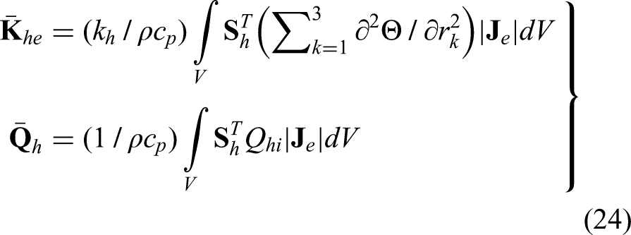
Numerical evaluation of the integrals

While vectors ${\mathbf{K}}_h{\mathbf{e}}_h$ and ${\mathbf{Q}}_h$ are nonlinear functions of the deformation coordinates, constant vectors and matrices can be identified and evaluated at a preprocessing stage. Such integrals can be efficiently evaluated using quadrature integration methods to ensure generality of the algorithm. To this end, the heat equations are written as ${\overline{\mathbf{M}}}_h{\dot{\mathbf{e}}}_h={\overline{\mathbf{K}}}_{he}+{\overline{\mathbf{Q}}}_h$ , where

$$\begin{array}{rl}{\overline{\mathbf{M}}}_h=& \underset{V}{\int }{\mathbf{S}}_h^T{\mathbf{S}}_{h}dV,{\overline{\mathbf{Q}}}_h=\underset{V}{\int }(1/\rho c_p){\mathbf{S}}_h^T{Q}_{hi}|{\mathbf{J}}_e|dV\\ {\overline{\mathbf{K}}}_{he}=& \underset{V}{\int }(1/\rho c_p){\mathbf{S}}_h^T\left({\sum }_{k=1}^3\mathrm{\partial }[k_h(\mathrm{\partial }\mathrm{\Theta }/\mathrm{\partial }{r}_k)]/\mathrm{\partial }{r}_k\right)|{\mathbf{J}}_e|dV\end{array}\},$$

(23)

Numerical integration methods allow using heat coefficients defined by empirical formulas or in a tabulated form. If the coefficient of thermal conductivity $k_h$ , mass density $\rho$ , and specific heat capacity $c_p$ are assumed constant within the element, the second and third integrals in the preceding equation can be written as

$$\begin{array}{rl}{\overline{\mathbf{K}}}_{he}& =(k_h/\rho c_p)\underset{V}{\int }{\mathbf{S}}_h^T\left({\sum }_{k=1}^3{\mathrm{\partial }}^2\mathrm{\Theta }/\mathrm{\partial }{r}_k^2\right)|{\mathbf{J}}_e|dV\\ {\overline{\mathbf{Q}}}_h& =(1/\rho c_p)\underset{V}{\int }{\mathbf{S}}_h^T{Q}_{hi}|{\mathbf{J}}_e|dV\end{array}\}$$

(24)

Evaluating ${\overline{\mathbf{K}}}_{he}$ integral requires having the inverse of ${\mathbf{J}}_e$ , as previously discussed. The resulting integral accounts for both initial geometry and change of the geometry due to deformation since

$$\begin{array}{rl}\mathrm{\partial }\mathrm{\Theta }/\mathrm{\partial }\mathbf{r}=& \left[\begin{array}{ccc}\mathrm{\partial }\mathrm{\Theta }/\mathrm{\partial }{r}_1& \mathrm{\partial }\mathrm{\Theta }/\mathrm{\partial }{r}_2& \mathrm{\partial }\mathrm{\Theta }/\mathrm{\partial }{r}_3\end{array}\right]\\ =& (\mathrm{\partial }\mathrm{\Theta }/\mathrm{\partial }\mathbf{x})(\mathrm{\partial }\mathbf{x}/\mathrm{\partial }\mathbf{X})(\mathrm{\partial }\mathbf{X}/\mathrm{\partial }\mathbf{r})=(\mathrm{\partial }\mathrm{\Theta }/\mathrm{\partial }\mathbf{x}){\mathbf{J}}_o^{-1}{\mathbf{J}}_{rX}^{-1}\end{array}$$

(25)

as discussed previously.

Cholesky heat coordinates

In some applications, mechanical energy dissipations due to contact and friction can lead to the dependence of the heat equation on the motion accelerations. If the rate of heat energy input $Q_{hi}$ becomes function of the motion accelerations, having sparse matrix structure can contribute significantly to the efficient solution of the coupled thermo-elasticity problem. An efficient general implementation can be achieved by applying Cholesky transformation to solve the first-order ordinary differential heat equations ${\overline{\mathbf{M}}}_h{\dot{\mathbf{e}}}_h={\overline{\mathbf{K}}}_{he}+{\overline{\mathbf{Q}}}_h$ for a given set of initial coordinates ${\mathbf{e}}_h$ . Using Cholesky heat coordinates ${\mathbf{e}}_{hC}$ leads to an identity coefficient matrix associated with these coordinates. The Cholesky coordinate transformation can be made because the matrix ${\overline{\mathbf{M}}}_h$ is symmetric and positive definite. Cholesky decomposition of this matrix ${\overline{\mathbf{M}}}_h={\mathbf{L}}_h{\mathbf{L}}_h^T$ can be used to define the Cholesky heat coordinate transformation ${\mathbf{e}}_h={\mathbf{L}}_h^{-T}{\mathbf{e}}_{hC}$ , which upon substituting into ${\overline{\mathbf{M}}}_h{\dot{\mathbf{e}}}_h={\overline{\mathbf{K}}}_{he}+{\overline{\mathbf{Q}}}_h$ and pre-multiplying by ${\mathbf{L}}_h^{-1}$ leads to ${\dot{\mathbf{e}}}_{hC}={\mathbf{L}}_h^{-1}({\overline{\mathbf{K}}}_{he}+{\overline{\mathbf{Q}}}_h)$ . Since ${\overline{\mathbf{M}}}_h$ is constant, the transformation ${\mathbf{L}}_h^{-T}$ is evaluated only once in advance of the dynamic simulations.

Effect of boundary and motion constraints

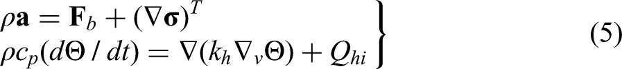
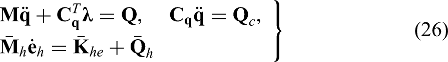
In case of stress-free thermal expansion, there is no oscillations in the position gradients. Consequently, there are no mechanically induced temperature oscillations. This is not the case if there is variation in the temperature gradients or if the continuum is subjected to BMC restrictions. The resulting stress oscillations lead to mechanically induced temperature oscillations that have the same frequency contents that characterize the elastic displacements and/or rigid-body spinning motion. The heat equation formulated in the current configuration demonstrates clearly the dependence of temperature on these two types of mechanical displacements; deformation and rotation. Using ANCF finite elements, the formulation of the heat equation can capture accurately arbitrary reference-configuration curved geometry. The vector $\mathbf{r}$ is written using ANCF approach as $\mathbf{r}=\mathbf{S}(\mathbf{x})\mathbf{e}(t)$ , where $\mathbf{S}$ and $\mathbf{e}$ are, respectively, ANCF-element shape-function matrix and nodal coordinate vector. ¹⁹ Therefore, in the coupled thermomechanical formulation proposed in this investigation, the partial-differential heat equation is solved simultaneously with the constrained MBS equations of motion, which are formulated using Lagrange-D’Alembert principle and can be written as $\mathbf{M}\ddot{\mathbf{q}}+{\mathbf{C}}_{\mathbf{q}}^T\lambda =\mathbf{Q}$ and ${\mathbf{C}}_{\mathbf{q}}\ddot{\mathbf{q}}={\mathbf{Q}}_c$ , where $\mathbf{M}$ is the system mass matrix, $\mathbf{q}$ is the MBS coordinate vector that includes the coordinate vector $\mathbf{e}$ used to describe the displacement of ANCF bodies and other coordinates used to describe the displacements of rigid bodies and bodies modeled using the floating frame of reference (FFR) formulation, $\mathbf{C}$ is the vector of constraint functions, ${\mathbf{C}}_{\mathbf{q}}=\mathrm{\partial }\mathbf{C}/\mathrm{\partial }\mathbf{q}$ is the constraint Jacobian matrix, $\lambda$ is the vector of Lagrange multipliers, $\mathbf{Q}$ is the applied-force vector that includes external, elastic, and quadratic-velocity inertia forces, and ${\mathbf{Q}}_c$ is the vector resulting from differentiation of the constraint equations twice with respect to time excluding terms which are linear in the accelerations.^16,20,21 Therefore, in this investigation, the following three matrix equations are solved simultaneously:

$$\begin{array}{c}\mathbf{M}\ddot{\mathbf{q}}+{\mathbf{C}}_{\mathbf{q}}^T\lambda =\mathbf{Q},{\mathbf{C}}_{\mathbf{q}}\ddot{\mathbf{q}}={\mathbf{Q}}_c,\\ {\overline{\mathbf{M}}}_h{\dot{\mathbf{e}}}_h={\overline{\mathbf{K}}}_{he}+{\overline{\mathbf{Q}}}_h\end{array}\}$$

(26)

This mathematical model is based on integrating Lagrange-D’Alembert principle for the treatment of the constraint equations and the principle of thermal analysis with the goal of capturing the effect of the geometric and kinematic changes on the temperature gradients. The effect of the heat energy on the constrained system dynamics is considered by using the thermo-elasticity displacement formulation, which is based on converting the heat energy to macroscopic kinetic energy. ²² By using a sweeping-matrix technique to eliminate rigid-body translations from thermal expansion modes of displacements, the thermal-analysis displacement approach ensures stress-free thermal expansion in case of uniform temperature and in the absence of BMC restrictions. Four configurations are used in the thermo-elasticity displacement formulation: straight, reference, thermal expansion, and current configurations.^21–23 Using these four configurations, the thermal-analysis large-displacement formulation is based on the multiplicative decomposition of the matrix of position gradients.^24–33 Furthermore, the formulation presented in this study can be used for the analysis of bodies modeled using the FFR formulation, using FFR/ANCF elements, ³⁴ and bodies with complex geometries and joints using the concept of the ANCF reference node.^17,35,36 Matrix sparsity ensures efficient numerical solution of the resulting coupled thermo-elasticity equations. ³⁷

As explained in, ²² the increase in temperature of the flexible bodies due to heat energy defines thermal displacement, which is used to formulate a kinetic energy function. The part of the heat energy dissipated to the environment does not contribute to increasing the flexible-body temperature, and this part of heat energy is not considered in this study. Furthermore, there is no thermal expansion of rigid bodies, which do not deform; therefore, the focus in this study is on ANCF bodies and on heat conduction. Heat convection and radiation are not considered in this study. Because the thermal expansion is described using the deformation coordinates and the MBS joint constraints are formulated in terms of the deformation coordinates, the heat energy has direct influence on the joint constraint equations.

ANCF mesh topology

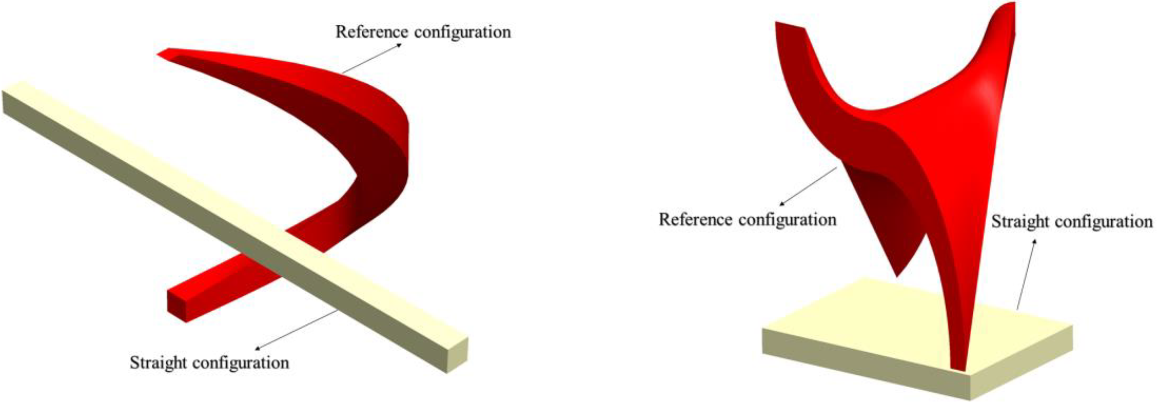
The analysis presented in the preceding sections demonstrates the need for using geometrically accurate analysis approach to predict correctly the influence of the mechanical oscillations on the temperature and its gradients. It is shown that the temperature gradients and their derivatives depend on the position gradients and curvature vectors. For this reason, the approach used in the deformation analysis can have significant effect on the accuracy of the solution of the coupled thermomechanical problem. ANCF finite elements can describe accurately reference-configuration geometry and change of this geometry due to deformations. These elements have been widely used in the nonlinear analysis of a wide range of challenging applications, some of which have complex geometry.^38–158 Figure 1 shows examples of geometries that can be obtained with two planar-beam and two spatial-plate elements. ¹⁹ The complex shapes, shown in the figure and obtained using ANCF elements, demonstrate the potential of using this approach in numerous applications including morphing applications.

Figure 1.

ANCF geometry. ¹⁹

In the literature, different ANCF elements with different coordinate types are introduced. In some of these elements, curvature coordinates are used leading to different levels of continuity conditions associated with different coordinates at the element interface. It was suggested in some studies that the choice of coordinates can offer solution to the locking problems without addressing the issues of compliance and articulation of the ANCF mesh. Locking is an issue that cannot be ignored in all FE formulations, including the conventional formulations. Nonetheless, interpretations of locking and their relationship to the choice of the ANCF coordinates are important issues that will require thorough future investigations. This is mainly because in case of ANCF elements, different choices of coordinates lead to different compliances and articulation freedom. For example, given an interpolating polynomial for the position vector $\mathbf{r}$ of an arbitrary point on the element, one can select different gradient and/or curvature coordinates as nodal coordinates to replace the polynomial coefficients. For one element, different choices of coordinate sets are related by a linear map, and therefore, regardless of the coordinates selected, a one-element mesh has the same response and the solution contains the same frequencies. However, when elements are connected to form multi-element mesh, the joints between elements are different, and different meshes that use different types of coordinates do not have the same response because of the type of joints used to connect the elements. That is, while one-element meshes based on different coordinate types lead to the same solution for any loading due to using the same interpolating polynomials, multi-element meshes can have different responses and can have different levels of stiffness in response to different loadings.

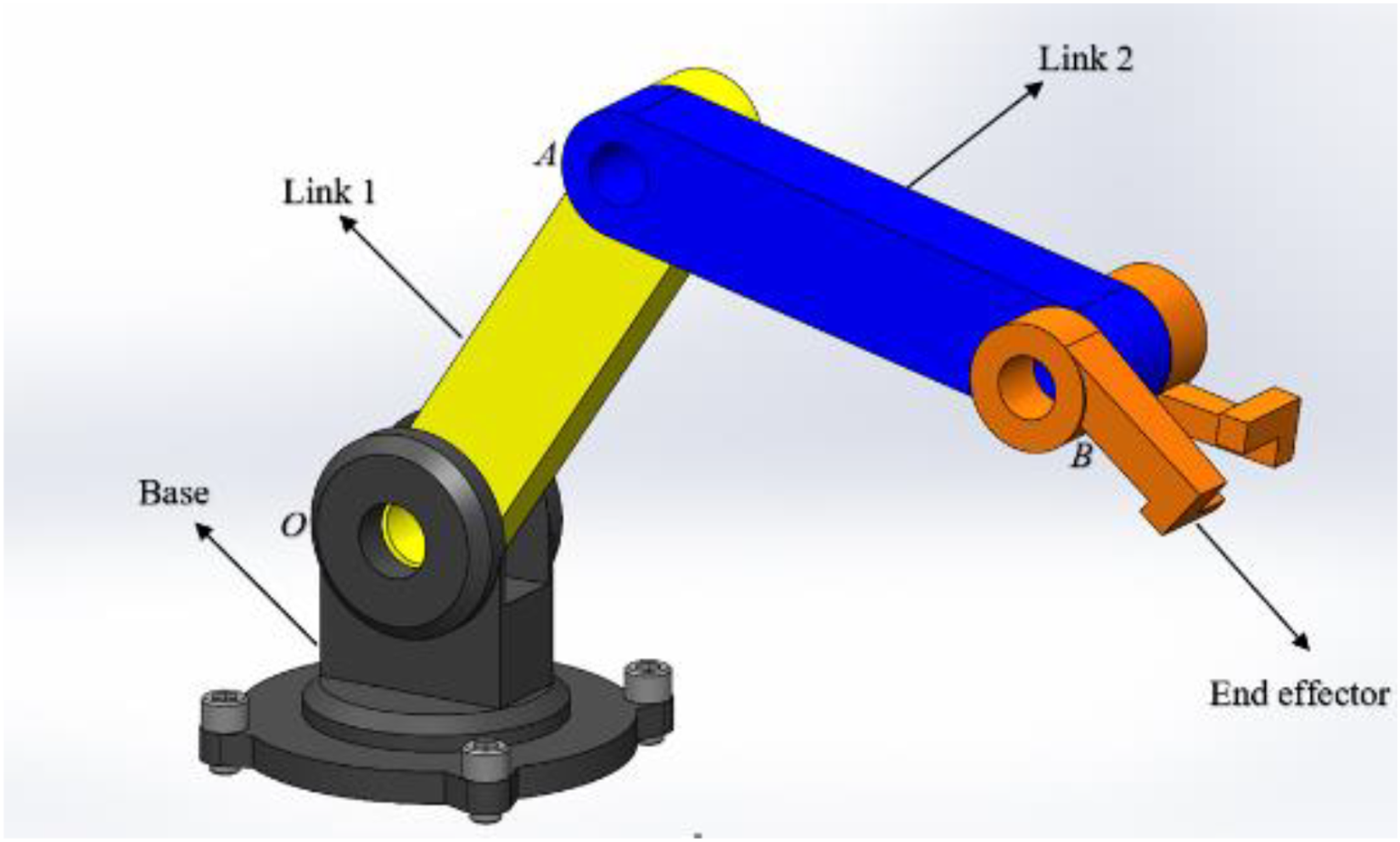
This important concept of the ANCF mesh topology can be better explained using the articulated-robot system shown in Figure 2. ¹⁵⁹ The links, which are connected by pin joints cannot be translated relative to each other and cannot have relative rotations about axes perpendicular to the joint axes regardless of the load applied. The pin joint does not transmit moment, and one link is free to rotate with respect to the other without resistance if the joint does not have compliance or friction. The same concept can be applied to ANCF elements to have proper interpretations of locking. Imposing higher degree of continuity increases the stiffness in certain directions, while excluding some gradients as nodal coordinates reduces stiffness in other direction. Therefore, choice of the type of the ANCF coordinates can be viewed as mesh-topology design that can be appropriate for some loading conditions and can lead to stiffness problems in other loading scenarios. However, not using all the gradients as nodal coordinates leads to rotation, strain, and stress discontinuities. More research is needed to distinguish between locking and mobility of the ANCF mesh. This important and new area of ANCF mesh topology is relevant to the coupled thermomechanical approach in which temperature and its spatial derivatives depend on the position gradients and their spatial derivatives including curvature vectors. ¹⁶⁰

Figure 2.

Mechanical system articulation. ¹⁵⁹

Summary

This article presents a Lagrangian approach for predicting and quantifying mechanically induced temperature oscillations in the AMS coupled thermo-elasticity problem. Constrained motion equations and discrete temperature equations obtained from heat partial-differential equation are solved simultaneously to capture the coupling between temperature and mechanical displacements. The discretized temperature first-order ordinary differential equations are obtained from the heat partial-differential equations using FE interpolations that can be selected to ensure continuity of temperature gradients. Dependence of temperature gradients and their spatial derivatives on position gradients, spinning motion, and curvatures and dependence of temperature-oscillation frequencies on mechanical-displacement frequencies are captured. The AMS coupled thermo-elasticity formulation, based on integrating thermodynamics and Lagrange-D’Alembert principles, captures BMC effect on the thermal expansion. ANCF finite elements are used to describe accurately large displacement, reference-configuration geometry, and geometry change due to deformations. Conversion of the heat energy to kinetic energy can be achieved by using a thermal-analysis large-displacement formulation to ensure stress-free thermal expansion in case of unconstrained uniform thermal expansion. ²² This thermal-analysis large-displacement formulation is based on the multiplicative decomposition of the matrix of position gradients.^24–33 Cholesky heat coordinates are used to define an identity coefficient matrix when solving discretized heat equations. ¹⁶¹ The formulation presented in this study can be used for the analysis of bodies modeled using the FFR formulation, using FFR/ANCF elements, ³⁴ and bodies with complex geometries and joints using the concept of the ANCF reference node.^17,35,36 Furthermore, the matrix sparsity achieved allows for efficient numerical solution of the resulting coupled thermo-elasticity equations. ³⁷ Because of the dependence of the heat equation on the continuum geometry, the ANCF mesh topology is expected to be an issue in future investigations. Enhancing the efficiency of the FE implementation is an important issue given recent research activities focused on developing new nonlinear formulations to address a wide range of challenging applications. While some of these investigations consider coupled ANCF thermomechanical analysis, the problem of large-displacement geometrically coupled analysis using ANCF finite elements as presented in this study has not been previously addressed.