
Abstract
This work presents a novel continuously differentiable, dynamic dry friction model, with dependence on normal contact force, slip velocity, and static and dynamic coefficients of friction. The state-of-the-art, Brown and McPhee friction model depends on transitional velocity, which is an empirical parameter. A limitation with this model is that there is no generic approach to select the optimal value for the transitional velocity for a certain application. The simulation results presented in this work highlight the sensitivity of friction force with transitional velocity in Brown and McPhee’s model to obtain smooth solutions, which are supportive in control system applications. It is because control systems require jitter-free signals in order to save costs on low-pass filters. The proposed model overcomes such empirical dependence on transition velocity through a combination of an iterative methodology and an empirical parameterization. In this article, a comprehensive analysis of the proposed friction model and the contributing parameters is carried out. The algorithm to implement the proposed friction model is elaborated. The proposed friction model is then simulated and compared against Brown and McPhee’s model. using a stick-slip benchmark problem. Furthermore, the proposed force model is applied to two spatial multibody systems formulated using index 0 tangent space differential-algebraic equations. The results demonstrate how the proposed friction model can be employed in dynamical mechanical systems. The independence on transitional velocity in the proposed friction model is observed to be effective for obtaining smooth solutions that make it suitable for control system applications.
Introduction
Friction is a highly nonlinear and complex phenomenon related to the resistance to the relative motion of bodies in contact. The very first attempts to model friction phenomena include,1,2 and since then, friction’s properties have been intensively studied, modeled, and used to predict frictional behavior in mechanical systems. The earliest friction force model dates to Coulomb’s friction force model. 3 According to this model, the friction force always opposed the relative motion between two surfaces and it is proportional to the normal force. While it was established that the friction force opposes relative motion, the Stribeck effect laid out that static friction was always higher than kinetic friction4,5 and showed experimentally that the transition from static to kinetic friction is a continuous process. This means that for low velocities, the friction force decreases with the increase in the relative velocity. This rise of friction force combined with a drop in the relative velocity leads to a phenomenon called “stick-slip” where the contact surfaces stick until the static friction is overcome.
Coulomb friction
Though Coulomb’s model is fundamental, it is quite basic when it comes to differentiating between static and dynamic regions of friction and hence Coulomb’s model is a static model since it disregards the existence of the two distinct types of friction regimes. The Stribeck model, although it considers the transition from static to dynamic friction, it does not do so in a continuous manner. Both, Coulomb’s model and Stribeck model are discontinuous and not continuously differentiable. This makes them further difficult to implement in the case studies where continuous derivatives of friction forces are required, 6 for example, in applications related to sensitivity analysis, optimal control, and multibody systems simulations with friction. Furthermore, Haug suggests that introducing friction prevents the formulation of an ordinary differential equation from accurately describing the dynamic characteristics of a system.7–10 Hence, a problem where friction must be considered needs to be formulated as a system of differential-algebraic equations (DAEs) with Lagrangian multipliers. Since the friction force depends on the normal contact force, the formulation with friction required derivatives of the external forces to satisfy the DAEs. This has been discussed in detail in subsequent sections.
Brown and McPhee’s friction model
As discussed, there is a need for a continuously differentiable friction force model that could also capture the transition of friction forces from a static to a dynamic state. Several continuous models of friction already exist. However, they neglect some of the crucial phenomena associated with friction. Berger’s model
11
neglects time lag in friction. Another important contribution by Armstrong-He’louvry et al.
12
proposes a continuous velocity-based model which captures the time-lag. However, it takes the absolute magnitudes of static and dynamic friction forces as inputs, instead of evaluating them through the magnitude of normal reaction. Certain models, based on the concept of bristle deflection, propose the usage of a state-variable to capture the micro-slip phenomena.13,14 However, these models are more complex and often discontinuous because of addition of state variables, which in turn makes them computationally inefficient. Bristle deflection models
13
also do not consider the velocity dependence of friction but only displacement dependence. Due to their more complex and less efficient nature, models that include such effects are not considered for this study. Readers are advised to refer to Marques et al.15,16 for more insight into the comparison of these friction models. Brown and McPhee
17
proposed a simple velocity-based model where friction has been considered as a continuous function of relative sliding velocity. They also compare their model with certain other contemporary continuous friction models, such as Andersson et al.’s,
14
Hollars,
18
and Specker’s model.
19
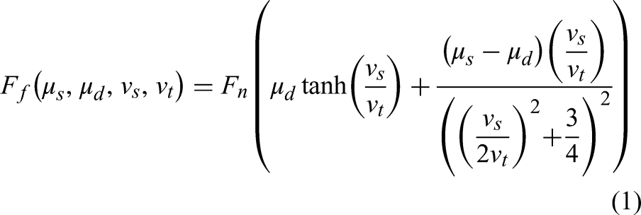
To reduce model complexity, only the main velocity-dependent characteristics of friction, that is, the Stribeck effect and viscous friction were included. What makes this friction model especially promising for dynamic systems is its ability to simulate stiction without any discontinuities in the stick-slip transition regime. This model, neglecting the viscous friction, is represented in equation (1)
Static friction model
Another friction model has been studied and proposed by Wang and Rui,
20
as provided in equation (2)

Limitations of friction models in dynamical systems
Acknowledging the impact of Brown and McPhee’s model and yet considering the drawbacks associated with it, this study focuses on an alternative model which does not include the selection of optimal
Proposed friction model
Model description
In the previous section, it was outlined why the Brown and McPhee friction model outperforms other dynamic friction models. Also, a static friction model by Wang and Rui
20
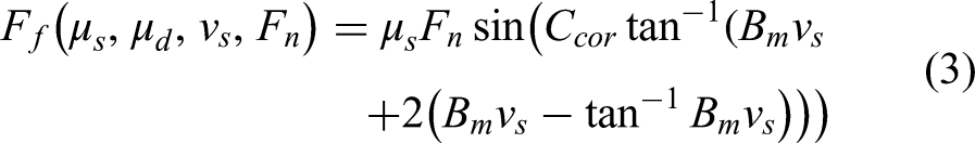
was revisited, as per equation (2). It is seen from the Rui and Wang’s model that the friction force is continuously differentiable; however, it is independent of the dynamic terms namely the dynamic coefficient of friction, the normal force, and the transitional velocity, thus rendering the model useful only in static applications. The proposed friction model is motivated by the limitations of these models, and it proposes modifying the Rui and Wang’s model to leverage its benefits in terms of continuous differentiability as well as independence on transitional velocity. The proposed friction model is as follows

Algorithm to obtain corrected model parameters
The value of
The function receives the values of coefficients of friction The factor The initial value of friction force Depending on the difference between The corrected parameter
Comparison of friction force models
From equations (2) and (3), it is seen that the friction force is a function of the slip velocity. The Brown and McPhee model, on the other hand, also depends on the transitional velocity, as mentioned earlier. The force profiles are plotted in Figure 1. The friction force profile is obtained for a given range of the slip velocity while keeping the normal force constant at
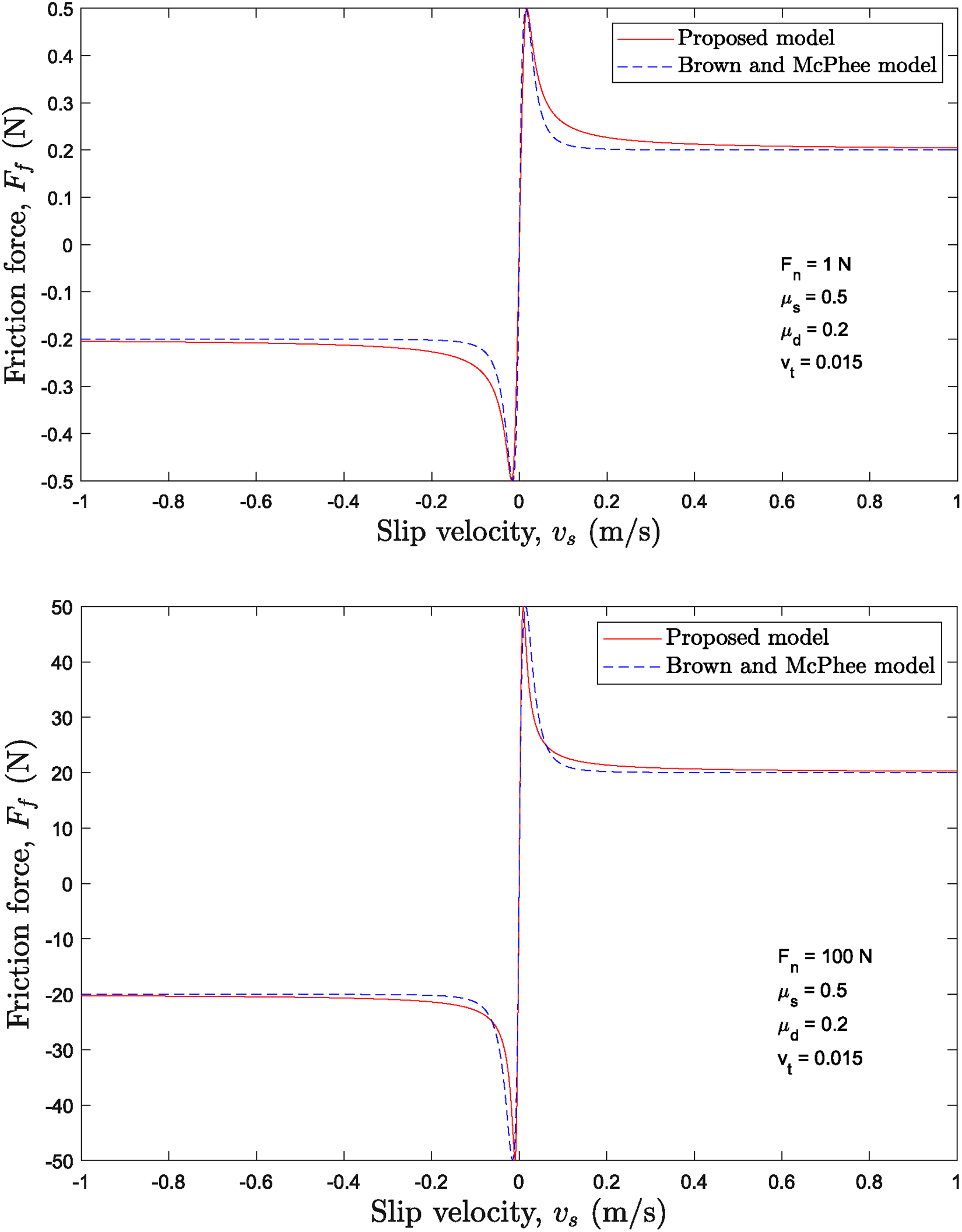
The comparison of friction force profiles against slip velocity.
Hence, it is established, that the proposed friction model behaves similar to the state-of-the-art friction model. This leads to the next section, wherein the proposed model is applied to a benchmark study to demonstrate the applicability of the proposed model.
Validation of proposed model through Rabinowicz’s stick-slip experiment
Figure 2 shows the stick-slip experimental set-up. This benchmark test was used by Brown and McPhee to compare their model against Andersson’s and Hollars’ models. Hence, this simulation study was carried out to compare results of the proposed friction model against Brown and McPhee’s model. A rigid body of mass

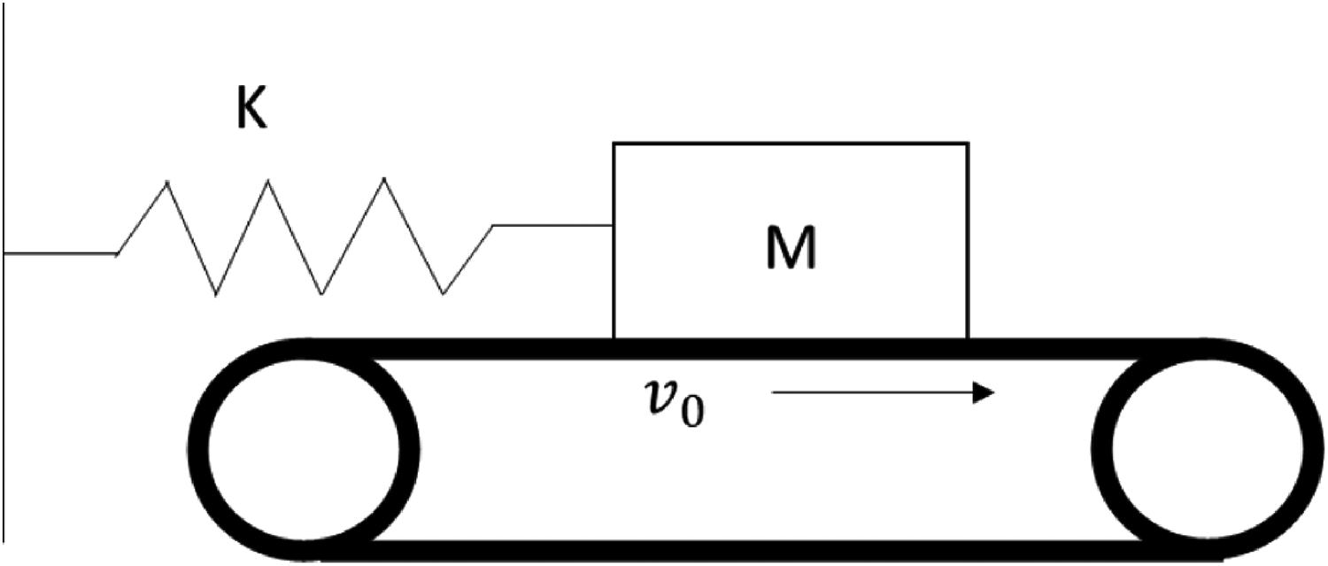
Rabinowicz’s stick-slip experimental setup.
Stick-slip experiment data.
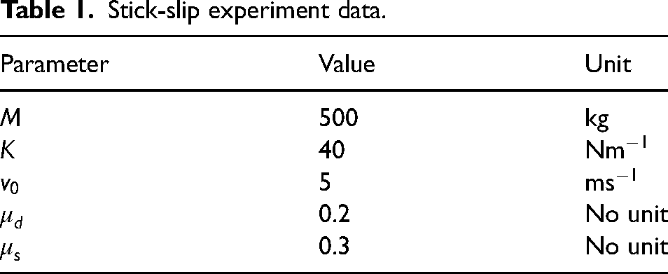
Figure 3 compares the results obtained with the proposed friction model and the Brown and McPhee model on the key dynamic components of the system: position, velocity, and acceleration of the mass. It is concluded from the sudden drops in the acceleration curve that stiction was captured by both models. The transition velocity for the Brown and McPhee model was kept at 15
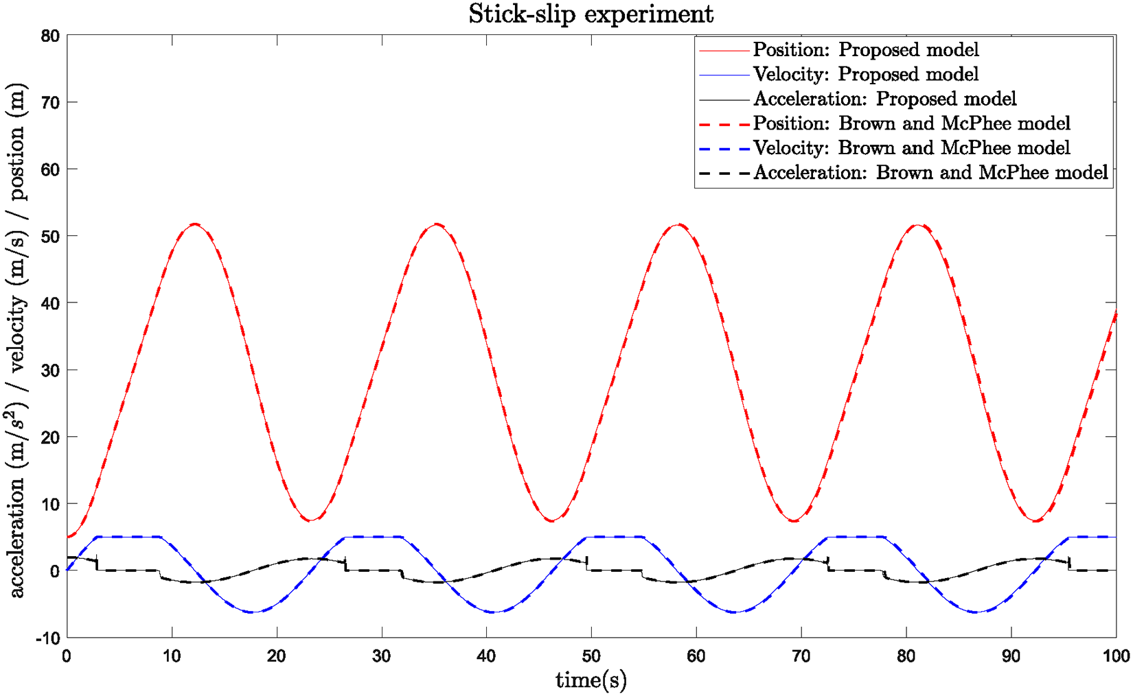
The comparison of position, velocity, and acceleration.
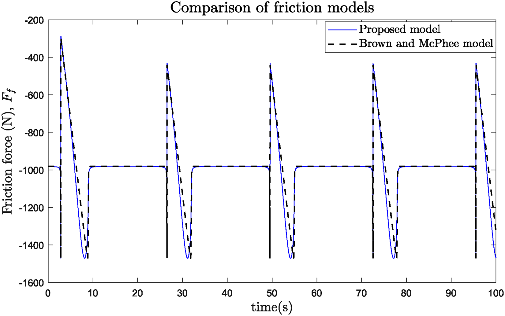
The comparison of friction force.
Root mean squared errors (RMSEs) of dynamic parameters.
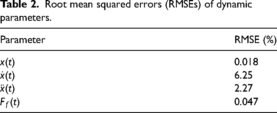
Since the system’s dynamic characteristics (position, velocity, and acceleration) almost overlap each other respectively, it can be concluded that both models perform equally well for this case study. However, such a comparison is incomplete, as in this experiment the normal contact force between the block and the belt does not change with time. Hence, case studies have been performed by applying the proposed friction model to multibody systems where the contact normal forces are time dependent, as discussed in the following section.
Multibody dynamic system formulation
The multibody dynamic systems considered in this study are made of rigid links constrained by joints. Such constrained dynamic systems are usually formulated using index 3, index 2, or index 1 DAEs, however, these DAE formulations consider only one of the position, velocity, or acceleration constraints, respectively. 9 Haug 10 proved that the index 0 tangent space approach captures the highly nonlinear nature of constrained multibody dynamic systems and exhibits better error control with all the dynamic parameters after integration. This is because it includes constraints on position, velocity, as well as acceleration. Hence, the case studies were modeled using this approach.
Formulation of the tangent space index 0 DAE
Consider an orthonormal inertial reference frame
For any generalized coordinates, 
The Jacobian of the constraint manifold, 


Multibody system case studies
In this section, two multibody dynamic systems that were formulated using index 0 tangent space DAEs are described. The constraint equations of relevant joints are presented along with the geometric and inertial parameters of both systems.
Spatial four mass system
As shown in Figure 5, the spatial four mass system consists of four point masses represented by
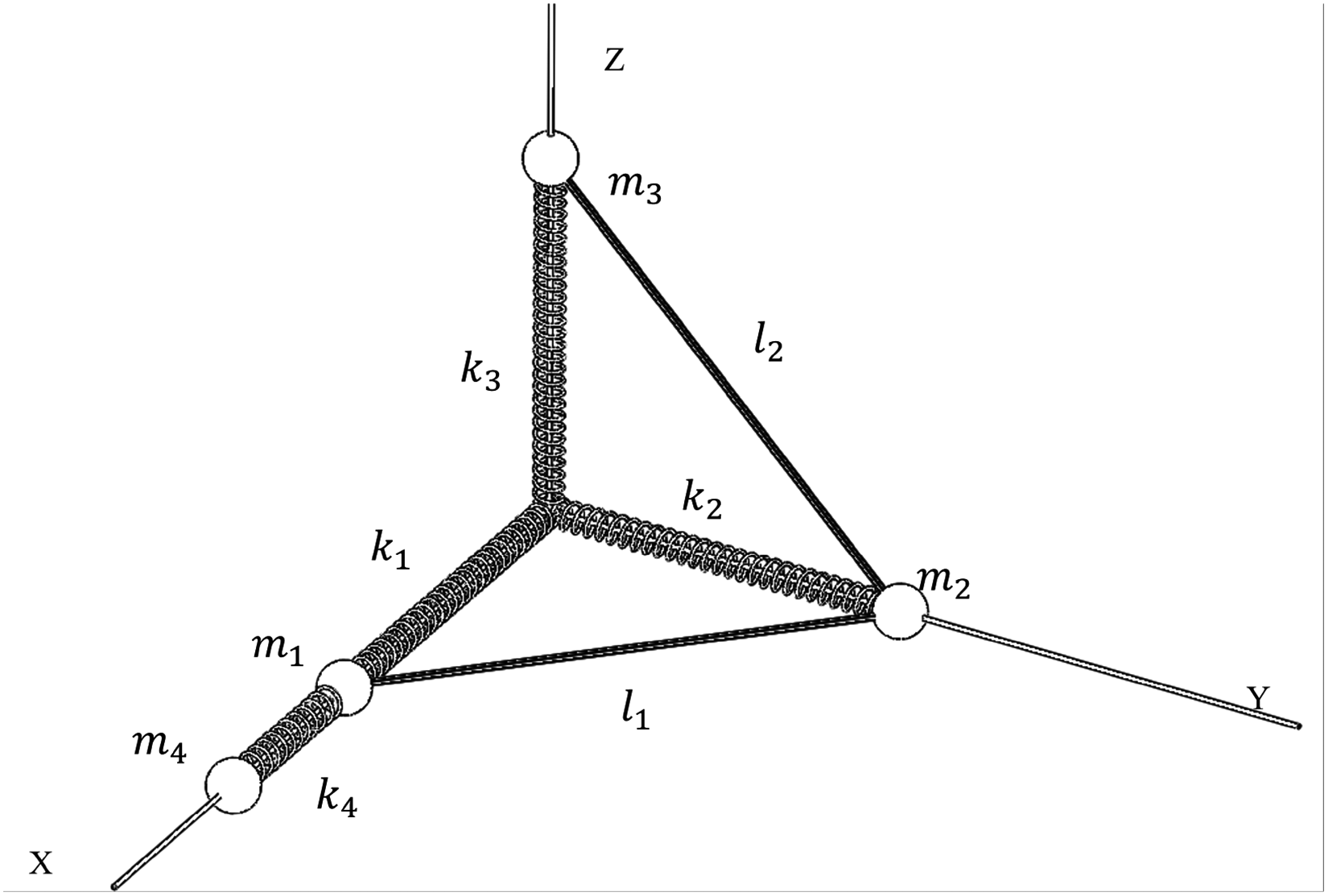
Spatial four-mass system setup.
The masses 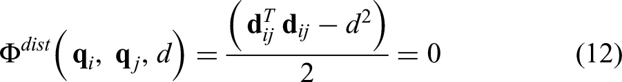

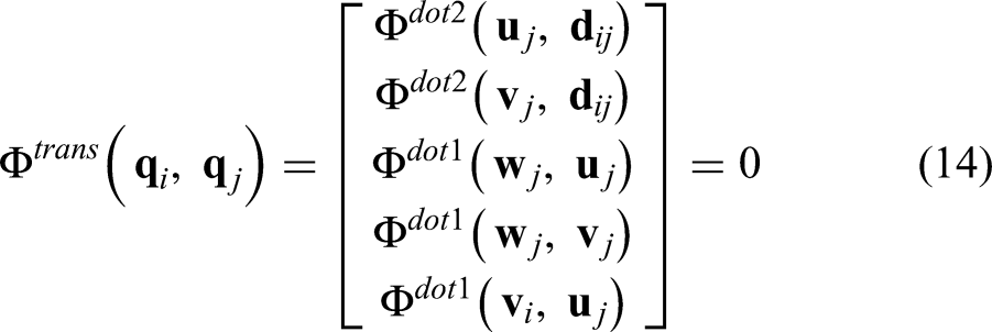


Thus, the system has 22 constraint equations, which results in the system to have only two degrees of freedom. The constraint manifold of the system,
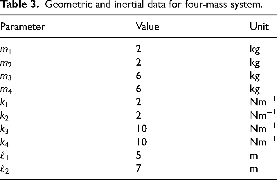
Geometric and inertial data for four-mass system.
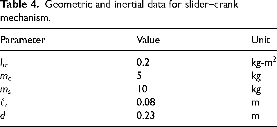
Spatial slider-crank mechanism
As shown in Figure 6, the three-dimensional slider-crank mechanism is composed of a crank, massless connecting rod and slider. The mass and the inertia of the crank about its rotational axis are given by
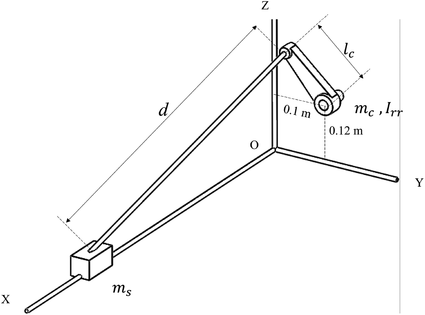
Spatial slider–crank mechanism.
The system has two bodies whose generalized coordinates are given by 
Thus, the system has 11 constraint equations, which results in the system to have only one degree of freedom. The constraint manifold of the system,
Geometric and inertial data for slider–crank mechanism.
The two case studies discussed in this section were simulated using numerical integration. The observations are discussed in detail in the next section.
Analysis and inferences
Anaslysis of the proposed friction model
The Coulomb’s friction model is a nonlinear function with discontinuities. In reality, the highly nonlinear nature of friction arises due to complex phenomena observed at a molecular level, 21 such as surface asperities, material properties, and temperature. However, modeling such phenomena for multibody dynamics and control applications is exceptionally challenging. The question then arises, how to use available information to model friction as close to accurate as possible while meeting requirements for dynamic simulations and controls? The work reviewed, as described in the Introduction section delineated approaches that attempted to remove the discontinuity, yet capturing the nonlinearity using independent quantities, such as slip velocity and coefficient of friction and introducing empirical or manually tunable parameters like transition velocity.
This leads to the next question, which is how to model friction with tunable parameters that do not have to be guessed but that can be obtained by using available information? The proposed model is able to circumvent the issue of having to guess such tunable or empirical parameters by using available information.
This is achieved by computing the tunable parameters using all available information, that is the magnitude of the normal reaction force and the surface properties, such as the static and the dynamic friction coefficients along with the slip velocity. The sine and inverse tangent function in equation (3) capture the nonlinearity while also maintaining
Investigation into the proposed friction model parameters
To understand the effect of each parameter on the friction force model, simulations were performed by varying the query parameter while maintaining other parameters constant.
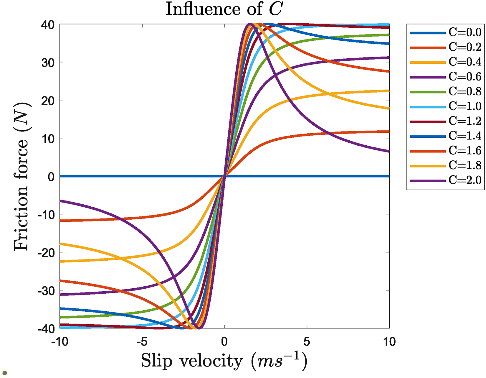
The terms are analogous to Pacejka’s tire model. 22 The parameter C is the “shape factor.” It can be seen in Figure 7 that when C is set to 0, the curve remains a flat horizontal line, indicating there is no friction force. Hence, there is no curvature to the profile, however, as the value of C is increased from 0 to 2, it is seen that curve resembles a negative hyperbolic tangent function until C = 1 and then begins to show a profile as one would expect in a friction force curve against slip velocity. Further, it is seen that, when C is increased beyond 1.4, the peaks become sharper. Since, C controls the shape of the friction force plot, this is a key parameter.
Influence of
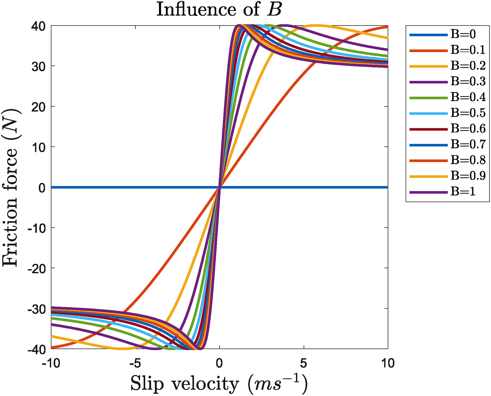
Next, we study the influence of parameter B. The values of B are changed from 0 to 1 as shown in Figure 8. It can be seen that, at B = 0, a flat horizontal line is obtained for the friction force. At B = 0.1 the slope changes but with minimum curvature. Beyond 0.3, the profile remains almost the same however, the negative gradient at zero slip velocity begins to increase. This influences the stiffness of the curve and hence it is termed as the “stiffness factor.”
Influence of
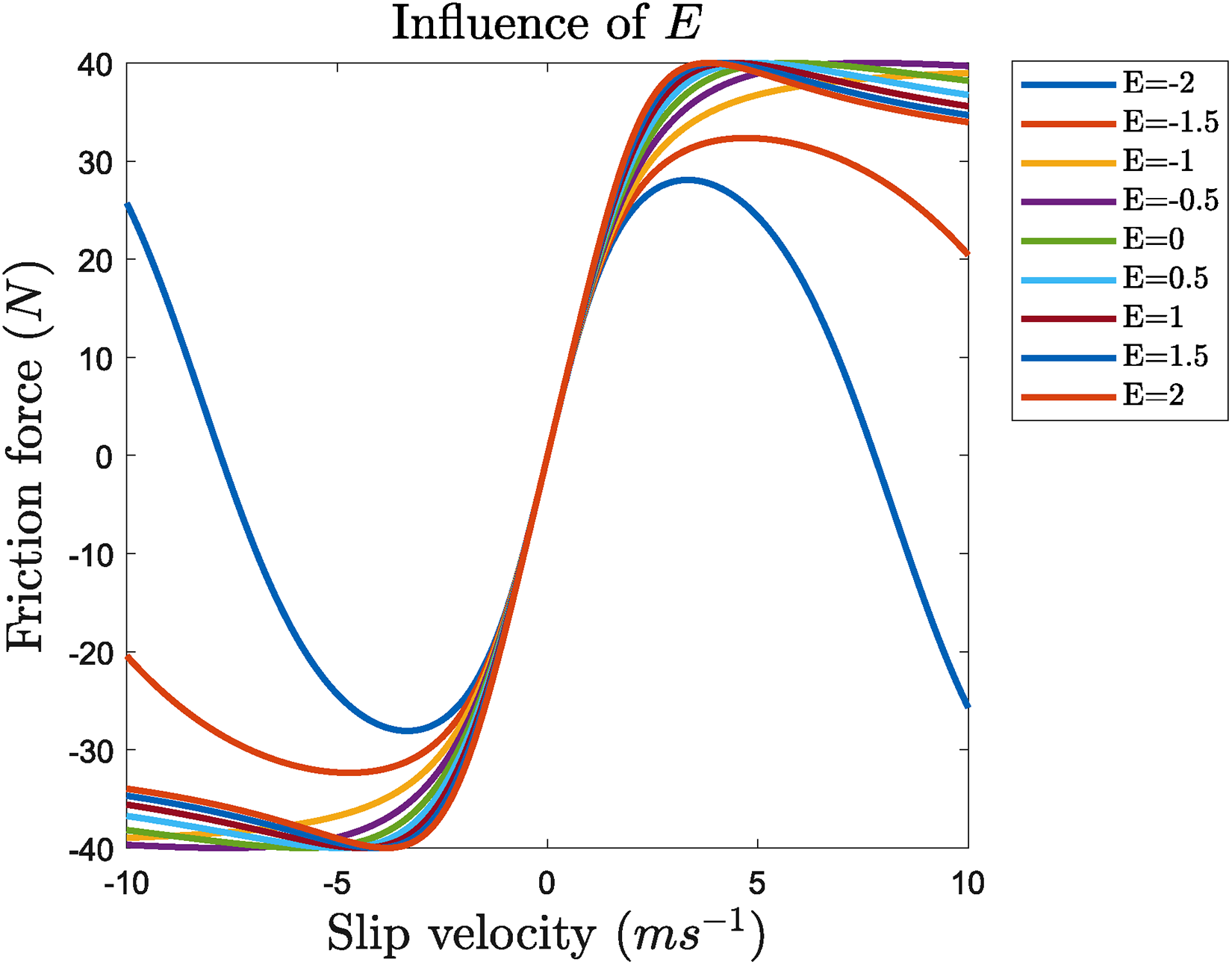
The effect of parameter E on the friction force is presented in Figure 9. It can be seen that for values of E > 0.5, the friction force profile begins to show a sinusoidal behavior, but for values of E < 0.5, the friction force profile is what is as expected. This parameter thus controls the curvature of the friction curve and hence it is known as the “curvature factor.”
Influence of
From the analyses of the three contributing parameters, it can be seen that the choice of C has the strongest influence on the magnitude of the friction. As a consequence, the closer
An investigation into the effect of
The parameter 
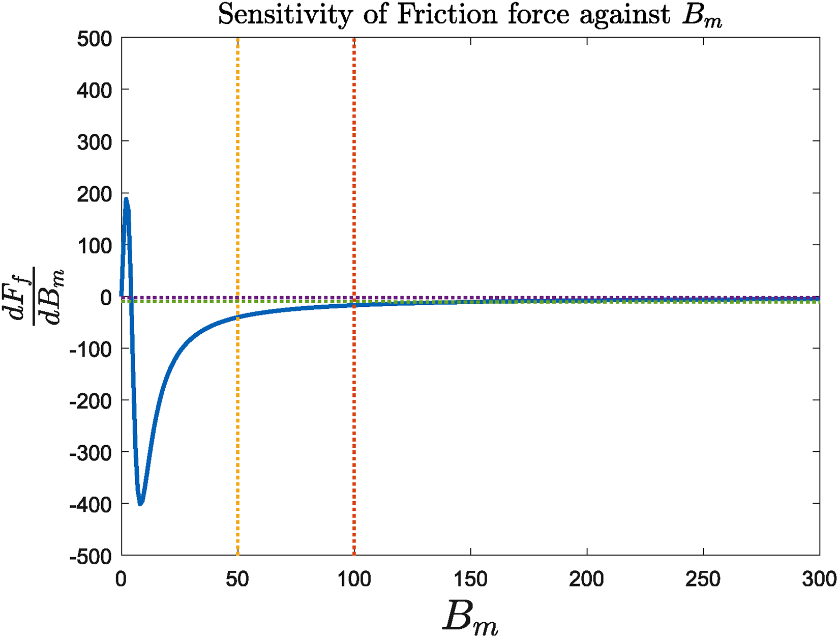
Sensitivity of friction force to
Alongside the information we gather from bristle deflection-based models,
13
the contact surfaces A and B sliding with relative slip velocity
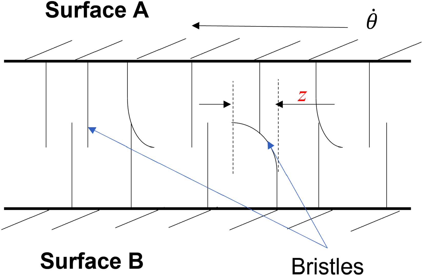
Bristle deflection model.
Secondly, the difference between the static and dynamic coefficients of friction reflects the structural property of individual bristles. A large difference in the coefficients of friction assumes a brittle structure of the bristle. This means, that a large difference in friction coefficients makes the transition faster from static to dynamic regimes as brittle bristles are more prone to fail in shear. However, a small difference in coefficients of friction corresponds to a more ductile structure of bristles and it allows for a slower transition from static to the dynamic regime as bristles go through elastic bending by displacement
Based on the aforementioned inferences, it was deemed necessary to develop a function that evaluates
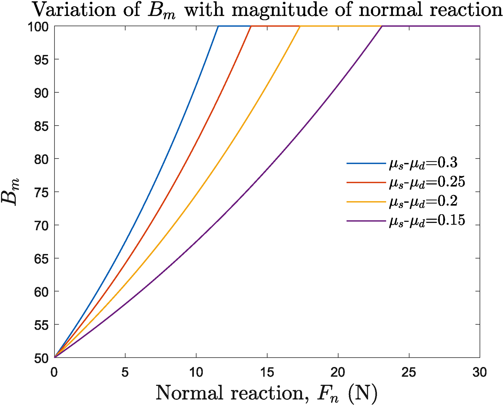
Variation of
Case study simulation results
Spatial four-mass system
This section illustrates the simulation results of the spatial four-mass system case study. For the entirety of the simulation, the joint constraints were not violated and is quantified by the norm of the constraint,
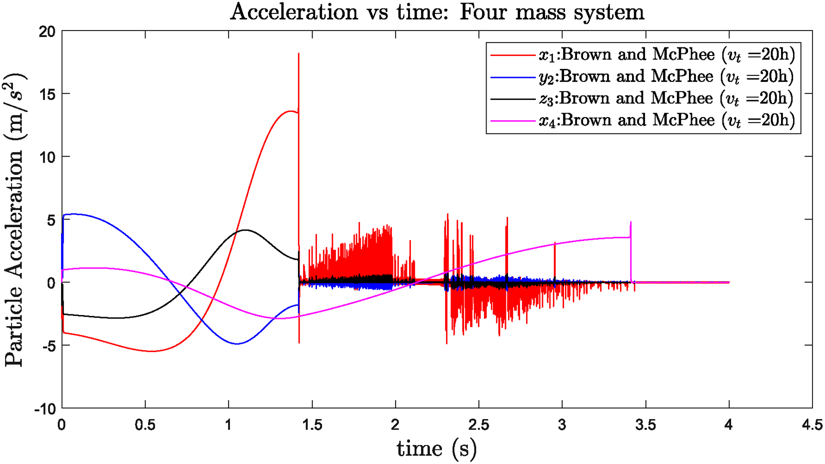
Acceleration versus time: Brown and McPhee model,
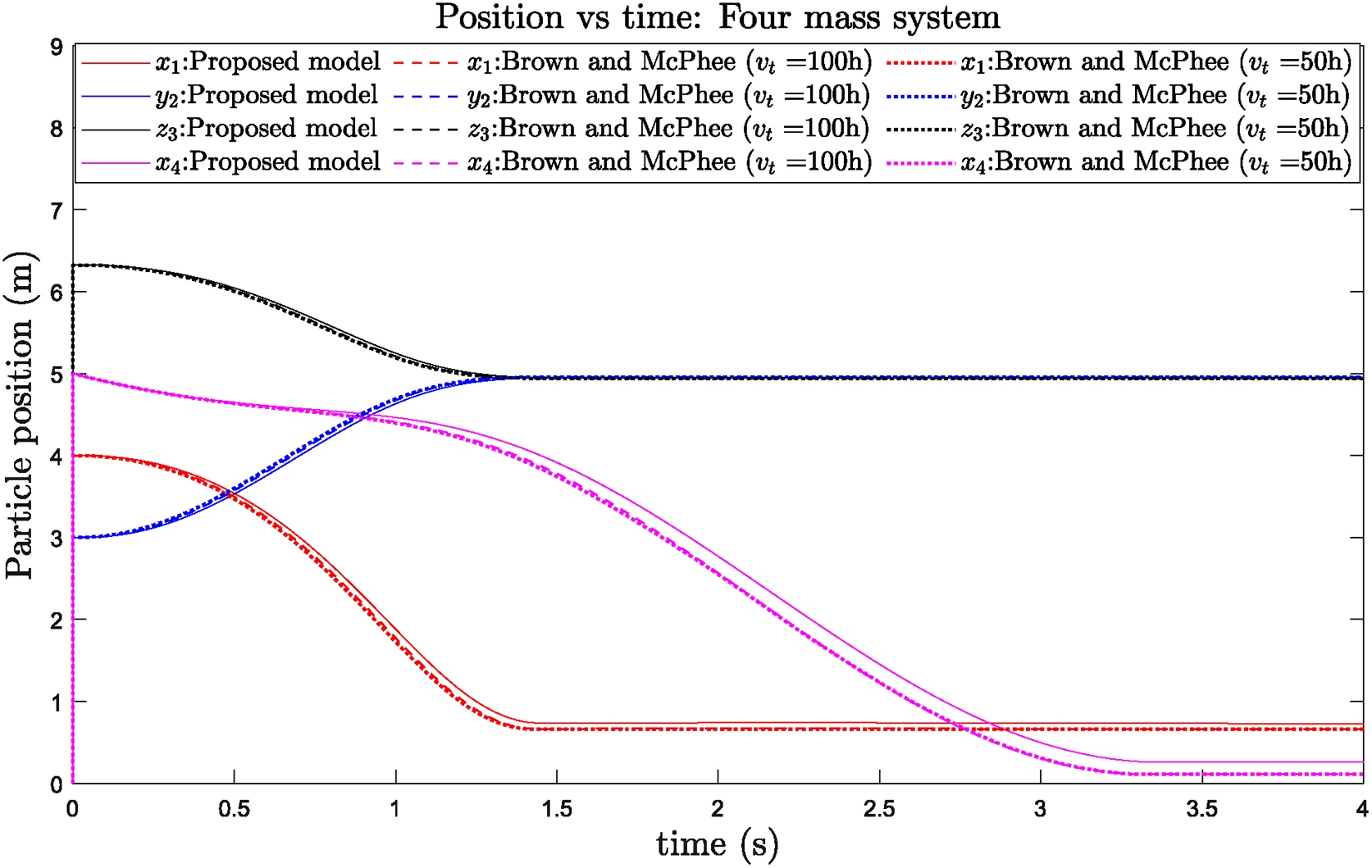
Position versus time: four-mass system.
To fathom further into the sensitivity of the transitional velocity in the Brown and McPhee model, the value for
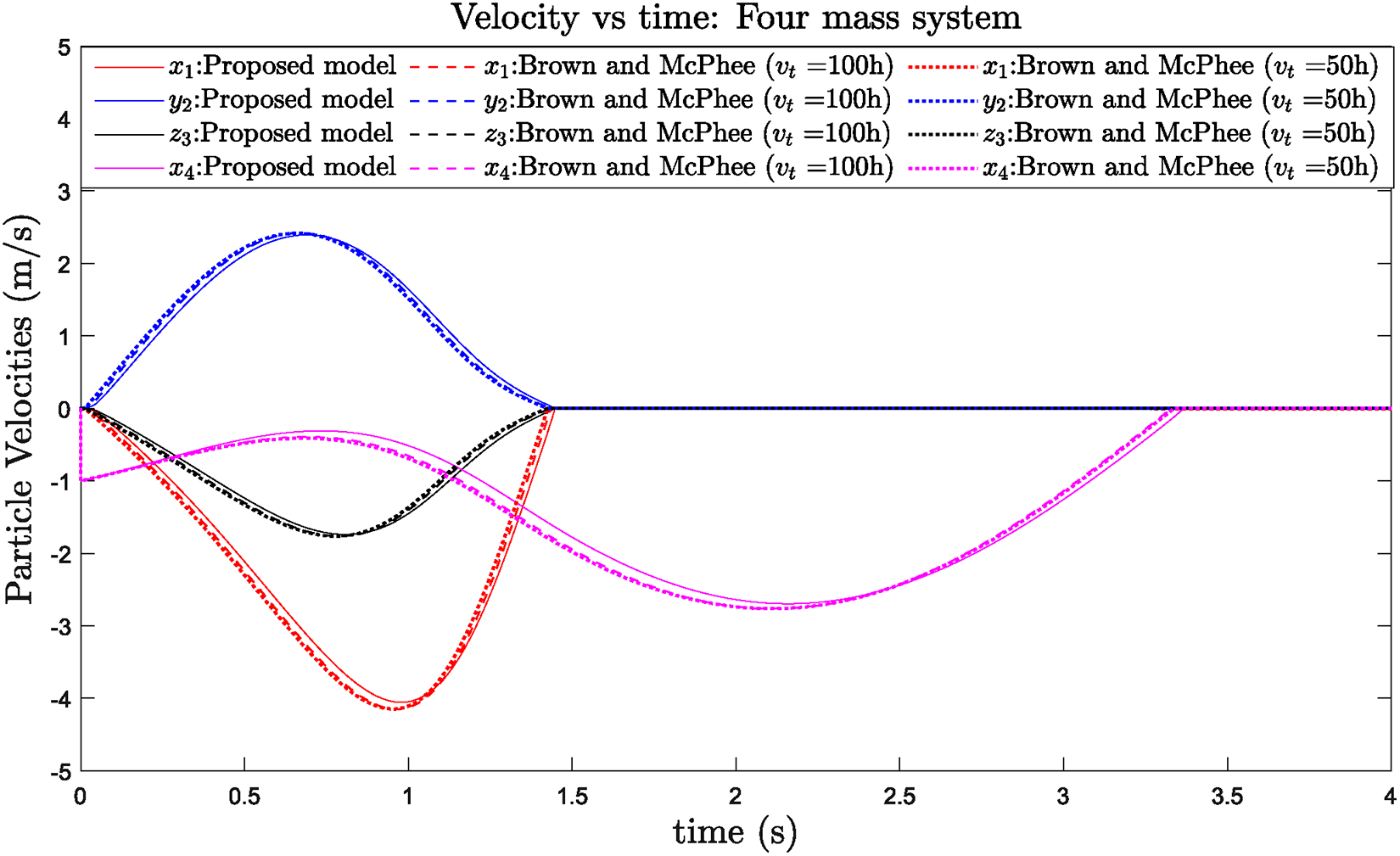
Velocity versus time: four-mass system.
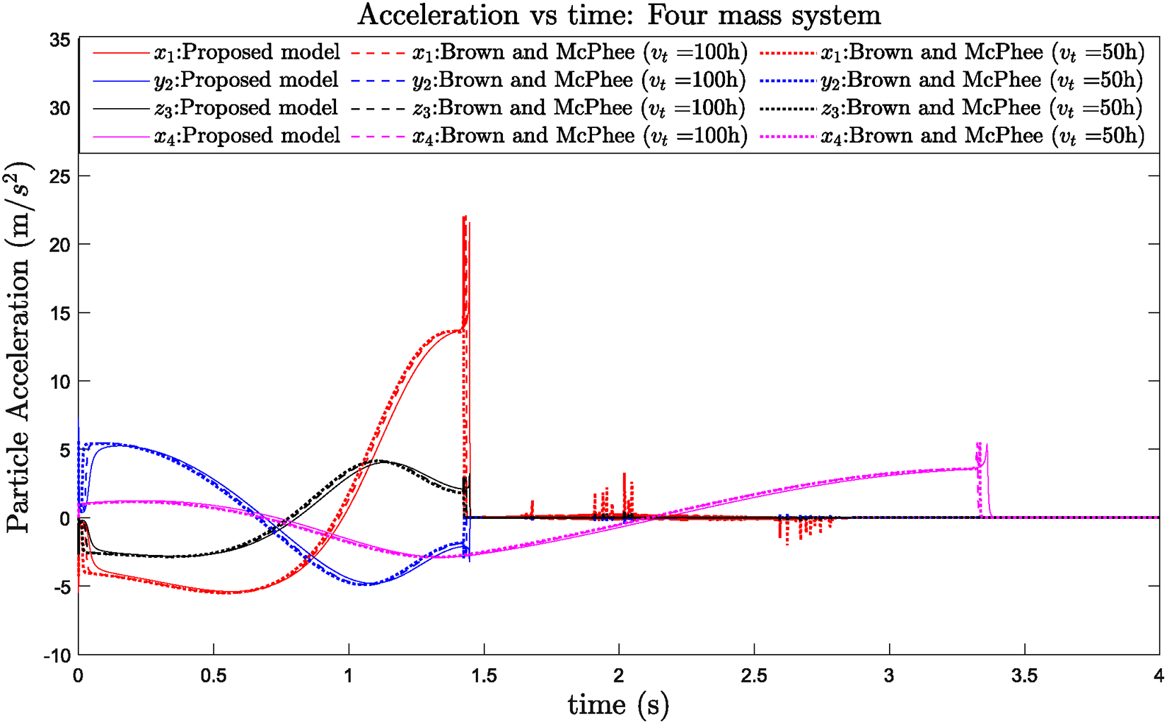
Acceleration versus time: four-mass system.
At
As can be observed from the acceleration plots, the proposed model inherently possesses the capacity to tune the key parameters automatically by taking into account all the information about the forces acting on the body. Because of this inherent characteristic, it provides smooth signals irrespective of the choice of input parameters. This ability could be useful for implementing control systems into the systems with dry friction. The modern state-space control systems employ a number of mechanisms to generate smooth signals, such as anti-aliasing filters and low-pass filters. 23 Especially, in the multi-input and multi-output (MIMO) control systems applications, the number of signal processing devices to employ is directly correlated to the number of signals. It could be a cost effective measure in such cases if the dynamic signals can be smoothened out naturally.
Spatial slider–crank mechanism
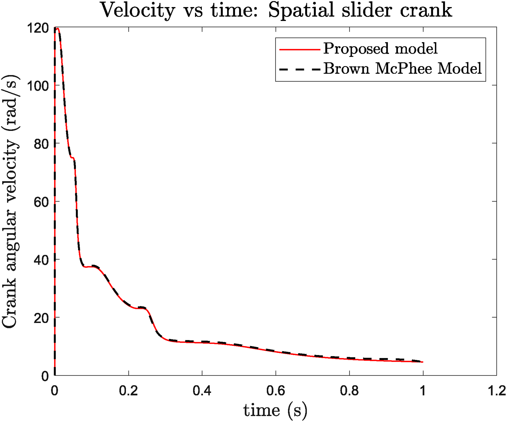
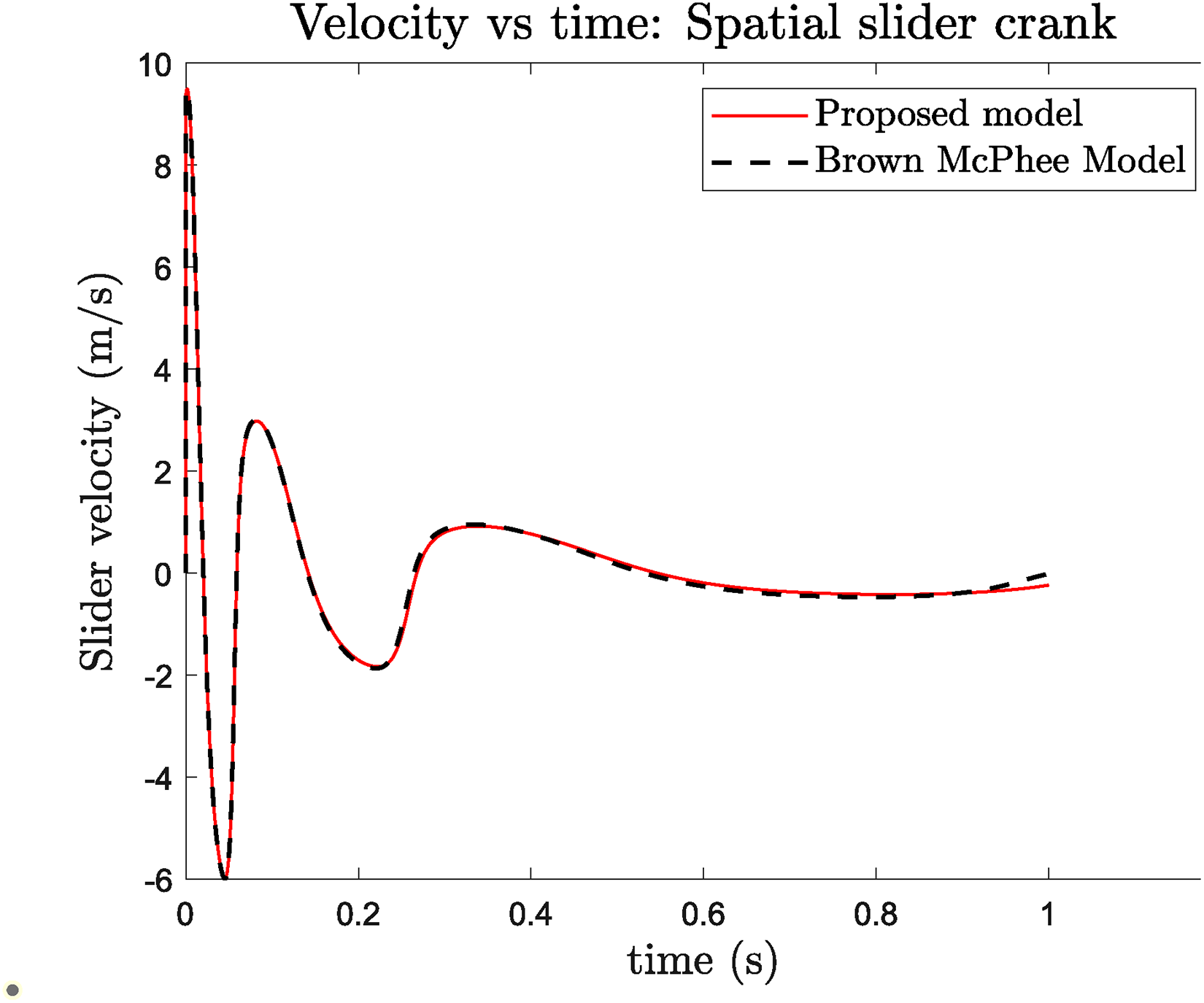
For crank and slider, respectively, Figures 17 and 18 show the accelerations, and Figures 19 and 20 show the velocities. Figure 21 shows the position of slider against time.
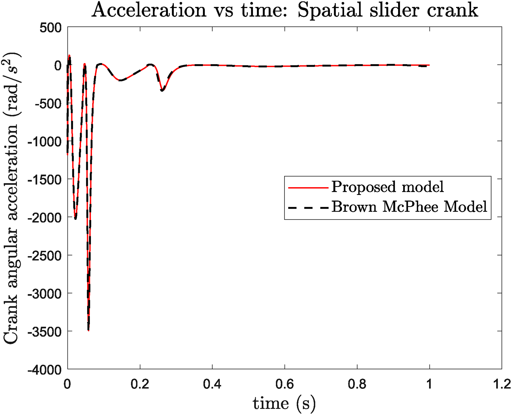
Crank acceleration against time.
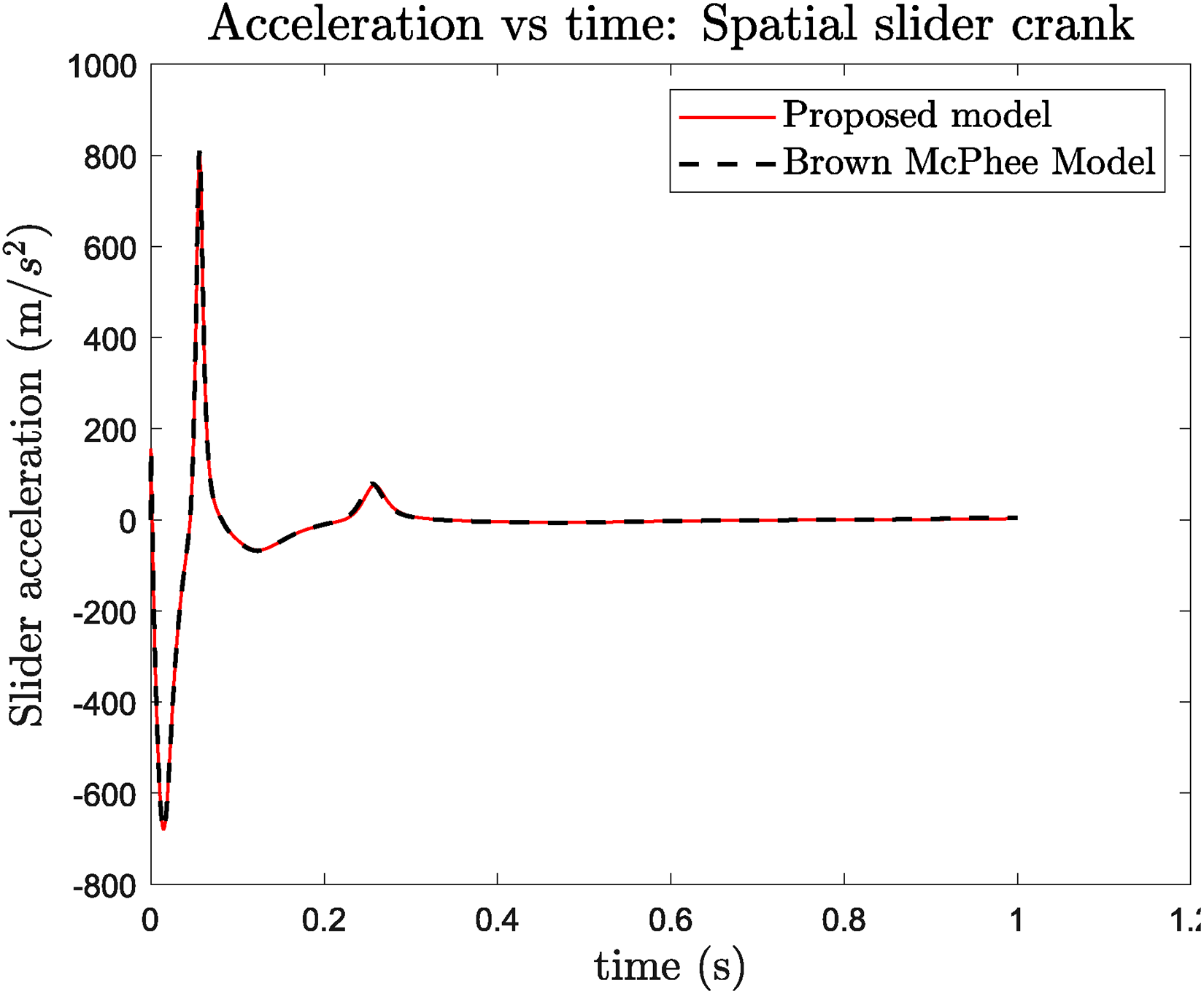
Slider acceleration against time.
Slider velocity against time.
Crank velocity against time.
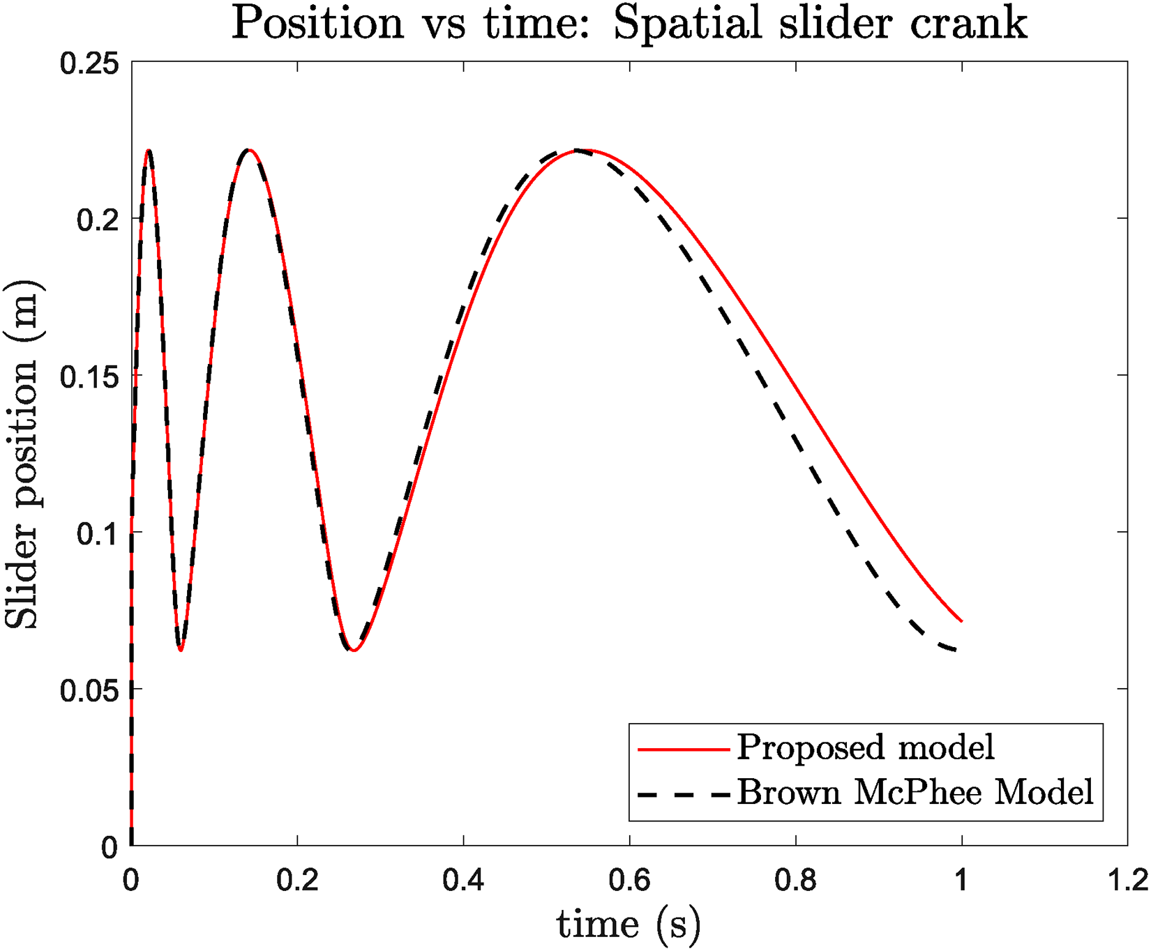
Slider position against time.
As in the previous case study, the joint constraints were not violated and is quantified by the norm of the constraint,
Unlike the spatial four-mass system, no jittery behavior was observed in the acceleration plot. The acceleration and velocity profiles are smooth, and it can be seen that they are very similar, overlapping almost completely. It is, however, observed that after
Conclusions
To summarize, a novel friction model which possesses continuity and differentiability. The proposed friction model has been studied critically for the effect of each of its parameters. The proposed model brings novelty in the terms that, unlike its contemporary friction models, the proposed model does not depend on any empirical parameter such as transition velocity. This makes this model very useful for simulating large-scale multibody systems while considering all the major aspects of friction phenomena. Further, it has the inherent property to tune its parameters such that the produced signals are smooth in nature. This characteristic of the proposed model could prove vital for control system applications where smooth signals are preferred to save costs on anti-aliasing and low-pass filters. The theoretical and conceptual reasoning for the criteria and algorithms to select the model-dependent parameters have been described in detail. The proposed friction model was simulated for the Benchmark Rabinowicz’s stick-slip experiment, which validated the potential for the proposed friction model to be used in the simulation of dynamical systems. The performance of the proposed model was also compared to the state-of-the-art Brown and McPhee’s friction model and it was shown that both models are in agreement. The applicability of the proposed friction model was then demonstrated by simulating two multibody dynamic systems. The index-0 tangent space DAE formulation method was adopted for developing equations of motion of the spatial four-mass system and of the spatial slider–crank system which incorporated into the friction force models. It was concluded that the choice of the transitional velocity Acceleration, could either be an output from a sensor or just a state-space variable in the modern control systems. To deal with multiple jittery signals, the modern control systems often use low-pass filters and anti-aliasing devices. In such control systems where every signal needs to be filtered with a device of appropriate band-width and Nyquist frequency, a lot of cost could be saved by having jitter-free signals. From the simulation results incorporating the proposed friction model, it was seen that similar results can be indeed achieved, while no jittery behavior can be seen. This was accomplished by eliminating the need for manually tunable parameters and instead using parameters that use available information from the system. The algorithm has been explained as to how it inherently accounts for the shape and stiffness factors thus adapting to slight changes in normal force and slip velocity. Hence, the proposed friction model can be used for multibody dynamic system applications. The future scope of this work includes implementing the model into designing control systems and testing this model against one that includes bristle deflection theory, such as the LuGre and Gonthier’s model. Further improvements that can be carried out on the proposed model is to include the viscous friction regime.
Footnotes
Acknowledgements
This research did not receive any specific grant from funding agencies in the public, commercial, or not-for-profit sectors. The authors express their special gratitude to Dr. Edward J. Haug for sharing his insights through his benign mentorship.
Declaration of Conflicting Interests
The author(s) declared no potential conflicts of interest with respect to the research, authorship, and/or publication of this article.
Funding
The author(s) disclosed receipt of the following financial support for the research, authorship, and/or publication of this article.