Integrating climate projections with Gaussian processes for structural anomaly detection via cointegration

Abstract

Ensuring the long-term safety and durability of civil infrastructure increasingly depends on data-driven structural health monitoring systems capable of objectively tracking changes in structural performance. However, their reliability is undermined by the evolving environmental conditions associated with climate change. Variations in temperature and other environmental factors can modify the dynamic response of a target structure, producing apparent changes in damage-sensitive features that may be misinterpreted as degradation. Therefore, distinguishing environmental influences from genuine structural deterioration is essential for a reliable assessment. This study presents an integrated framework for resilient structural monitoring that separates climate-induced variability from damage effects. The methodology combines automated operational modal analysis with Gaussian process regression to model the nonlinear dependence of natural frequencies on temperature and quantify uncertainty. Climate projections from the CH2018 model under Representative Concentration Pathway scenarios are incorporated to forecast the long-term evolution of modal properties. The approach is demonstrated on the case study of the Chillon Viaduct in Switzerland, where continuous monitoring revealed a consistent reduction in natural frequencies with increasing temperature, reflecting temperature-dependent material, revealing a consistent reduction in natural frequencies with increasing temperature, reflecting a combination of thermally driven mechanisms, including material property changes and structural boundary variations. Sparse Gaussian process models enabled efficient long-term forecasting of frequency variations while maintaining predictive accuracy. Cointegration analysis was used to remove temperature-driven trends, isolating residuals sensitive to structural damage. Simulated progressive-damage scenarios confirmed the method’s capacity to detect incipient deterioration under varying environmental conditions. Overall, this work establishes a robust and generalizable framework that integrates modal analysis, probabilistic modeling, and climate projections to improve the resilience, interpretability, and long-term applicability of structural monitoring systems.

1. Introduction

Structural Health Monitoring (SHM) in general, and vibration-based SHM in particular, are key research fields in civil and structural engineering, with the aim of developing and implementing strategies to ensure the safety, durability, and efficiency of infrastructures throughout their life cycle.^1,2 In an era of complex structures and rapidly changing environmental conditions, vibration-based SHM acts as a proactive system for early damage detection, structural performance assessment, and maintenance planning. This field combines advanced sensor technologies, data analysis algorithms, and predictive models to transform raw data into critical information for real-time engineering decisions.^3–5 Alongside vibration-based and physics-informed monitoring strategies, machine-learning-based approaches are becoming increasingly important in intelligent condition monitoring, including classification-based diagnosis, pattern recognition, and data-fusion strategies for industrial and mechanical systems.^6–8

The choice and deployment of a specific (vibration-based or not) SHM strategy is usually driven by the type of structure, the required performance, and the monitoring goal, which in turn dictate the temporal scope and nature of the assessment. An increasingly adopted paradigm is continuous monitoring using permanently installed sensor systems, enabling long-term performance assessment and maintenance planning. Among the various techniques for continuous monitoring, vibration-based SHM is among the most widely researched and applied, ⁹ showing promising results in different infrastructure monitoring applications.^10–12 This method is based on the assumption that the dynamic response of a structure, measured under ambient or operational vibrations, contains vital information about its physical condition. Variations in identified dynamic characteristics can therefore be systematically linked to the initiation and progression of structural damage. To capture these variations, damage-sensitive features are extracted from the measured response data. Global features, such as natural frequencies and damping ratios, reflect changes in the overall mass, stiffness, and boundary conditions of the system, ¹³ with changes in these quantities often serving as early indicators of potential damage. ⁵ In contrast, local or spatially dependent features, including mode shapes, modal curvature, and flexibility-based metrics, provide more detailed information on the probable location and, in some cases, the severity of the damage. ¹³

Despite significant advances in vibration-based SHM, these methods often face limitations in real-world deployment. One primary concern is the sensitivity of damage-sensitive features to operational and environmental factors.^14,15 This variability is a major challenge because it can mask the subtle signatures of true structural degradation or, conversely, trigger false alarms. ¹⁶

Several studies highlight that temperature changes can significantly influence observed variations in modal properties, making it challenging to distinguish between environmental influences and actual structural degradation. For example, a recent study on the Italian steel truss girder bridge Ostiglia-Revere et al. ¹⁷ found that natural frequencies vary with ambient temperature, indicating that temperature must be considered when interpreting monitoring data. In another investigation of short-span concrete bridges in Korea, Cho et al. ¹⁸ observed that natural frequencies tend to decrease as temperature increases, and that different types of bridges (slab versus rigid frame, with or without elastomeric bearings) show different sensitivity to temperature variation. Similar findings are reported in a technical study on several bridges in the United States, where temperature was shown to significantly affect natural frequencies in a non-linear manner, emphasizing the need for temperature compensation in vibration-based SHM applications. Taken together, these results show that temperature fluctuations can induce substantial variations in modal parameters, making it difficult to distinguish between environmental effects and actual structural degradation. This overlap compromises the reliability of monitoring systems, particularly in the context of climate change. ¹⁹

Existing research widely acknowledges the temperature dependence of frequency-based features and the challenge of separating those effects from damage accumulation. To address this issue, the research community has pursued two distinct strategies: (i) identifying damage-sensitive features that are inherently insensitive to environmental and operational variations (EOV), and (ii) developing models to remove this influence from the parameters themselves. The first strategy, while ideal, is more challenging and remains an active area of research. ²⁰ The second strategy is more common and has been applied more broadly. This approach acknowledges the dependency of features on EOVs and applies data-driven models to isolate and mitigate environmental effects. The goal is to establish a healthy baseline that accounts for regular environmental cycles, so that deviations from it are more likely to indicate damage. A variety of methods have been developed for this purpose. Some researchers use statistical models, such as ARIMA, to account for time-dependent data and filter out environmental influences. ²¹ Others rely on linear approaches to remove environmental effects ²² or on multivariate statistical techniques, such as Principal Component Analysis (PCA), to decouple structural damage from environmental variability. ²³ Recent work has also demonstrated unsupervised real-time damage detection that decouples EOVs from damage cases using PCA in combination with cepstral characteristics. ²⁴ Factor analysis and spatial filtering have been proposed as additional means of modeling and removing environmental influences from vibration-based SHM data. ²⁵ Recent reviews further synthesize these developments and provide a comprehensive overview of data-driven strategies to eliminate environmental effects. ²⁶

Among this second family of solutions, methods such as cointegration have shown particular promise by identifying long-term relationships between non-stationary variables and filtering environmental trends to reveal damage-related deviations. Studies by Cross et al. ²⁷ and Zhang et al. ²⁸ demonstrated the effectiveness of cointegration in removing temperature effects from vibration-based SHM data. Coletta et al. ²⁹ applied cointegration to historical building monitoring data, successfully isolating the effects of seasonal temperature and humidity. Similarly, Kuai et al. ³⁰ expanded the application of nonlinear cointegration to offshore platforms, utilizing Support Vector and Relevance Vector Machines to compensate for complex wind and wave loading conditions. More recently, the traditional linear formulation of cointegration has been extended to incorporate nonlinear regressors, enabling the capture of more complex relationships between environmental variables and structural responses. In this context, Gaussian Process Regression (GPR) has been proposed as a flexible probabilistic tool, capable of modeling nonlinear environmental dependencies while also quantifying predictive uncertainty. Shi et al. ³¹ embedded GPR within the Engle–Granger framework and applied it to the monitoring data from the Z24 Bridge, showing that the method can effectively remove environmental and operational effects while providing probabilistic confidence bounds that enhance the robustness of vibration-based SHM.

In addition to probabilistic approaches, recent advances in engineering decision-making have highlighted the value of fuzzy multi-criteria decision models for representing epistemic uncertainty, expert hesitation, and incomplete or conflicting information. For example, T-spherical dual hesitant fuzzy sets have been proposed to support decision-making when multiple uncertain indicators must be combined into interpretable engineering assessments. ³² Related fuzzy-rough and fuzzy multi-criteria models have also been developed for complex engineering decision problems where quantitative predictions must be integrated with expert judgment and scenario-dependent uncertainty.^33,34 In the context of climate-resilient SHM, such approaches are complementary to probabilistic tools such as Gaussian Process Regression. While GPR provides uncertainty-aware predictions of modal properties under changing environmental conditions, fuzzy decision models could support the downstream interpretation of residual-based indicators by translating probabilistic outputs, climate-scenario uncertainty, and sensor-confidence information into graded maintenance-oriented risk categories.

Most existing studies addressing environmental effects in vibration-based SHM rely on correlating modal properties with observed environmental variables, typically through regression or statistical filtering. Although such approaches have proven valuable for understanding short-term variability, they remain fundamentally calibrated on historical environmental regimes and therefore become less reliable when environmental drivers evolve beyond their training domain. This limitation is particularly critical under ongoing climate change, where rising baseline temperatures and increasingly frequent extreme events are shifting operational regimes outside historical norms. Data-driven models that assume environmental stationarity thus face a severe extrapolation problem, producing unreliable predictions when applied to unseen climate conditions. This challenge is different from many recent intelligent monitoring problems in manufacturing and mechanical systems, where machine-learning classification or diagnostic-fusion strategies are often used to identify localized or process-specific fault patterns, such as machining instabilities or rotating-machinery faults.^7,8 In those settings, the monitoring task is commonly formulated as classification or evidence fusion. In contrast, climate-adaptive SHM of civil infrastructure must address slow, non-stationary environmental baselines that evolve over years or decades and may induce modal-property variations comparable to those caused by structural deterioration. The central challenge is therefore no longer only to remove present environmental variability, but also to preserve damage sensitivity when the environmental baseline itself changes over time.^15,19 Accordingly, the proposed framework emphasizes probabilistic environmental modeling, climate-scenario propagation, and cointegration-based residual analysis to preserve damage sensitivity under non-stationary environmental conditions, rather than relying on direct classification or diagnostic fusion alone.

A recent milestone in this direction was the work of Figueiredo et al., ¹⁹ who demonstrated that climate change can degrade the long-term reliability of damage detection models trained on historical bridge data. Using machine-learning classifiers applied to the Z24 Bridge, their study showed that increases in mean temperature under future climate scenarios could significantly alter model performance, increasing false-negative rates and challenging the assumption of static environmental baselines. However, that work primarily assessed the vulnerability of existing damage detection models to changing climate conditions, without proposing an uncertainty-aware predictive framework to model, propagate, and compensate for those evolving effects.

The distinctive contribution of this study does not lie in the individual application of its methods, which are well established in their respective domains, but in their integrated use within a single climate-adaptive workflow (Figure 1).

Figure 1.

Workflow of the proposed climate-adaptive SHM framework. Modal features identified from monitoring data are related to temperature through sparse Gaussian Process regression and propagated under future climate scenarios. Residual analysis is then used to distinguish environmentally induced variability from potential damage-sensitive deviations and to determine whether model updating is required.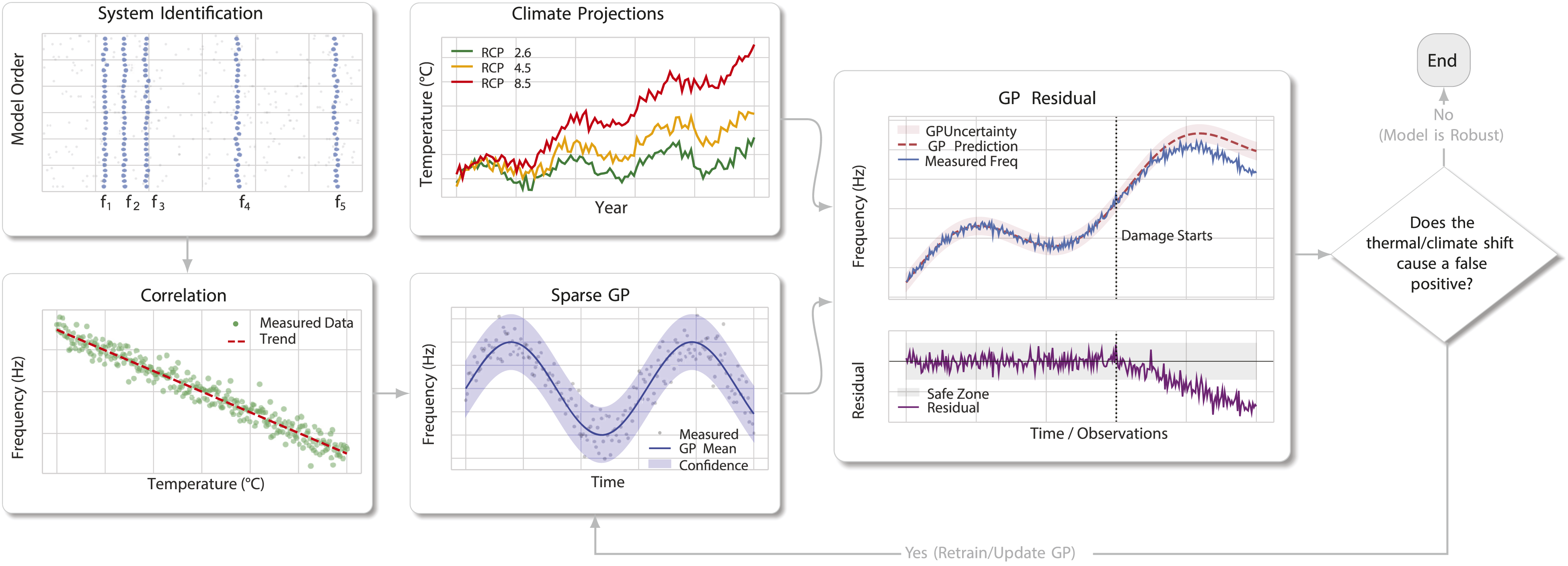

The proposed framework combines: (i) Automated Operational Modal Analysis (AOMA) for continuous feature extraction; (ii) sparse Gaussian Process modeling to capture the nonlinear temperature–frequency relationship while quantifying predictive uncertainty; (iii) climate-projection-informed forecasting to evaluate the long-term evolution of modal properties under RCP scenarios; and (iv) cointegration-based anomaly extraction to recover damage-sensitive residuals under evolving environmental conditions. In this way, environmental variability is not treated merely as a source of noise to be filtered out, but as a quantity that can be explicitly modeled, projected, and normalized within the monitoring process.

Building on this motivation, the present paper introduces a climate-adaptive, data-driven monitoring framework that explicitly couples structural response modeling with climate projections. The framework is validated using continuous vibration data from Switzerland’s Chillon Viaduct, collected since 2017. Automated system identification is first used to extract modal parameters from the monitored response. Sparse GPR is then employed to model the nonlinear dependence of natural frequencies on temperature and to quantify the associated predictive uncertainty. Representative Concentration Pathway (RCP) scenarios from the CH2018 regional climate model are incorporated to propagate these relationships under future environmental conditions. Finally, cointegration analysis is applied to the normalized indicators to isolate residuals that remain sensitive to structural change. By integrating real monitoring data, probabilistic environmental modeling, climate projections, and anomaly-sensitive residual analysis, the proposed methodology establishes a pathway toward predictive, climate-resilient vibration-based SHM, supporting long-term safety, maintenance planning, and adaptation of bridge infrastructure in a warming climate.

In this broader context, the present work can also be viewed as contributing toward the methodological foundations of climate-aware Digital Twin frameworks for civil infrastructure. While the study is positioned here within vibration-based SHM, its novelty lies in showing how continuous monitoring, probabilistic environmental modeling, climate projections, and anomaly-sensitive feature extraction can be integrated within a single workflow. Beyond the specific case study, this contribution is relevant because it addresses a central challenge for both SHM and Digital Twin paradigms: maintaining reliable structural interpretation when environmental baselines evolve over time. In this sense, the proposed framework does not simply compensate for environmental variability but establishes a pathway for embedding climate-adaptive monitoring capabilities into future digital representations of infrastructure systems.

2. Methodology

The proposed approach establishes a resilient vibration-based SHM framework designed to adapt to evolving environmental and operational conditions through four main steps: system identification, regression analysis with uncertainty quantification, evaluation of climate projections, and removal of environmental effects. Although this structure defines the overall methodology, each component can be tailored to the specific application.

The process begins with the characterization of the structure’s dynamic properties using an Automated Operational Modal Analysis (AOMA) to extract natural frequencies and mode shapes from ambient vibration data. To address environmental variability, a Gaussian Process Regression model captures the dependencies between environmental factors and dynamic properties, providing predictive uncertainty estimates. This model is then integrated with future climate projections to forecast long-term structural behavior. Finally, cointegration analysis is applied to isolate true structural changes from environmentally induced variations by exploiting stable long-term relationships among variables.

The following subsections will detail the theoretical foundations, implementation steps, and validation protocols for each step, ensuring the reproducibility and scalability of the framework across diverse infrastructure systems.

The methodology developed in this work can be viewed as a robust, data-driven module designed to support a broader digital-twin architecture. By focusing on the vibration-based SHM-specific problems of environmental normalization and damage-sensitive residual extraction, this module provides the diagnostic foundation upon which a structural Digital Twin can be built.

2.1. System identification

A central objective of vibration-based SHM is to characterize the dynamic behavior of a structure from its measured vibration response. This is often achieved through system identification techniques that extract modal parameters, such as natural frequencies, damping ratios, and mode shapes, that collectively reflect the structure’s physical state and serve as key indicators of its integrity and performance.

For long-term and continuous monitoring, Operational Modal Analysis (OMA) has emerged as the standard approach.^35,36 In contrast to traditional forced-vibration testing, OMA relies exclusively on ambient excitations, thereby enabling non-intrusive, cost-effective monitoring of large-scale civil infrastructure without interrupting normal operation. Within the OMA framework, Stochastic Subspace Identification (SSI) stands out as a robust and widely adopted family of algorithms. ³⁷ The method constructs a state-space representation of the dynamic system from a Hankel matrix of measured vibration data and, from this model, estimates the modal parameters. The physical modes are then typically distinguished from spurious mathematical poles using a stabilization diagram, where they appear consistently across various model orders. ³⁸ The reliability of this identification process is critically dependent on the careful selection of algorithm parameters, particularly the number of block rows in the Hankel matrix and the system order. ³⁹

However, manual interpretation of stabilization diagrams introduces subjectivity and limits scalability in long-term applications. To address this, recent research has advanced automated operational modal analysis, improving the baseline SSI procedure through data-driven parameter selection, clustering, and validation. The development of AOMA can be traced back to classical subspace-based methods, ³⁷ which provided a theoretical foundation for OMA. Later, fully automated operational approaches were introduced, enabling robust identification with minimal user intervention. ⁴⁰ More recently, machine learning techniques have been incorporated to further enhance automation and reliability in the estimation of modal parameters.^41,42

In this work, the automated identification strategy proposed by Mugnaini et al. ⁴¹ is adopted. The procedure begins with a wide SSI analysis performed over a wide range of model orders to generate a dense stabilization diagram that contains all potential poles. The resulting dataset undergoes a multi-stage filtering and validation pipeline designed to progressively isolate the true structural modes. The first stage applies Hard Validation Criteria (HVC) based on physical constraints, such as enforcing positive damping ratios within realistic bounds (typically 0–20%) and ensuring complex-conjugate pole pairs, to eliminate clearly nonphysical results.

Subsequently, Soft Validation Criteria (SVC) are employed to statistically assess the consistency of remaining poles across adjacent model orders. Instead of fixed thresholds, these criteria are inferred from the data by evaluating several comparison parameters derived from eigenvalues, natural frequencies, damping ratios, and mode-shape correlation metrics such as the Modal Assurance Criterion and Mean Phase Deviation. A k-means clustering algorithm is then applied in this multi-dimensional feature space to distinguish stable poles from unstable ones.

The stable poles are further grouped through hierarchical clustering, which combines frequency similarity and mode-shape correlation to form candidate clusters. Densely populated clusters are assumed to represent physical modes, while sparse clusters are considered spurious. A second k-means clustering step automatically separates these two categories. Finally, outlier removal is performed within each physical cluster, and a single representative set of modal parameters is derived for each identified mode using statistical aggregation.

In the final stage of the pipeline, the refined physical clusters are cleaned of any remaining outliers. With the clusters now containing only highly consistent poles, a single representative set of modal parameters is estimated for each identified mode by applying statistical measures.

2.2. Climate projection

Climate models are advanced computational systems that synthesize knowledge from physics, chemistry, biology, and computer science to simulate the Earth’s climate and project its evolution under different socioeconomic scenarios. ⁴³ These projections form a fundamental basis for global assessments, such as those of the Intergovernmental Panel on Climate Change (IPCC), and inform policy decisions and adaptation strategies for infrastructure and societal resilience. ⁴⁴ This report reviews the modern climate modeling workflow, from the physical foundations of Global Climate Models (GCMs) to the derivation of actionable, local-scale insights, highlighting key sources of uncertainty, including unresolved small-scale processes and future development pathways, and outlining how downscaling, bias correction, and ensemble modeling are employed to refine projections and quantify future climate risk.

Global Climate Models (GCMs) operate at the planetary scale, integrating key variables that represent the coupled dynamics of the atmosphere, oceans, land, cryosphere, and biosphere. ⁴⁵ They solve fundamental physical equations to simulate these interactions under varying greenhouse gas emissions, energy use, and policy scenarios, often drawing from Integrated Assessment Models ⁴⁶ that incorporate socioeconomic and technological pathways.

Uncertainty in GCM projections arises from several sources. Internally, it originates from parameterizations of physical, chemical, and biological processes that are incompletely understood or empirically approximated, such as atmospheric convection and ocean heat uptake, which different models treat in distinct ways. Externally, uncertainty is driven by the unpredictability of future greenhouse gas emissions, shaped by evolving economic, political, and social conditions. ⁴⁴ As a result, emission scenarios should be viewed as plausible trajectories rather than forecasts. This complex picture is further compounded by the natural variability of the planet, with intrinsic phenomena such as the El Niño–Southern Oscillation causing short-term temperature fluctuations that contribute to the general uncertainty of long-term projections.

Although indispensable for understanding global climate behavior, GCMs have a coarse spatial resolution, typically 100–200 km, which limits their ability to resolve regional or local phenomena relevant to infrastructure-scale analysis. The reliability of the model is assessed by comparing simulated outputs with observed climate records. To enhance the fidelity of climate projections from coarse-resolution GCMs to the finer regional or local scales required for impact assessments, a process known as downscaling is employed.^47,48 One primary approach is dynamical downscaling, which utilizes high-resolution Regional Climate Models (RCMs). These RCMs are nested within a GCM, using its output as boundary conditions to simulate atmospheric and land-surface processes with greater physical detail over a limited geographic area. This method is particularly effective at capturing complex atmospheric phenomena and the influence of local topography. Alternatively, statistical downscaling establishes empirical relationships between large-scale GCM variables and local climate data observed during a historical period. These statistical models are then used to project future local conditions from GCM outputs, offering a computationally less intensive approach. However, their accuracy may be reduced in regions with complex or non-stationary climate patterns.

Even after downscaling, simulations from both GCMs and RCMs can exhibit systematic biases when compared to local observations. Therefore, to improve the accuracy of local projections, bias correction techniques are applied as a crucial post-processing step. A common method is quantile mapping, which statistically adjusts the cumulative distribution function of the modeled projections to match that of the observed data over a designated reference period, thereby aligning the statistical properties of the model with historical records. ⁴⁴

Finally, to systematically address the inherent uncertainty that pervades all climate projections, it is standard scientific practice to use a model ensemble.^49,50 An ensemble strategy can either combine outputs from multiple sources (Multi-Model Ensemble), incorporating projections from various independent climate models, or it combines results from multiple runs of a single model with different parameter settings (Perturbed-Parameter Ensemble). This ensemble approach enables a comprehensive evaluation of plausible future climate trajectories, facilitating the identification of the most robust projections. In this research, a ”one vote per model” strategy is adopted, assigning equal weight to each model in the ensemble. The ensemble mean is then calculated to represent the central trend, while the standard deviation serves as a measure of inter-model spread or uncertainty. This methodology, while straightforward, effectively reduces the risk of over-reliance on a single, potentially flawed model projection.

2.3. Gaussian process regression

Gaussian Process is a non-parametric, probabilistic framework that models mappings from inputs to targets, providing calibrated predictive uncertainties. ⁵¹ In vibration-based SHM, GPR is particularly effective because kernel design can encode smooth environmental drifts, short-term cycles, and cross-channel correlations, making it suitable for long-term monitoring under environmental/operational variability. Applications include (i) environmental compensation of vibration features by regressing natural frequencies (or damping) on temperature, humidity, and slow temporal trends ⁵² ; (ii) forecasting of feature trajectories with uncertainty for thresholding and prognostics or virtual sensing^53,54; (iii) spatial or modal-field reconstruction and damage localization ⁵⁵ ; and (iv) probabilistic imputation of missing or faulty sensor data in continuous streams.^56,57 Multi-output formulations based on coregionalization improve data efficiency by jointly modeling correlated modes/sensors, while sparse/variational approximations retain tractability on large datasets without sacrificing uncertainty calibration.^52,58 These capabilities position GPR as a unifying, interpretable tool that bridges data-driven learning and uncertainty management in vibration-based SHM and complements recent efforts to eliminate environmental/operational variability in feature spaces. ²⁶

Formally, a Gaussian process (GP) is defined by a mean function μ(⋅) and a covariance (kernel) function k(⋅, ⋅′),

$f(\cdot )\sim \mathcal{G}\mathcal{P}\left(\mu (\cdot ),k(\cdot ,{\cdot }^{\prime })\right),$

(1)

which can be viewed as an infinite-dimensional generalization of the multivariate normal distribution specified by mean μ and covariance Σ. The kernel encodes prior assumptions such as smoothness, periodicity, stationarity, or cross-output structure; common choices for vibration-based SHM include additive combinations of linear (to capture thermal trends) and periodic components (daily/seasonal cycles), sometimes augmented with temperature inputs. Given training inputs X and targets y, Bayesian conditioning yields a Gaussian posterior at test inputs X* with mean and covariance

${\mathit{\mu }}_{pred}=K(X^{*},X)K{(X,X)}^{-1}\mathbf{y}$

(2)

${\mathbf{\Sigma }}_{pred}=K(X^{*},X^{*})-K(X^{*},X)K{(X,X)}^{-1}K(X,X^{*}),$

(3)

where K(X*, X) is the covariance matrix between the test and training input, K(X, X) is the training covariance matrix, and K(X*, X*) is the covariance among the test inputs. Hyperparameters (including observation noise) are typically learned by maximizing the marginal log-likelihood.^51,59

From a computational point of view, the most expensive operation in standard GPR is the inversion of the training covariance matrix K(X, X), which has a computational complexity of $\mathcal{O}(N^3)$ , where N is the number of training points. Cholesky decomposition is often used because it is numerically stable and more efficient than direct inversion. To overcome the scalability limitations of the standard GPR for large datasets, Sparse Gaussian processes (SGPs) have been introduced. ⁵¹ The main idea is to approximate the full posterior using a smaller set of inducing points. These inducing points M, with M ≪ N, are selected to summarize the information in the complete data set. ⁶⁰ This significantly reduces the computational cost, bringing it down to approximately $\mathcal{O}(N{M}^2)$ or $\mathcal{O}(M^3)$ depending on the implementation. This is typically achieved using approximate inference techniques, such as Variational Inference, which offer a favorable trade-off between model accuracy and computational feasibility.

2.4. Cointegration

Cointegration, originally introduced in econometrics to analyze relationships among non-stationary time series, ⁶¹ provides a rigorous framework for identifying long-term equilibrium dependencies among multiple variables. Although each series may exhibit non-stationary behavior and drift over time, certain linear combinations can form stationary relationships, yielding residuals that capture the stable underlying interdependence of the system. This property has shown significant promise in vibration-based SHM applications, where cointegration can be leveraged to distinguish genuine structural changes from transient variations driven by environmental or operational factors.

Before introducing cointegration, it is useful to recall the distinction between stationary and non-stationary time series. A stationary process maintains constant statistical properties, such as mean and autocovariance, over time, ⁶² whereas a non-stationary process exhibits time-dependent behavior, often due to trends or periodic fluctuations. Non-stationarity is characterized by the order of integration, indicating the number of differences required to achieve stationarity. A series x _t that becomes stationary after d differences is denoted I(d); the most common case, I(1), occurs when the first difference Δy _t = y _t − y_t−1 is stationary. The presence of a unit root, and thus non-stationarity, is typically assessed using tests such as the Augmented Dickey–Fuller (ADF) test. ⁶³

Cointegration arises when a set of non-stationary time series shares a stable long-term relationship, such that a suitable linear combination of them is stationary. Let $Y_t={(y_{1t},y_{2t},\dots ,y_{nt})}^T$ be a vector of n non-stationary time series, each integrated of order one, I(1). The series are cointegrated if there exists a vector $\beta ={({\beta }_1,{\beta }_2,\dots ,{\beta }_n)}^T$ such that the linear combination

$u_t={\beta }^T{Y}_t={\beta }_1{y}_{1t}+{\beta }_2{y}_{2t}+\cdots +{\beta }_n{y}_{nt}$

(4)

is stationary, i.e., u _t ∼I(0). The vector β is termed the cointegration vector and characterizes the long-term equilibrium among the variables, while u _t is the cointegration residual that captures short-term deviations from this equilibrium.

The existence of cointegration implies that, although the individual time series may deviate from equilibrium in the short term, they tend to move together over time in such a way that their linear combination remains stable. It is also possible for a set of variables to have more than one cointegration relationship. In general, for n variables, there can be up to r linearly independent cointegration vectors, where 0 < r < n.

Several approaches have been proposed in the literature to identify the cointegration vector. The Engle–Granger two-step procedure ⁶⁴ is commonly used for pairs of time series, while the Johansen method ⁶⁵ is preferred in multivariate settings, as it provides a maximum-likelihood framework to determine both the number of cointegration relationships and the corresponding vectors with greater theoretical rigor.

In the context of vibration-based SHM, cointegration is an effective tool for isolating and removing long-term trends driven by environmental and operational variability, such as temperature or humidity fluctuations. The procedure involves first verifying the non-stationarity of the original time series using tests such as the ADF test. A cointegration vector is then estimated to establish a stable equilibrium relationship among correlated variables, and the resulting residuals, expected to be stationary under healthy conditions, are extracted as damage-sensitive features. Changes in the statistical properties of these residuals signal potential structural anomalies. To ensure reliability and prevent false alarms, the cointegration model must be calibrated using data representing the undamaged baseline state of the structure.

This study explores an alternative formulation in which the residuals from a Gaussian Process Regression model are used as inputs for cointegration analysis. The regression model is trained on undamaged data to predict natural frequencies as a function of temperature, and the residuals, representing deviations between measured and predicted values, are subsequently analyzed for cointegrated relationships. This hybrid approach improves robustness by first filtering out predictable environmental effects while retaining the stochastic variability associated with structural behavior. Moreover, the probabilistic nature of Gaussian Processes enables explicit quantification of predictive uncertainty, providing confidence bounds on the residuals and improving the reliability of anomaly detection under uncertain and evolving environmental conditions.

It is important to emphasize that the present framework focuses on the monitoring and inference layer of the SHM problem, namely environmental normalization, uncertainty-aware prediction, and extraction of anomaly-sensitive residuals. The GPR component provides probabilistic estimates of modal-property evolution, while cointegration is used to isolate stationary residuals that remain sensitive to structural changes after removing temperature-driven variability. The subsequent translation of these indicators into maintenance actions, intervention priorities, or risk classes would require an additional decision-support layer. In this regard, fuzzy multi-criteria decision models, including hesitant and T-spherical fuzzy formulations, could be integrated downstream of the proposed GPR–cointegration framework to combine probabilistic residual indicators, climate-scenario uncertainty, sensor reliability, and expert judgment into graded risk levels rather than binary alarm thresholds.^32,33

3. Description of the Chillon Viaduct dataset

3.1. Structural description

The Chillon Viaduct (Figure 2) is a key infrastructure on Switzerland’s A9 motorway, running along Lake Geneva near the Château de Chillon. Built between 1966 and 1969, it consists of two parallel viaducts, each approximately 2 km long, and plays a vital role in connecting Lausanne with eastern regions. Due to its historical and cultural importance, it is recognized as part of Switzerland’s cultural heritage. Structurally, the deck features a box girder made of precast segments with variable heights (5.2–2.2 m). The bridge was constructed using span-by-span launching from the piers, with cast-in-place segment joints. Span lengths of 92, 98, and 104 meters accommodate the terrain, with expansion joints located every five spans, allowing continuous sections of approximately 500 meters due to longitudinal prestressing.

Figure 2.

Chillon Viaduct in Switzerland.

Over time, the viaduct faced durability challenges, notably as a result of the Alkali-Silica reaction. To counteract this and improve structural performance, in 2015, a layer of UHPFRC (Ultra-High Performance Fiber-Reinforced Concrete) with transverse reinforcement was added to the deck slab.

In 2017, a monitoring system was implemented to assess the effectiveness of the intervention and monitor long-term behavior. The monitoring was limited to span 5, chosen for its exposure to environmental factors and structural representativeness. The setup includes 11 accelerometers along the deck, four strain gauges, and environmental sensors (humidity and temperature) at midspan, as shown in Figure 3. Data are acquired every 10 minutes at 100 Hz.

Figure 3.

Longitudinal section and the location and orientation of accelerometers on the selected span of Chillon Viaduct.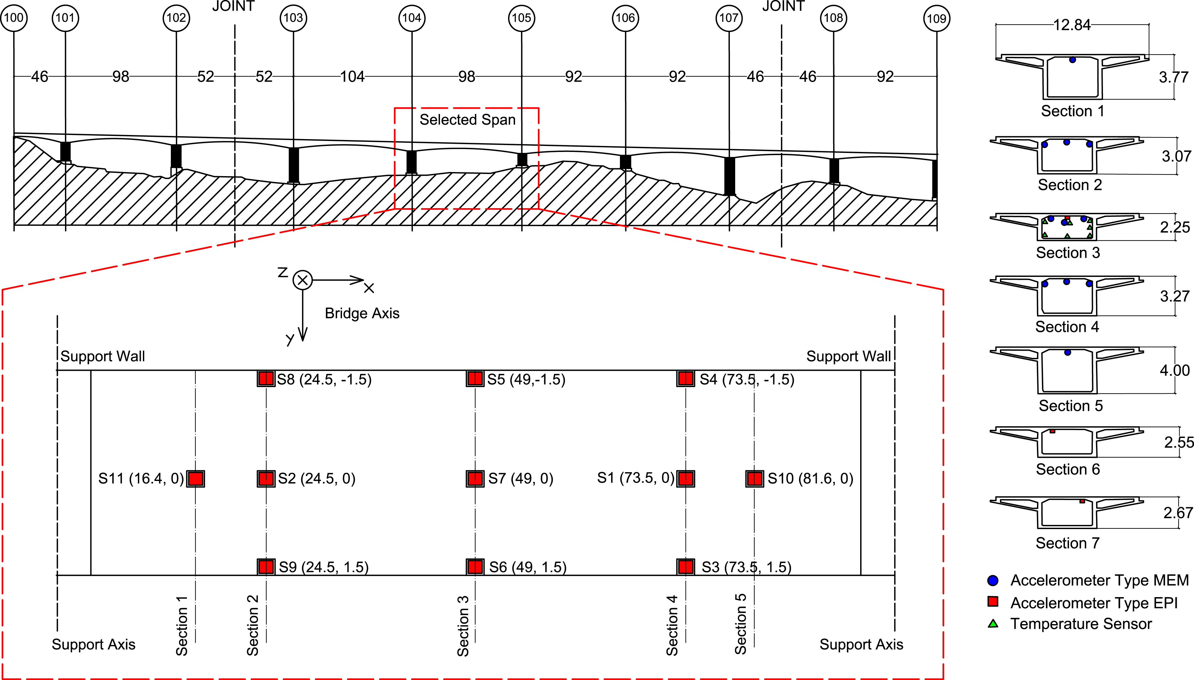

The available experimental data used in this study covers the period from March 24, 2017, to June 9, 2017, with a technical interruption between May 10 and May 29.

The raw acceleration signals undergo preprocessing, including filtering and detrending. A 100th-order FIR band-pass filter (0.5–24 Hz) is applied to eliminate irrelevant frequency components, given that the first natural frequency is 1.17 Hz. This SHM campaign provides essential information on the dynamic behavior of the viaduct and supports advanced monitoring strategies discussed in the thesis.

MEMS sensors provide three key advantages that underpin the effectiveness of the proposed framework. First, their low power consumption and compact size enable continuous, long-term monitoring with minimal installation impact. MEMS accelerometers typically operate at micro-to milli-watt power levels and have millimeter-scale dimensions, allowing for permanent and non-intrusive deployment on large-scale infrastructures. ⁶⁶ This capability is essential for acquiring the long-term datasets required for training Gaussian Process Regression models and supporting climate-based analyses. Second, MEMS accelerometers offer adequate sensitivity and dynamic range for civil engineering applications. Modern devices achieve sub-mg resolution and operate over frequency ranges spanning approximately 0.1 Hz to 1 kHz, ⁶⁷ which are well aligned with the low-frequency dynamics of large structures. In the case study considered herein, the first natural frequency of the bridge is approximately 1.17 Hz, while vibration data are acquired at 100 Hz, ensuring sufficient resolution for reliable automated operational modal analysis. Third, MEMS technology enables scalable and cost-effective monitoring solutions. Compared to traditional sensing systems, MEMS devices are relatively inexpensive and can therefore be deployed in dense configurations. This allows for improved spatial resolution of the structural response, which is particularly beneficial for multivariate analyses such as cointegration, as well as for enhancing damage detectability and localization capabilities. These characteristics are consistent with recent advances in MEMS-based sensing technologies for structural monitoring.^66,67

3.2. System identification

For each 10-minute sampling interval, modes are extracted using the SSI method, applying Hard and Soft Validation Criteria to ensure reliability as described in Section 2.1. After applying HVC and SVC, each measurement point was assigned to a corresponding mode. However, to enhance the reliability of the modal identification, an additional data cleaning step to perform outlier removal was performed using the Mahalanobis distance. ⁶⁸ This method identifies outliers as points that deviate significantly along the directions of greatest variability, effectively capturing anomalies that may be masked when using other distance metrics, such as the Euclidean distance. This approach is particularly effective in multivariate datasets, where correlations between variables can cause traditional distance-based metrics to misclassify points. Consequently, the Mahalanobis distance provides a more robust, statistically grounded criterion for detecting points inconsistent with the expected mode pattern.

Although a large number of modes were identified, only the eight bending-dominated modes consistent with the reference results of Martin-Sanz et al. ⁶⁹ were retained to ensure a meaningful comparison and minimize discrepancies due to environmental or computational factors. Table 1 summarizes the comparison between the two studies. Overall, the identified frequencies show excellent agreement with those reported by Martin-Sanz et al., ⁶⁹ confirming the consistency and reliability of the automated identification procedure. Minor discrepancies, within a few percent, can be attributed to differences in environmental conditions, sensor configurations, and processing settings. Notably, Mode 32 reported by Martin-Sanz et al., ⁶⁹ with a frequency of 16.694 Hz, was excluded, as it likely corresponds to an electromagnetic interference frequency (16.7 Hz) rather than a true structural mode.

Table 1.

Comparison with identified features by Martin-Sanz et al. ⁶⁹ (dataset April 4, 5:50 a.m.).

Mode	Martin-Sanz et al. 69		This work
	Frequency [Hz]	Damping [-]	Frequency [Hz]	Damping [-]
1	1.17	0.012	1.17	0.009
3	1.55	0.015	1.54	0.012
5	1.90	0.011	1.95	0.024
13	3.70	0.006	3.66	0.006
21	5.63	0.021	5.50	0.009
23	6.73	0.009	6.74	0.017
28	7.82	0.003	7.72	0.012
31	13.95	0.014	13.81	0.010
32	16.69	0.001	16.69	0.001

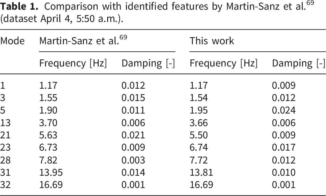
A higher discrepancy is observed in the damping ratios reported in Table 1 compared with the corresponding natural frequencies. This is expected from the extensive literature, since damping estimates obtained from output-only ambient-vibration data are generally more sensitive to signal quality, record length, environmental and operational variability, and the specific identification settings and estimator adopted.^42,70

Figure 4 presents the relationship between the identified natural frequencies of the Chillon Viaduct and the corresponding temperature measurements. The gray points represent the raw results obtained prior to filtering, while the colored points correspond to the modes retained after applying the Hard and Soft Validation Criteria. The filtering process effectively removes spurious estimates and clarifies the underlying linear dependence between frequency and temperature, thereby improving the consistency and reliability of the modal identification.

Figure 4.

Chillon viaduct frequencies in function of temperature. Grey points represent unfiltered results. Colored points are the results after the outlier removal step.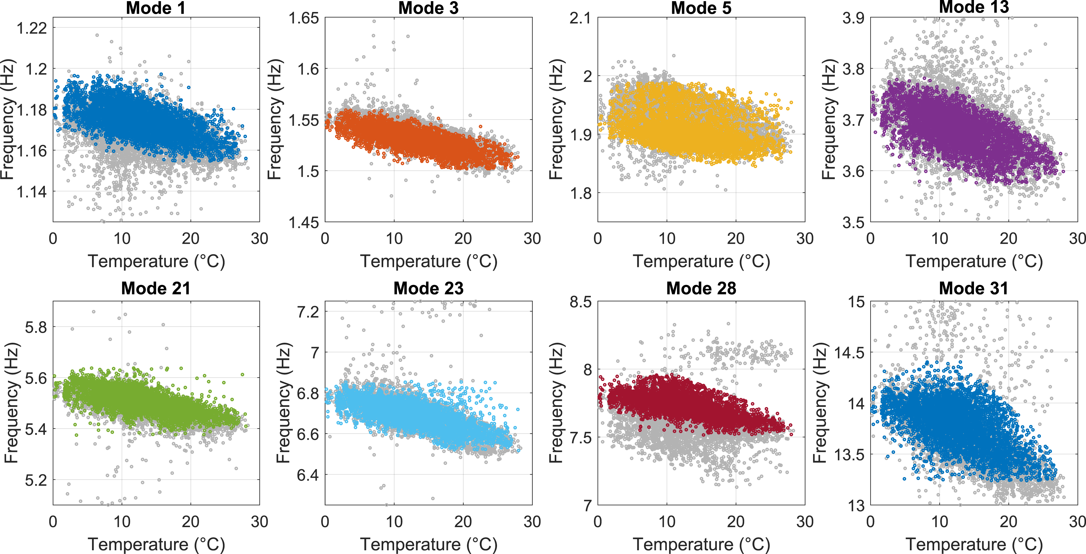

The natural frequencies of the Chillon Viaduct exhibit distinct temporal fluctuations throughout the monitoring period, displaying both diurnal and seasonal variability that closely follow changes in ambient temperature (Figure 5). This behavior reflects the strong temperature dependence of the bridge’s dynamic properties, evident also in Figure 4: as temperature increases, natural frequencies exhibit a consistent reduction. While this trend is often linked to temperature-dependent material softening, it reflects the combined effect of several thermally driven mechanisms, including changes in constitutive material properties, boundary-condition behavior, and potential stress-state changes induced by restrained thermal deformation. Given that this study follows a data-driven monitoring approach rather than a thermo-mechanical finite-element decomposition, we do not attempt to separately quantify each mechanism; however, the temperature-induced lowering of natural frequencies is a well-documented phenomenon proven in numerous legacy and recent field tests.

Figure 5.

Results of frequencies identified for the Chillon Viaduct leveraging the AOMA SSI colored by the temperature.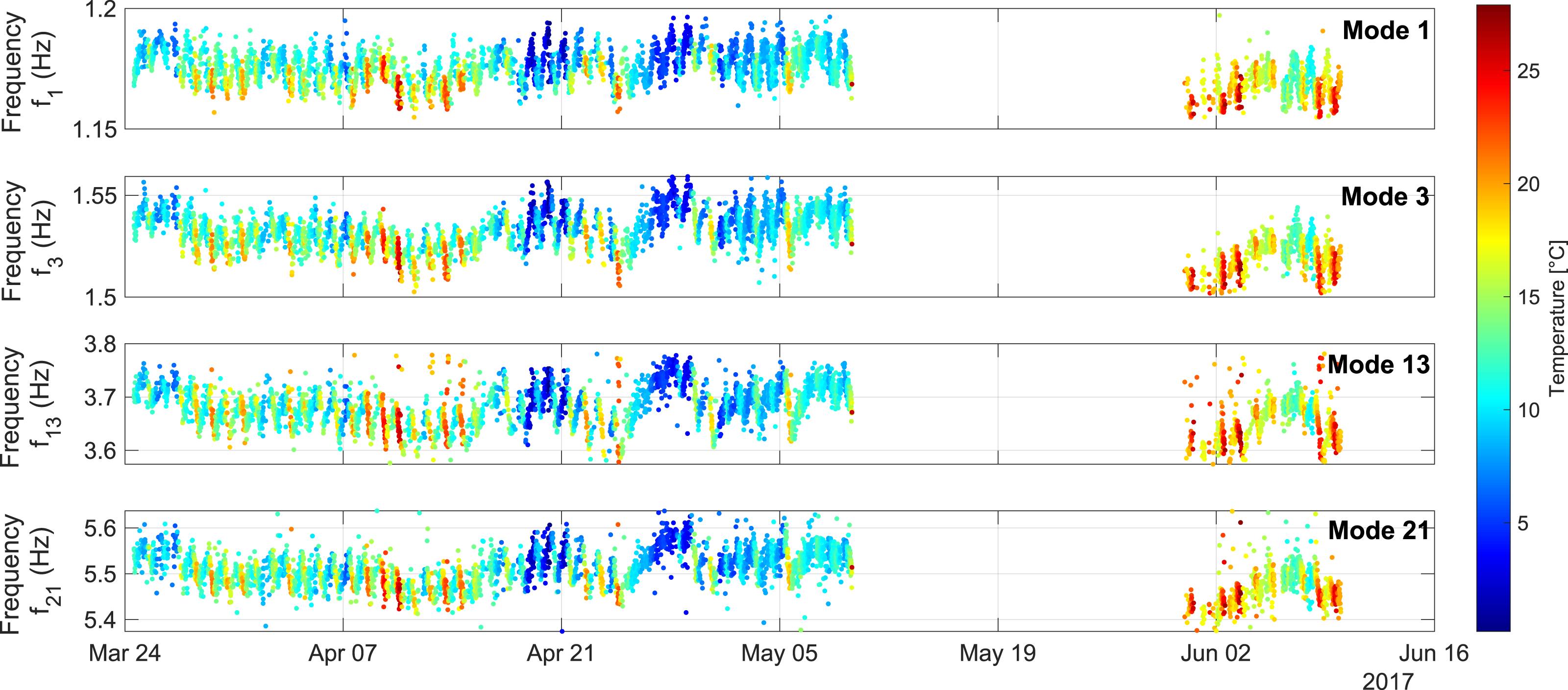

Moreover, a noticeable thermal lag is observed between the external and internal temperature measurements, attributable to the high thermal inertia of the concrete deck. This lag indicates that internal structural components respond to ambient temperature variations with a delay, a phenomenon that should be carefully considered when interpreting frequency–temperature relationships in long-term monitoring data.

The identified mode shapes (Figure 6) predominantly exhibit vertical bending behavior, consistent with the use of vertical accelerometer measurements. It is worth noting that, as reported by Martin-Sanz et al. ⁶⁹ due to the continuity of the deck, the structure cannot be interpreted as an isolated single-span beam, but rather as a portion of a continuous multi-span system. Consequently, different global modes of the viaduct may exhibit locally similar deformation patterns within the instrumented span, especially near the supports where small variations in deformation reflect different modal behavior. For this reason, the first three identified modes appear to correspond to a first vertical bending mode, with slight variations associated with the continuous configuration of the deck. Higher modes capture successive orders of vertical bending: Modes 13 and 21 correspond to the second-order response, Modes 23 and 28 to the fourth-order, and Mode 31 to the third-order mode. In contrast to natural frequencies, which are sensitive to environmental conditions, mode shapes remain largely invariant over time unless boundary conditions, such as support stiffness or expansion joint behavior, undergo significant changes. This stability makes them a valuable reference for detecting structural alterations and validating the consistency of the identified dynamic behavior.

Figure 6.

Identified mode shapes corresponding to the modes presented by Martin-Sanz et al., ⁶⁹ on April 4, at 5:50 a.m.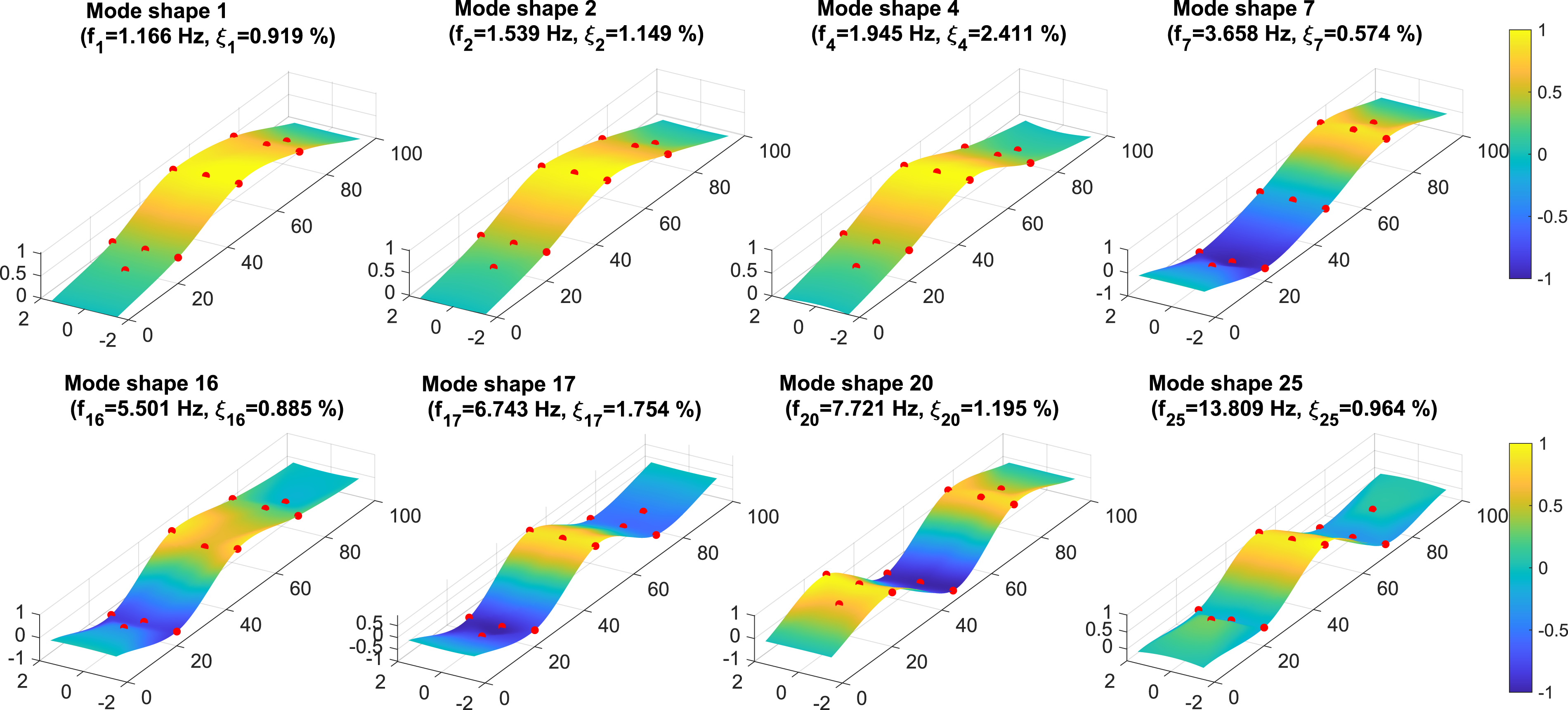

3.3 Climate change and scenarios

To project the evolution of temperature through the year 2100, this study employed the CH2018 regional climate model, ⁴³ which was specifically developed to assess future climate changes in Switzerland, with an emphasis on local temperature variability. This regionalization is essential for evaluating the potential long-term effects of climate change on the Chillon Viaduct. The CH2018 framework and its underlying dataset are comprehensively documented in the CH2018 Technical Report. ⁷¹

The CH2018 projections are derived from multiple Representative Concentration Pathway (RCP) scenarios,^44,72 reflecting different trajectories of greenhouse gas emissions and mitigation efforts:

• RCP 2.6: A low-emission scenario assuming strong mitigation actions that limit global warming to approximately 2°C above pre-industrial levels by 2100.

• RCP 4.5: An intermediate scenario with emissions peaking mid-century and gradually declining, resulting in a projected global temperature rise of 2–3°C by 2100.

• RCP 8.5: A high-emissions scenario without mitigation, representing a continued fossil fuel–intensive trajectory. This pathway anticipates a global temperature increase exceeding 4 °C by 2100 and is typically regarded as the most severe case for impact assessments.

The CH2018 dataset ⁴³ includes daily temperature series for the period 1981–2099, available for individual Swiss meteorological stations. For this study, data from the Aigle station (46.3181° N, 6.9706° E) were used, as it is the closest to the Chillon Viaduct, approximately 10 km away, a distance considered negligible for the analysis.

CH2018 integrates dynamic and statistical downscaling methods, including quantile mapping, to refine local projections using boundary conditions from the EURO-CORDEX ensemble of global climate models. Quantile mapping serves as a bias-correction technique that aligns the statistical distribution of simulated data with observed records, thereby improving the fidelity of temperature projections at the local scale. The results are depicted in Figure 7.

Figure 7.

Temperature predictions until 2100 according to different RCPs resulting from ”one vote per model” ensemble with CH2018 climatic models.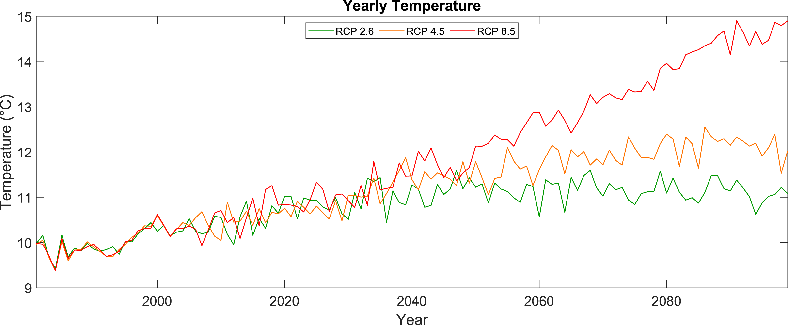

To account for the uncertainties inherent in the climate models, a “one vote per model” ensemble approach was adopted. ⁴⁴ This method combines predictions from multiple climate models within the CH2018 framework, assigning equal weight to each model to calculate the ensemble mean and standard deviation for each RCP scenario (Figure 8). This provides a central trend in future temperature projections and quantifies the variability among different models. More technical details can be found in the technical report ”Climate Change 2013: The Physical Science Basis” ⁴⁴ and in the publication ”Climate Scenarios for Switzerland CH2018 – Approach and Implications”. ⁷³

Figure 8.

Daily temperature projections under the RCP 2.6, 4.5, and 8.5 scenarios up to 2100 compared with daily values of temperature monitored on Chillon Viaduct.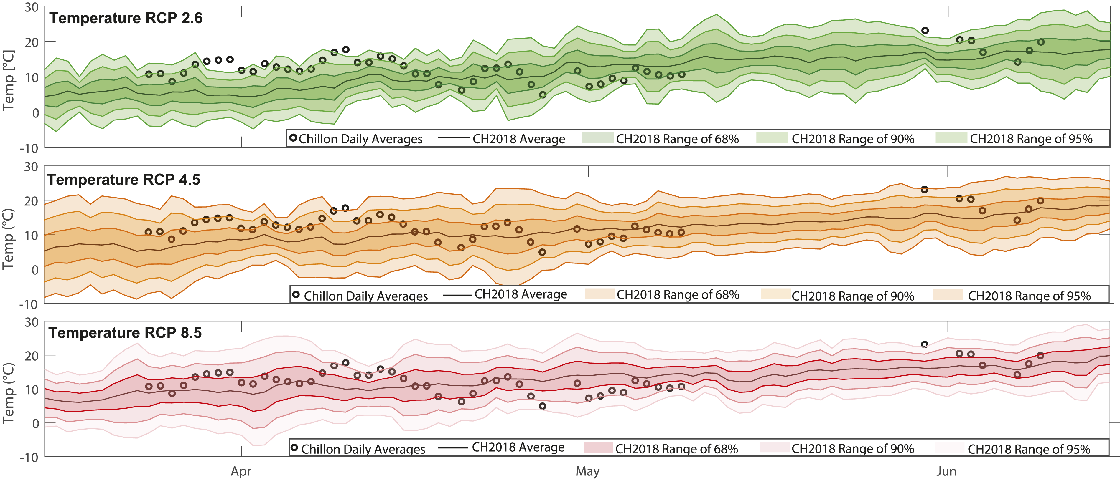

As a result, the CH2018 model provides daily near-surface temperature forecasts at the Aigle station through 2100 under different RCP scenarios. These projections were then used as input for the GPR model to predict the evolution of the natural frequencies of the Chillon Viaduct in response to future climate change.

3.4. Gaussian process on the Chillon Viaduct

The target natural frequencies were modeled using a GPR framework designed to capture both long-term thermal effects and short-term cyclic variability. The model was formulated with temperature and time as input variables, enabling the joint representation of environmental and temporal dependencies within a unified probabilistic structure. The covariance structure employs an additive kernel composed of a linear component, which models the approximately linear sensitivity of frequency to thermal variations, and a periodic component designed to capture the diurnal cycles inherent in the structural dynamic response. This integrated linear-periodic kernel is defined as:

$k\left((t,T),(t^{\prime },T^{\prime })\right)={\sigma }_{\text{lin}}^{2}T{T}^{\prime }+{\sigma }_p^2\exp \left[-\frac{2}{{\ell }_p^2}{\sin }^2\left(\frac{\pi }{P}(t-t^{\prime })\right)\right],$

(5)

where t denotes the absolute time in days, T is the standardized temperature, P = 1 day is the fixed daily period, and σ_lin, σ _p , ℓ _p are kernel hyperparameters controlling, respectively, the scale of the linear temperature contribution, the variance of the periodic component, and its characteristic smoothness.

This kernel structure allows the GP to capture both long-term thermal correlations (via the linear term k _lin ) and recurrent daily fluctuations (via the periodic term k _per ). The hyperparameters are initialized to physically meaningful values: σ_lin ≈ 0.1 (frequency sensitivity to temperature), σ _p ≈ 0.05, and ℓ _p ≈ 0.5 days (daily smoothness). Optimization is performed by maximizing the marginal logarithmic likelihood. The observation-noise variance was treated as a GP hyperparameter and estimated by maximizing the marginal log-likelihood. The resulting noise contribution was then incorporated into the predictive uncertainty.

Given the high density and extensive temporal span of the Chillon Viaduct dataset, a sparse GPR approximation was implemented to maintain computational tractability without compromising predictive uncertainty. This approach utilizes a subset of 100–250 inducing points, representing approximately 15% of the thinned training data, to summarize the global information content while preserving the integrity of the probabilistic bounds. While relative humidity was initially considered as a secondary covariate, it was eventually omitted from the final architecture due to its marginal contribution to predictive accuracy and the absence of reliable long-term climate projections for this variable.

The baseline established by this kernel structure successfully captures the environmental variability of the natural frequencies, thereby providing a stabilized signal for the isolation of potential structural anomalies. Model validation was conducted by partitioning the data from January to May into alternating training and testing windows with a 70/30 split, with June reserved as an independent hold-out set for final evaluation.

Several covariance kernels were tested for the residual component of the GPR, including Squared Exponential (SE), Matérn 3/2, Periodic, Quasi-Periodic (SE× Periodic), and Linear (time and/or temperature). Each kernel was optimized via log-marginal-likelihood maximization and validated on unseen data. The analytical expressions and performance metrics of all the tested kernels are summarized in Table 2. Some formulations, such as the Matérn or complex quasi-periodic combinations, showed overfitting, very low training errors but poor generalization, whereas simpler formulations, such as the single SE kernel, yielded excessive prediction errors. As a balanced solution between flexibility and robustness, the additive combination of a linear and a periodic kernel (k = k_lin(T) + k_per(t)) was selected, effectively capturing the approximately linear temperature dependence of the natural frequencies together with recurrent diurnal fluctuations, while maintaining consistent predictive accuracy.

Table 2.

Comparison of GPR kernel formulations and corresponding training and testing RMSE values. The variables t, t′ represent time inputs; T, T′ temperature inputs; x, x′ generic input feature vector; r = |x − x′| the Euclidean distance. σ² denotes process variance, ${\sigma }_t^2$ and ${\sigma }_T^2$ are linear scaling coefficients, l, l _t , l _p are characteristic length scales, and p is the period of the periodic kernel. Subscripts k_lin, k_SE, and k_per denote linear, squared exponential, and periodic components, respectively. In bold the final choice of the kernel for the study.

Name	Kernel formula	RMSEtrain [Hz]	RMSEtest [Hz]
Quasi-Periodic	$k={\sigma }^2\exp \left(-{(t-t^{\prime })}^2/2l_t^2\right)\exp \left(-2{\sin }^2(\pi |t-t^{\prime }|/p)/l_p^2\right)$	0.0010	0.0068
Squared Exponential	$k={\sigma }^2\exp \left(-{(x-x^{\prime })}^2/2l^2\right)$	0.038	0.0096
Matérn 3/2	$k={\sigma }^2\left(1+\sqrt{3}r/l\right)\exp \left(-\sqrt{3}r/l\right)$	0.0009	0.1185
Periodic	$k={\sigma }^2\exp \left(-2{\sin }^2(\pi |t-t^{\prime }|/p)/l^2\right)$	0.0046	0.0060
Linear (Time + Temperature)	$k={\sigma }_t^{2}t{t}^{\prime }+{\sigma }_T^{2}T{T}^{\prime }$	0.0046	0.0061
Additive Linear (t + T)	k = klin(t) + klin(T)	0.0047	0.0054
Multiplicative Linear–Periodic	k = klin(T) × kper(t)	0.0046	0.0052
Additive Linear–Periodic	k = k lin (T) + k per (t)	0.0045	0.0052
Additive SE–Periodic	k = kSE + kper	0.0008	0.0049
Multiplicative SE–Periodic	k = kSE × kper	0.0009	0.0052

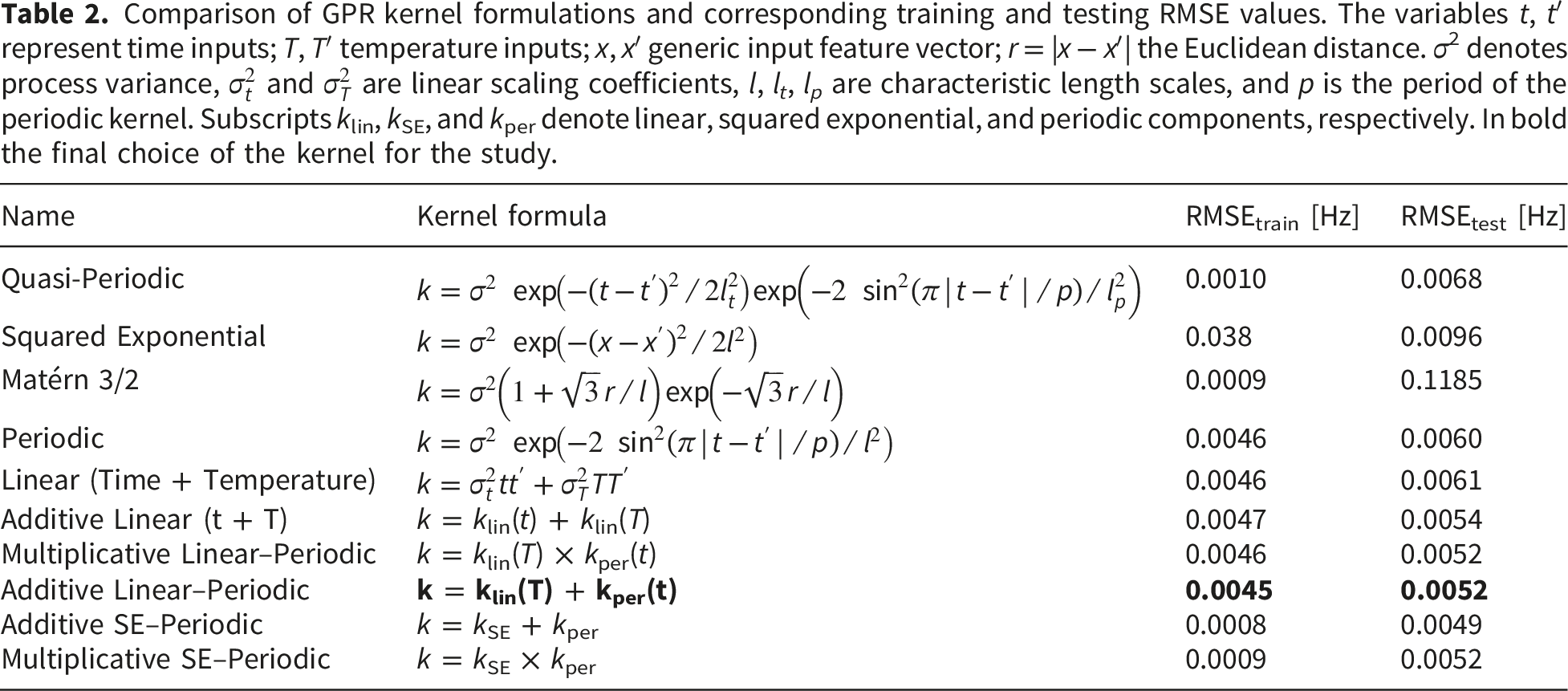
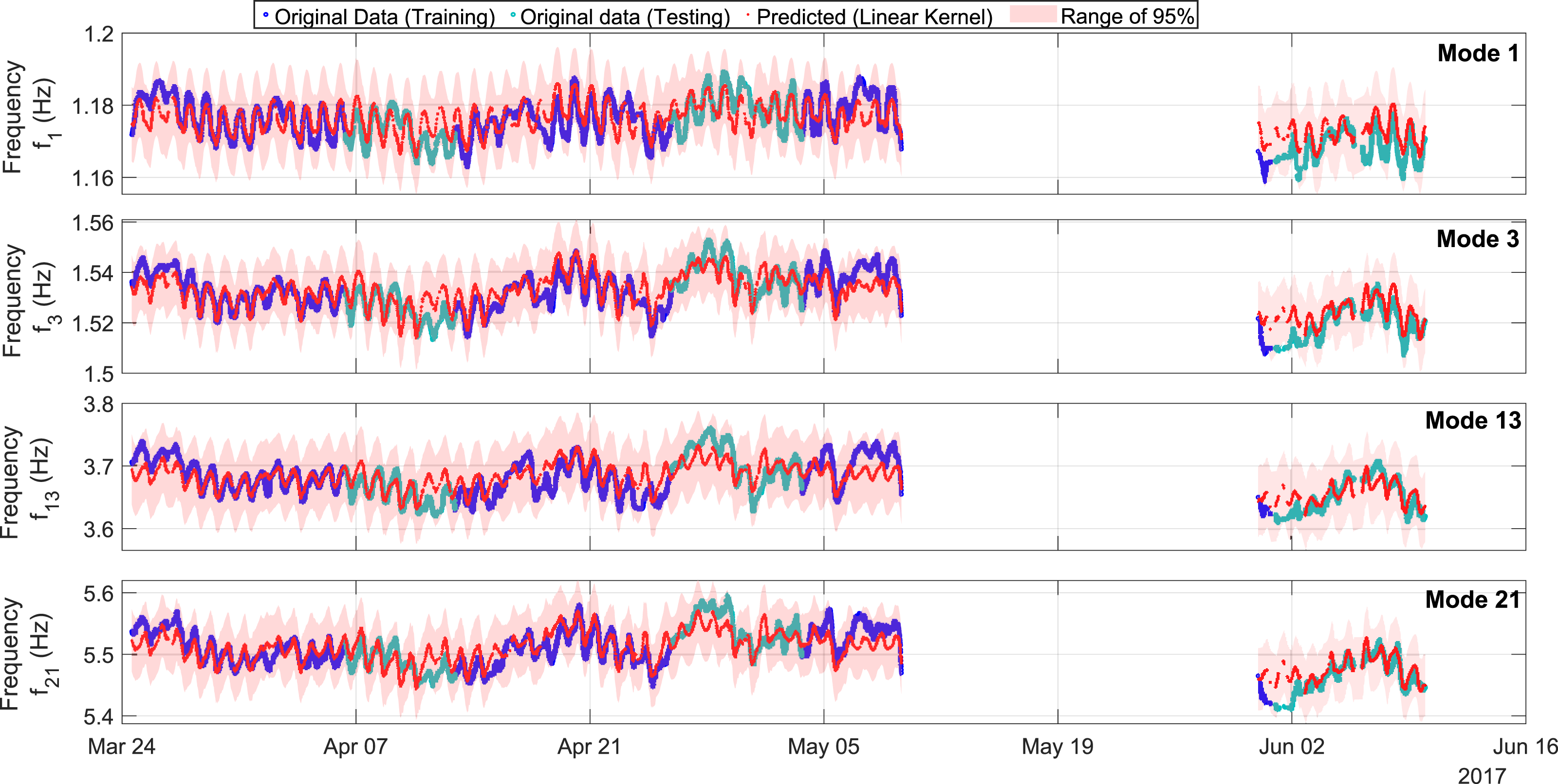
The time series of identified natural frequencies was preprocessed using moving averages of varying window lengths (1 hour and 3 hours) to attenuate high-frequency components and minimize stochastic variance. In the context of AOMA, these fluctuations are primarily attributed to identification uncertainty, which is a manifestation of the statistical variability inherent in the Stochastic Subspace Identification algorithm and the random nature of ambient excitation sources. To mitigate this noise, an 18-point moving average was adopted for the GPR modeling, corresponding to a 3-hour interval at the 10-minute sampling rate. This window size represents an optimal compromise between noise suppression and temporal resolution, as it effectively filters the identification noise while preserving the thermo-dependent response of the structure. This filtering step is essential to emphasize meaningful structural trends, prevent the GPR model from overfitting to estimation errors, and ensure that predictive trends represent physically significant structural variations rather than algorithmic instabilities. Figure 9 illustrates the impact of these smoothing regimes on the f₃ time series, where the narrowing of the statistical distributions highlights the reduction in identification-driven dispersion. Subsequently, Figure 10 presents the natural frequencies predicted over time for the best temperature-related vibration modes, along with the uncertainty interval.

Figure 9.

Time series of f₃ with different moving means compared with the original signal without a moving mean.

Figure 10.

Predicted natural frequencies over time with the uncertainty range represented by the 1.96 times standard deviation.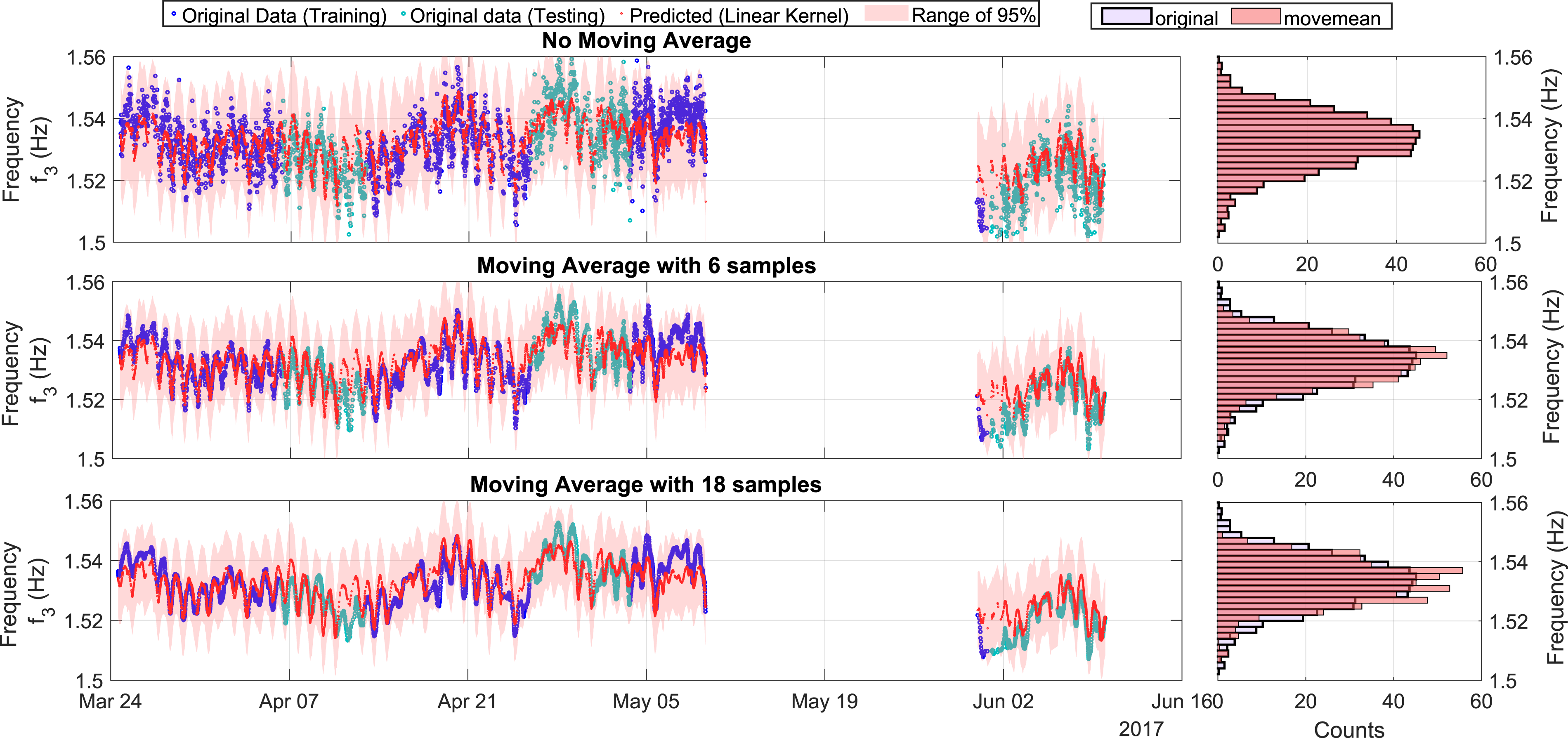

The performance of the GPR model was assessed using several quantitative metrics for both training and test sets. These metrics include Mean Absolute Error (MAE), Root Mean Square Error (RMSE), Relative Root Mean Square Error (rRMSE), and the Time Response Assurance Criterion (TRAC). Figure 11 displays the values of these metrics for the eight analyzed modes, providing a comprehensive evaluation of the model’s predictive accuracy relative to the observed data. The analysis shows that the absolute error increases slightly with the mode’s natural frequency, reaching a maximum at the highest one. Despite this, the overall accuracy remains high, and the difference between MAE and RMSE indicates only a few larger deviations that do not affect the model’s reliability. When the error is expressed in relative terms, differences among modes become negligible, confirming a uniform predictive accuracy across all frequencies. The TRAC metric remains close to 1 across all modes, though it is less informative in this context because it cannot effectively capture larger discrepancies. Finally, the close agreement between training and testing errors demonstrates that the Gaussian Process Regression model generalizes well, successfully capturing the relationship between temperature and natural frequencies without overfitting.

Figure 11.

Evaluation of the GPR model’s prediction performance using various metrics.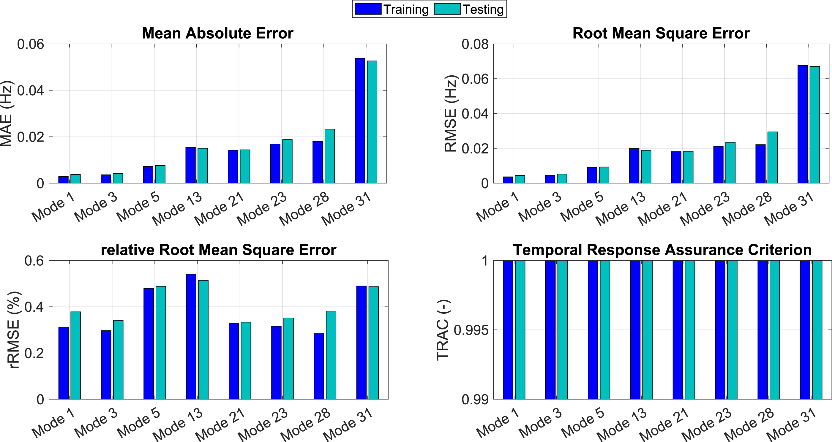

Figure 12 compares the predicted natural frequencies with the measured frequencies in the entire dataset. The concentration of data points along the 45-degree bisector serves as a primary indicator of strong mutual correlation, demonstrating that the model effectively captures the underlying structural dynamics under varying environmental conditions. A critical aspect of these results is the performance of the probabilistic confidence bounds, represented by the shaded regions, which illustrate the model’s quantified uncertainty at a 95% confidence level. The containment of the majority of identified frequencies within these intervals validates the reliability of the GPR framework in providing a calibrated measure of prediction error alongside the mean estimates. While the general alignment confirms high predictive fidelity, the localized dispersions observed in certain modes suggest residual estimation errors or minor unmodeled physical phenomena, such as non-linear thermal lags, which the model accounts for through its expanded uncertainty bounds.

Figure 12.

Comparison between predicted and measured frequencies in the training and test sets.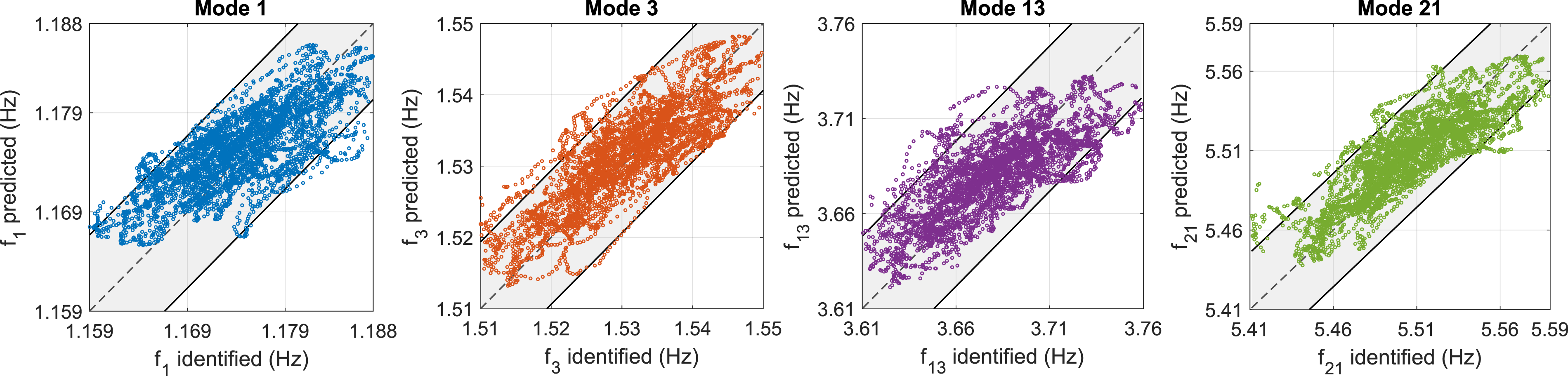

The GPR residuals represent the difference between predicted and measured natural frequencies, providing a fundamental metric for evaluating potential prediction errors. By incorporating temperature as an input variable, the GPR model effectively learns to eliminate the deterministic influence of thermal variations on the structural response. Consequently, under normal operating conditions, these residuals are expected to exhibit stationary behavior, as they are essentially stripped of systematic temperature-induced trends.

This stationarity is a critical property that renders GPR residuals highly suitable as inputs for cointegration analysis. By utilizing these residuals, the framework provides a robust, alternative method for isolating subtle structural damage signals from dominant environmental effects. For a structure in an undamaged state, these cointegrated residuals should remain stable and stationary. Figure 13 reports the residuals obtained in the present case study, showing their stationary behavior once the temperature influence has been removed.

Figure 13.

Residuals between the predicted and measured frequencies.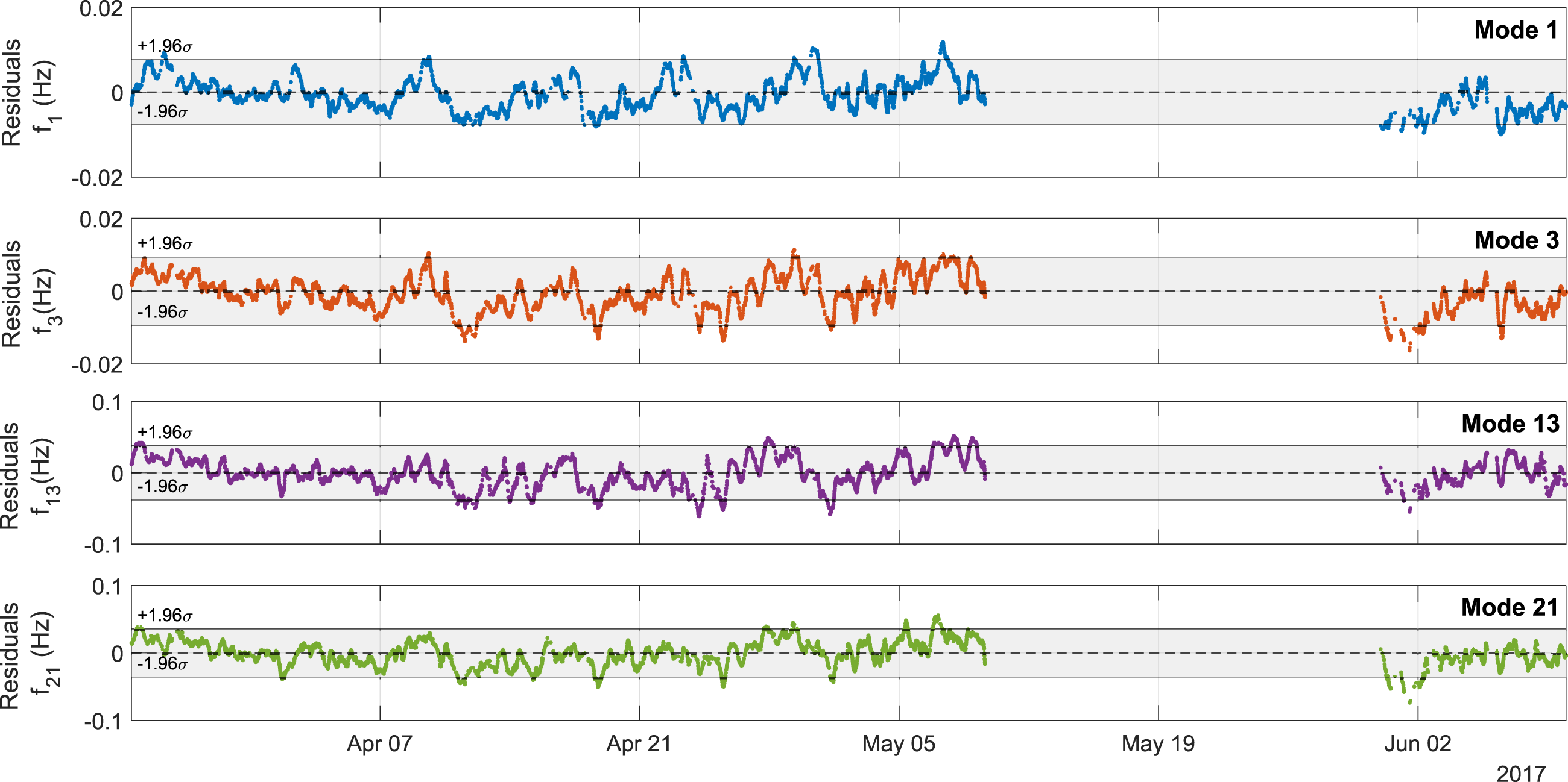

3.5 Results of cointegration analysis

The performance of the proposed anomaly detection framework was evaluated by analyzing the statistical properties of the GPR residuals: the healthy baseline, simulated progressive damage, and long-term operational scenarios involving climate drift versus fatigue. Moreover, a distinction was made between the empirical dispersion of the observed residuals and the predictive uncertainty propagated from the Gaussian Process model.

3.5.1 Baseline validation and environmental compensation

The residuals are defined as the difference between the measured natural frequencies f _meas (t) and the GPR mean prediction μ _GP (t). Two distinct measures of uncertainty were analyzed to ensure a scientifically sound detection threshold: 1) the GP predictive uncertainty (σ _GP ) that represents the probabilistic confidence of the model, derived from the posterior covariance matrix of the Gaussian Process. It accounts for both the observation noise learned during training and the lack of data in certain thermal regimes. The 95% confidence interval of the model is defined as ± 1.96σ _GP ; 2) the empirical residual deviation (σ _res ) that indicates the standard deviation computed from the actual residual time series during the healthy baseline period. It captures the total realized variance of the system, including measurement noise and any minor environmental effects not fully compensated by the kernel.

For Statistical Process Control (SPC), operational thresholds were established based on the empirical standard deviation σ _res . The Upper and Lower Control Limits (UCL, LCL) were set at ± 3σ _res (corresponding to a 99.7% confidence level under the assumption of normality). This approach ensures that the detection thresholds reflect the actual variability of the structure rather than the theoretical confidence of the model.

The residuals derived from the GPR predictions for the historical dataset (undamaged state) are presented in Figure 14. Visual inspection confirms that the time series is centered around zero and exhibits stable variance over the monitoring period. The residual signal remains predominantly within the UCL and LCL defined by the ± 3σ threshold, with only negligible transient excursions observed in the test set that do not indicate systematic drift. Comparing the two uncertainty measures reveals that the empirical deviation σ _res is consistent with the GP predictive uncertainty. This alignment indicates that the GPR model is well-calibrated: the actual scatter of the residuals falls within the range predicted by the model’s probabilistic bounds.

Figure 14.

Residuals of f₃ with GP.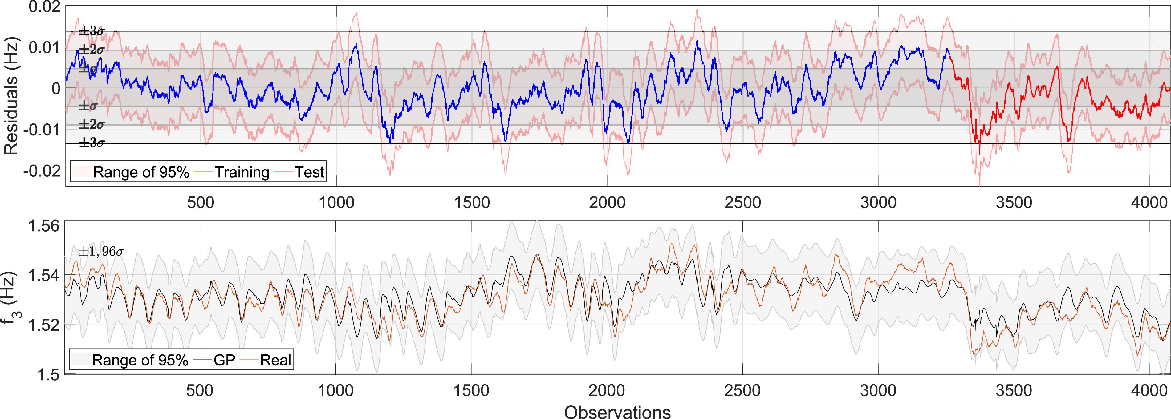

To rigorously verify the removal of environmental trends, the ADF test was performed on the residual sequence. The test rejected the null hypothesis of a unit root at the 1% significance level, confirming stationarity (I(0)). This result empirically validates that the GPR model has effectively captured the non-linear thermal dependencies, yielding a feature set that is robust to normal environmental variability and free of systematic drifts.

The sensitivity of the framework was evaluated by simulating a progressive loss of stiffness, modeled as a linear reduction in natural frequencies from 0% to 3% over the final phase of the monitoring period.

Figure 15 illustrates the evolution of the residuals under this scenario. The plot explicitly compares the empirical control limits ( ± 3σ _res , indicated by black horizontal lines) against the GP predictive uncertainty (the 95% confidence interval, shown as the grey shaded region). 9 During the healthy phase (indices 0–3300), the residuals oscillate around zero and remain strictly bounded by the ± 3σ _res limits, validating the null hypothesis of structural integrity. However, upon the initiation of damage (approx. index 3300), a distinct deterministic trend emerges. The residuals exhibit a monotonic deviation toward negative values, rapidly breaching the LCL.

Figure 15.

Residuals of f₃ with GP with incremental damage of 0-3%.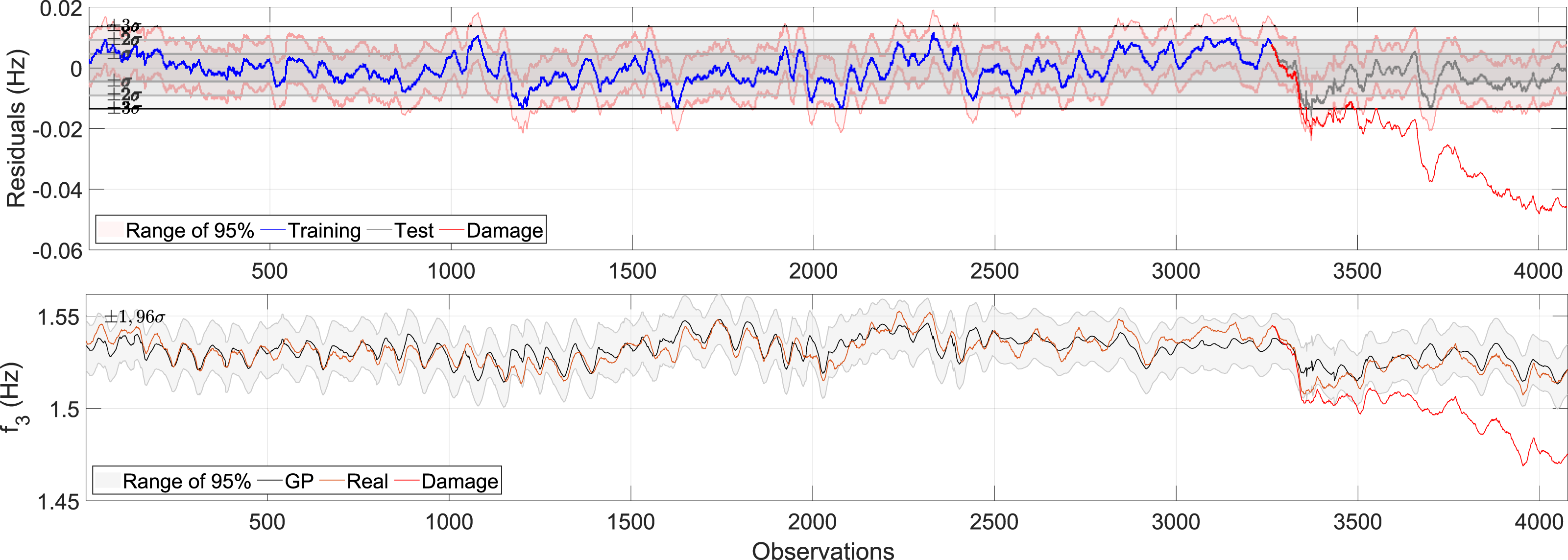

Crucially, the GP predictive uncertainty (the grey band) does not expand during this period. This stability indicates that the model remains confident in its prediction of the ”healthy” thermal baseline. Consequently, the excursion of the red residual line outside the grey confidence band confirms that the deviation is not attributable to epistemic uncertainty (e.g., extrapolation to unknown temperatures) but rather to a physical change in the system’s stiffness that contradicts the learned thermal model. This divergence effectively triggers the detection of the anomaly well before the damage magnitude reaches its 3% maximum.

3.5.2 Operational resilience: Climate vs. fatigue scenarios

To verify the system’s operational resilience, the framework was stress-tested against two distinct long-term scenarios: gradual climate drift versus rapid fatigue accumulation. This comparison is critical for distinguishing between environmental trends and structural degradation.

This comparison is critical for ensuring that maintenance resources are prioritized for genuine structural risks rather than environmental noise. The operational response to the CH2018 climate projection is presented in Figure 16. In this scenario, a temperature-induced frequency reduction of approximately 0.13% was simulated over a decade. The upper panels, which display the time history of the cointegration residuals over the first three years, reveal that the signal remains stationary and predominantly contained within the empirical control limits. The underlying frequency tracking in the lower panels confirms this robustness; the GP prediction (black line) effectively overlaps with the structural response (green line), demonstrating that the model absorbs the slow, low-magnitude thermal drift without triggering false positives.

Figure 16.

Cointegration residuals (upper panels) and frequency tracking (lower panels) under the CH2018 climate scenario, simulating a 0.13% frequency reduction over 10 years. The residuals remain stationary and within the empirical control limits, indicating robustness to slow thermal drift.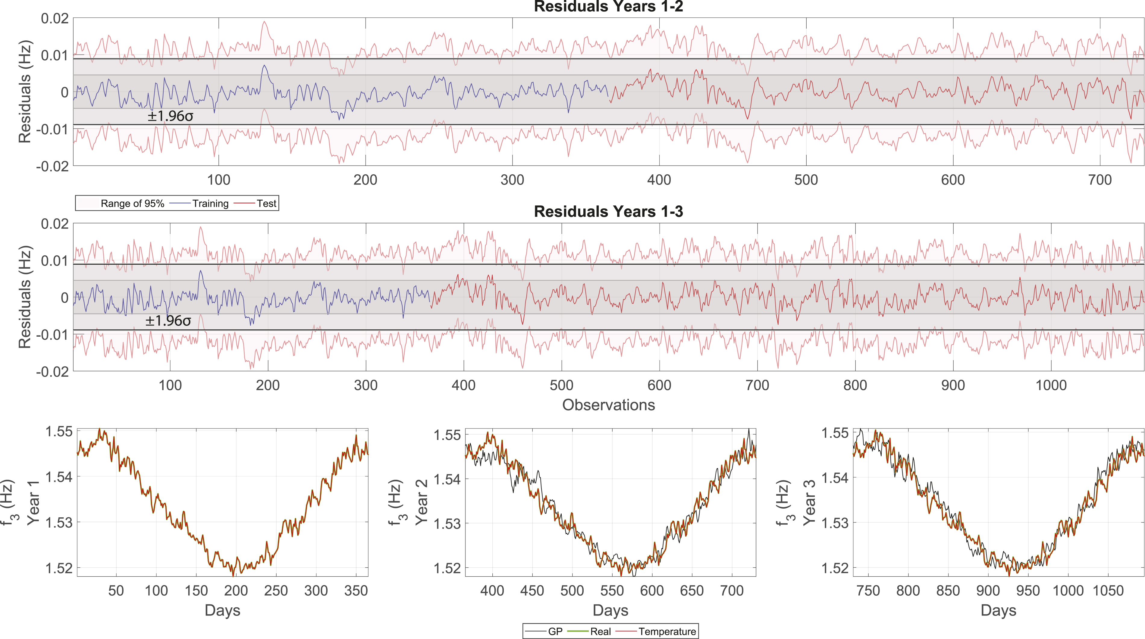

In sharp contrast, the system’s response to a fatigue scenario simulating a 2.5% annual frequency reduction is shown in Figure 17. Unlike the climate case, the residuals in the upper panels exhibit a clear deterministic, non-stationary trend that rapidly diverges from the zero mean. By the end of the third year, the residual signal has permanently breached the Lower Control Limit, signaling an anomaly. This divergence is physically evident in the frequency tracking panels, where the fatigue-induced response (red line) progressively separates from the healthy model prediction (black line). This dichotomy highlights the primary advantage of the proposed methodology: it effectively suppresses the manageable, long-term effects of climate change while maintaining high sensitivity to rapid deterioration mechanisms, ensuring that alarm thresholds remain meaningful and actionable.

Figure 17.

Cointegration residuals (upper panels) and frequency tracking (lower panels) under a simulated fatigue scenario with a 2.5% annual frequency reduction. The residuals exhibit a distinct non-stationary drift that breaches the control limits, confirming sensitivity to structural damage.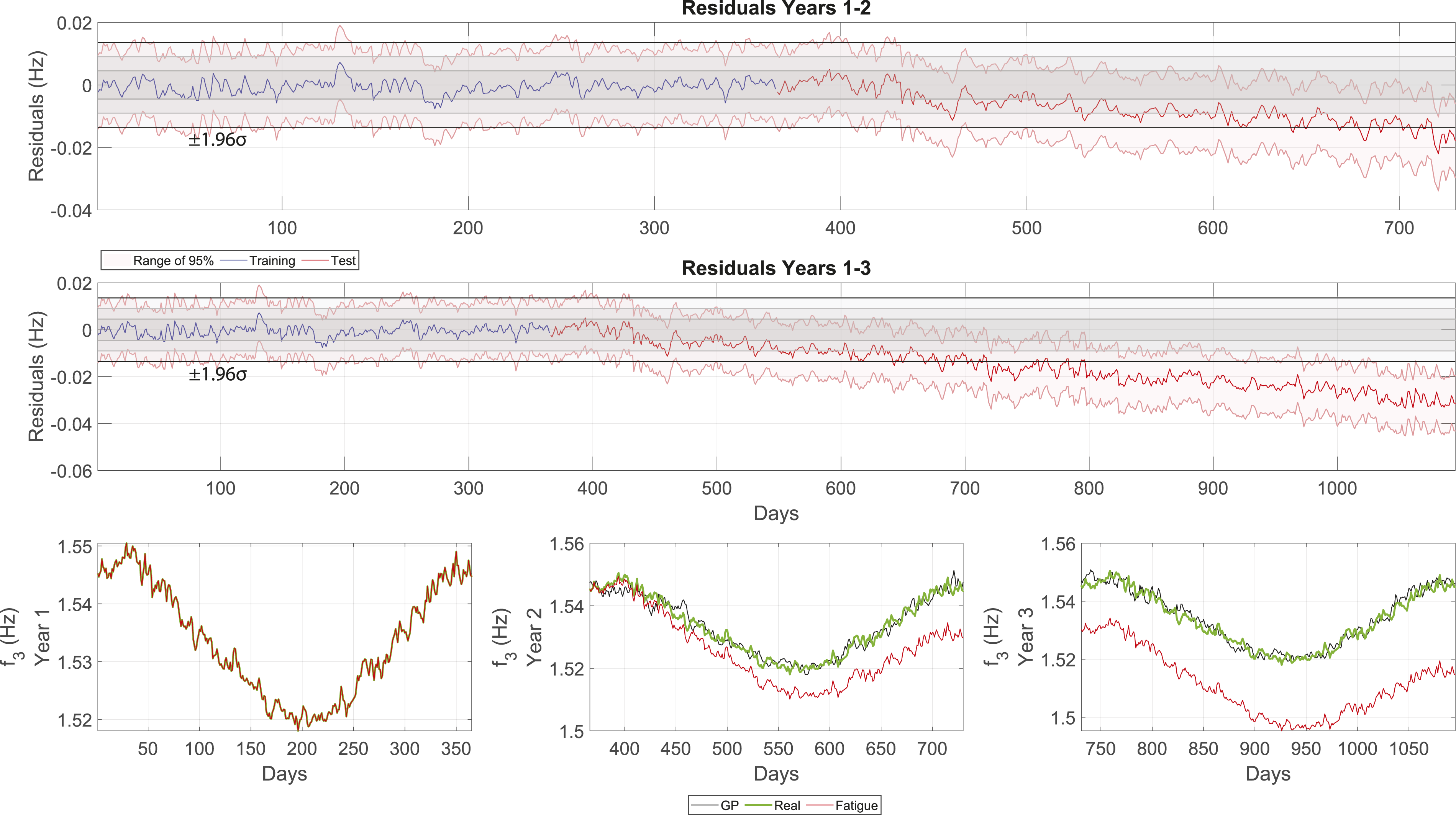

This comparison highlights a critical operational advantage: the methodology effectively filters out the negligible short-term effects of climate change while maintaining high sensitivity to rapid deterioration mechanisms. This selectivity ensures that maintenance resources are prioritized for genuine structural risks (e.g., fatigue) rather than for manageable environmental drifts.

4. Conclusion

This study presents a climate-resilient framework for Structural Health Monitoring to address the challenge of ensuring long-term infrastructure safety in the context of evolving environmental conditions. By integrating Automated Operational Modal Analysis, Sparse Gaussian Process Regression, and regional climate projections, the proposed methodology transforms the issue of environmental variability from a source of uncertainty into a manageable predictive parameter. The application of this framework to the Chillon Viaduct yielded primary insights regarding environmental dependency, long-term climate impact, and damage detection sensitivity.

The automated identification modal successfully characterized the dynamic behavior of the bridge, revealing a strong inverse correlation between temperature and natural frequencies, driven by the collective influence of material and structural thermal responses. The Sparse Gaussian Process Regression model effectively captured this dependency, providing a calibrated probabilistic baseline that accurately characterizes and models these thermal effects. By coupling the regression model with CH2018 climate projections, the study quantified the structural impact of global warming scenarios. Under the most severe Representative Concentration Pathway 8.5, the model projects a gradual frequency reduction of approximately 1% over the next century. Crucially, the analysis demonstrated that for shorter planning horizons of ten years, the climate-induced drift of approximately 0.13% is negligible compared to the natural variance of the identification process, allowing the system to maintain stationarity without triggering false alarms.

The cointegration analysis of regression residuals proved highly effective in decoupling environmental trends from structural anomalies. While the system absorbed the slow climate drift, it exhibited immediate sensitivity to simulated fatigue damage. A fatigue scenario with a 2.5% annual frequency reduction led the residuals to breach the lower control limit within the first year, thereby rejecting the stationarity hypothesis and clearly flagging structural risk. The primary contribution of this work is the validation of a robust baseline strategy that demonstrates that, when properly calibrated to climate scenarios, data-driven models can distinguish between benign, slow-onset drifts caused by climate change and malignant, rapid-onset shifts caused by structural degradation. This selectivity is operationally vital, ensuring that maintenance resources are prioritized for genuine structural risks rather than being wasted on false positives driven by uncompensated thermal trends.

Despite these advancements, the present framework has some limitations that define important directions for future research. First, the current methodology relies on a static training phase, implicitly assuming that the relationship between temperature and frequency remains invariant over decadal scales. This assumption may be challenged by material aging, progressive deterioration, or environmental conditions beyond the range represented in the training data. For this reason, future work will focus on developing online updating strategies that enable the regression model to continuously adapt to newly observed environmental regimes, thereby reducing epistemic uncertainty over time.

A second limitation of the present study is that the framework is demonstrated on a single case study only. Although the Chillon Viaduct provides a valuable real-world benchmark, additional validation on other structures, climates, and structural typologies will be necessary to assess the broader generalizability and transferability of the methodology. Moreover, the monitoring record used in this work does not span a full annual cycle and therefore does not include winter observations at the lowest temperatures. Nevertheless, the available dataset covers a substantial temperature range, approximately from 0 to 25°C, which is sufficient to identify the main temperature–frequency trend required by the proposed modeling framework. This range is also consistent with the average temperature regimes represented in the adopted climate projections. Longer monitoring records would nonetheless improve robustness under less frequently observed environmental conditions and further strengthen extrapolation under future climate scenarios.

More broadly, a natural extension of this research is the evolution of the proposed framework toward a more complete Digital Twin setting. In particular, future developments will consider coupling the current monitoring and anomaly-detection workflow with higher-fidelity structural representations, such as finite-element-based digital models, and enabling more explicit bidirectional updating between measured response and virtual system state. Another important direction concerns the integration of decision-support layers capable of translating uncertainty-aware monitoring outputs into maintenance-oriented actions. Future work will also explore the integration of the proposed probabilistic monitoring indicators with decision-support models. In particular, fuzzy multi-criteria decision frameworks, including hesitant and T-spherical fuzzy formulations, offer a promising pathway for translating GPR uncertainty bounds, cointegration residuals, climate-scenario variability, and sensor-confidence information into interpretable maintenance-oriented risk classes. Such an extension would complement the monitoring and inference layer developed in this study by supporting engineering decisions under combined aleatory and epistemic uncertainty. At the same time, the scalability of MEMS-based sensing networks supports the extension of the framework to other infrastructure systems where dense spatial measurements are required to capture complex structural dynamics.

Overall, this research bridges civil engineering, data science, and climate science by proposing a framework that not only compensates for environmental variability but also explicitly incorporates its future evolution into structural monitoring. In this sense, the methodology provides a scalable and climate-adaptive foundation for next-generation monitoring and, more broadly, for future infrastructure Digital Twin implementations.