Optimized design under uncertainties of a passive vibration control system for highway bridges considering the vehicle-bridge-pavement interaction

Abstract

Dynamic bridge analysis requires considering factors like material properties, vehicle velocity, mass, suspension, and road roughness, all of which are crucial for understanding the bridge’s behavior. Excessive vibrations can cause discomfort, reduce the structure’s service life, and even lead to collapse. Tuned Mass Dampers (TMDs) offer a reliable and economical solution to mitigate these vibrations. This work introduces a comprehensive methodology for optimizing TMDs, addressing the coupled vibration challenges across all involved systems (Bridge-Vehicle-Pavement-TMD) while incorporating uncertainties, making the design more robust against parameter variations. Three vehicle models are analyzed, including simulations of pavement roughness and obstacles at the bridge entrance. Uncertainties are accounted for using Monte Carlo simulation, enhancing the reliability of the results. The TMD parameters were designed using the HBA algorithm, and to further improve efficiency, the objective function was parallelized, resulting in a 60% reduction in computation time per iteration compared to a fully sequential code. This optimization under uncertainty led to a reduction in the mean maximum bridge displacement by over 7.5% on uneven pavement and 14.4% with obstacles. This robust optimization approach, combined with parallel processing, provides a useful tool to assist designers with the project of new structures or propose a solution to extend the service life of the existing ones.

1. Introduction

A bridge is a structure built to support the traffic of vehicles, people, or moving loads. It aims to overcome obstacles such as rivers, valleys, and intersections. ¹ Every day, various types of vehicles with different configurations, weights, and velocities travel on bridges. Thus, these structures are subjected to the dynamic effects provoked by the interaction with the vehicles and the pavement conditions.

To properly analyze the dynamic loading caused by traffic on a bridge, it is important to consider not only the bridge’s dynamic characteristics, such as its span and natural frequencies, but also various aspects of the vehicles using it, such as their suspension systems, weight, and velocity, as well as the pavement’s roughness profile.^2,3

Vibration, caused by the interaction of vehicles, structure, and pavement, poses a primary challenge for bridge integrity over its service life. A widely used solution is the Tuned Mass Damper (TMD), valued for its reliability, low maintenance, and energy-free operation. TMDs have demonstrated success in various applications, including the Rio-Niteroi Bridge, ⁴ Millennium Footbridge, ⁵ and FEUP footbridge. ⁶

With advancements in TMD design, several studies have demonstrated their effectiveness in vibration control. For instance, ⁷ showed that a single TMD at the center of a three-span bridge reduced dynamic response from high-speed trains. ⁸ investigated passive and semi-active devices for vibration reduction on bridges with moving loads. ⁹ explored multiple Tuned Mass Friction Dampers for high-speed railways, and ⁶ proposed a semi-active TMD to enhance vibration control on Porto University’s footbridge.

Tuned Mass Dampers (TMDs) are a practical solution for reducing vibrations in bridges caused by vehicular traffic. Research has focused on optimizing TMD design parameters to enhance their effectiveness and capacity. Among these works, it should be highlighted that ¹⁰ introduced a robust methodology for designing multiple TMDs (MTMDs) using the Firefly meta-heuristic algorithm. ¹¹ focused on multiple TMD designs with the Variable Accelerated Pattern Search algorithm (VAPS) to mitigate vehicle-induced vibrations on continuous bridges.^12–14 focused on optimizing MTMD locations and parameters in earthquake-prone buildings, while ¹⁵ explored a hybrid system combining MR dampers and TMDs for structural control. ¹⁶ proposed a robust optimum design of TMDs for high-rise buildings subject to wind-induced vibration.

Reference 17 compared three design scenarios for single and multiple TMDs on a simply supported bridge under vehicle passage, factoring in uncertainties in the bridge’s mechanical properties and vehicle speed. ¹⁸ optimized the design of MTMD for controlling human-induced vibrations in footbridges using the Circle-Inspired Optimization Algorithm (CIOA). ¹⁹ Finally, ²⁰ evaluated the installation of MTMD in a box girder steel-concrete bridge, considering the effects of shear force on the interface of the materials in the model and assessing the efficiency of the design of the MTMD when a convoy of high-speed trains crosses the bridge.

Upon reviewing the presented information, it becomes evident that it is essential to study and implement models that provide a more detailed description of loading conditions for the dynamic analysis of highway and road bridges. This is crucial for preventing premature structural deterioration and ensuring user comfort by mitigating excessive vibrations throughout the bridge’s service life.

This study aims to develop a robust methodology to simulate vehicle-bridge-pavement interactions, considering uncertainties in all system parameters. When high dynamic responses were detected, the proposed methodology was to design a TMD or MTMD system dimensioned with optimization techniques and code parallelization to improve computational efficiency. Such a methodology can be applied to new structures or be used to extend the service life of existing structures.

This paper is organized as follows: after this Introduction, Section 2 presents the entire methodology proposed. Section 3 displays the results and discussions, while Section 4 presents the main conclusions drawn from the observation of the results.

2. Methodology

This section of the paper is dedicated to presenting the entire methodology and the mathematical models utilized to conduct all the proposed analyses.

2.1. Mathematical model of the bridge

The structure considered in the analyses is based on a simply supported reinforced concrete bridge with a 10 m span and double T cross-section used by, ²¹ as shown in Figure 1(a).

Figure 1.

Cross-section of the bridge, dimensions in cm (a); Cross-section of beams L1 and L2 (b); Cross-section of the transverse beam T1 (c); Mathematical model of the bridge (d).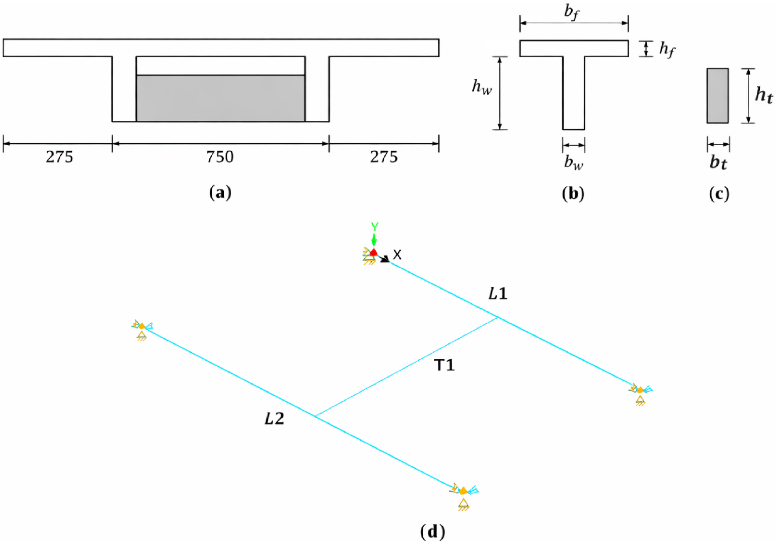

The mathematical model of the bridge (Figure 1(d)) consists of a pair of spars, L1 and L2, modeled like simply supported beams with a double T cross-section (Figure 1(b)) and a transverse beam T1 with a rectangular cross-section (Figure 1(c)).

To construct the mathematical model of the bridge, beams L1 and L2 were discretized with 50 spatial frame finite elements, with each element having a length of 20 cm. The transverse beam T1 was discretized with 1 spatial frame finite element having a length of 7.5 m. The complete model comprises 101 elements and 102 nodes. Regarding boundary conditions, it was assumed that the extremities of the beams L1 and L2 have 5 constraints, which include the displacement (all three axes) and rotation along the x and y-axis.

2.2. Mathematical model of the vehicle

The following vehicles analyzed are those that frequently travel on Brazilian highways, as observed by.^21,22 These vehicles are specifically 2C, 3C, and 2S3, as designated by the Brazilian National Department of Infrastructure and Transportation (DNIT). ²³ As illustrated in Figure 2(a), 2C and 3C are rigid trucks with two and three axles, respectively, while 2S3 is an articulated truck with five axles (two on the tractor and three on the trailer). The mathematical model of these vehicles consists of discrete systems formed by the association of masses, springs, and dampers, as illustrated in Figure 2(b).

Figure 2.

(a) Vehicles 2C, 3C, and 2S3; (b) Mathematical model of these vehicles.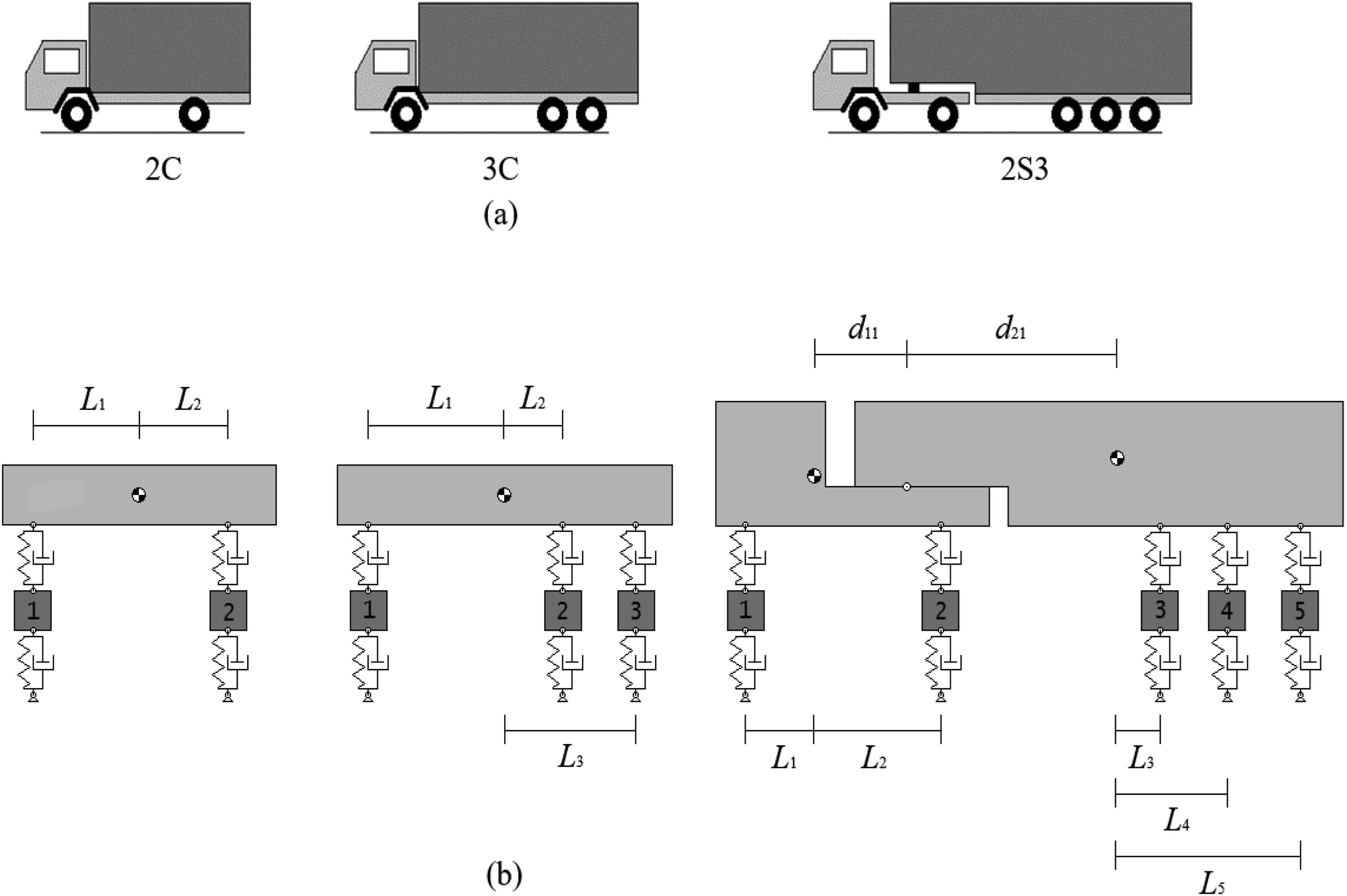

2.3. Mathematical model of the pavement

The following analyses considered two types of pavements: (i) a rough pavement generated according to the methodology outlined in ISO 8608, ²⁴ and (ii) a pavement that simulates an obstacle on the bridge entrance, generated following the methodology proposed by. ²⁵ In the next section, these two methodologies will be described in detail.

2.3.1. Rough pavement

To model the stochastic roughness profile of the pavement, the methodology outlined in ²⁴ was employed. To accomplish this, it is necessary to use a Power Spectral Density (PSD) function, as shown in the following expression:

$G_d\left(n\right)=G_d\left(n_0\right){\left(\frac{n}{n_0}\right)}^{-w}$

(1)

wherein $G_d\left(n\right)$ is the displacement PSD as a function of spatial frequency, in $m^3$ ; $G_d\left(n_0\right)$ is the reference PSD, in $m^3$ ; $n$ is the spatial frequency, which, according to, ²⁴ has a value in the range of [0.011, 2.83] cycles/m; $n_0$ is the reference spatial frequency, whose value is 0.1 cycles/m; and $w$ is the exponent of the PSD.

Regarding the reference PSD value, ISO 8608 ²⁴ classifies roads into eight categories, from A (new, nearly flat pavement) to H (poorly maintained, high-roughness pavement). For each class, the value of the geometric mean $G_d\left(n_0\right)$ is given in ²⁴ .

After evaluating $G_d\left(n\right)$ , the signal for pavement vertical displacement can be generated using the harmonic wave superposition method proposed by, ²⁶ and expressed in the following equation:

$u_{ir}\left(x\right)={\displaystyle \sum }_{k=1}^N\sqrt{2G_d\left(n_k\right)\Delta n}\mathit{cos}\left(2\pi n_{k}x+{\varphi }_k\right)$

(2)

in which $u_{ir}\left(x\right)$ is the pavement roughness elevation; $N$ is the number of frequency band intervals; $\mathrm{\Delta }n$ is the spatial frequency variation interval; $x$ is the position of the vehicle wheel on the road; $\varphi$ is the random, independent, and uniformly distributed in the range $\left[0,2\pi \right]$ phase angle.

For a 3D vehicle model numerical analysis, pavement roughness profiles must be generated for both sides of the vehicle. ISO 8608 ²⁴ allows assuming road surface isotropy, meaning profiles generated from one track share the same properties as the original, regardless of orientation or location.

If the pavement roughness profile on the vehicle’s right side is generated by equation (1) and isotropy hypothesis is true, a correlation exists between the left and right profiles. The PSD function for the left side is described by the equation ²⁷ :

$u_{ire}\left(x\right)={\displaystyle \sum }_{k=1}^N\left[\sqrt{2G_{de}\left(n_k\right)\Delta n}\mathit{cos}\left(2\pi n_{k}x+{\varphi }_k\right)+\sqrt{2\left[G_d\left(n_k\right)-G_{de}\left(n_k\right)\right]\Delta n}\mathit{cos}\left(2\pi n_{k}x+{\beta }_k\right)\right]$

(3)

in which $u_{ire}\left(x\right)$ is the pavement roughness elevation for the left side of the vehicle; $\beta$ is a random, independent, and uniformly distributed in a range of $\left[0,2\pi \right]$ phase angle; $G_{de}\left(n\right)$ is the cross-PSD function evaluated according to the expression:

$G_{de}\left(n\right)=\gamma \left(n\right)G_d\left(n\right)$

(4)

in which $\gamma \left(n\right)$ represents a coherency function for two PSDs for the spatial frequency $n$ .

According to, ²⁷ the function $\gamma \left(n\right)$ corresponds to the square module of a transfer function of a filter for frequencies of direct excitation. This variable is defined by the equation:

$\gamma \left(n\right)=\frac{v_l^2}{v_l^2+n^2}$

(5)

where $v_l$ is a cut-off frequency whose value was obtained experimentally and amounts to 0.2 cycles/m.

2.3.2. Pavement that represents an obstacle on the bridge entrance

Obstacles at the bridge entrance, such as potholes, expansion joints, or ledges, can be modeled using the expression proposed by. ²⁵ Both types of obstacles can be modeled using equation (6). What differs between each type of obstacle is the presence of a negative sign. That is, the depression (pothole) has a negative sign, whereas the ledge does not have this sign in its expression.

$u_{ir}\left(x\right)=\{\begin{array}{ll}-\frac{a}{2}\left[1-\mathit{cos}\left(\frac{2\pi x}{b}\right)\right],& 0\le x\le b\\ 0,& x<0\hspace{0.17em}or\hspace{0.17em}x>b\end{array}$

(6)

wherein $a$ is the pothole depth or the ledge height; $x$ is the position of the vehicle wheel; $b$ is the length of the pothole or the ledge.

When evaluating the length of a pothole or ledge, one should use the following expression:

$b=\frac{v}{f_n}$

(7)

in which $v$ is the vehicle velocity; $f_n$ is the first natural frequency of the bridge.

As the analyses are carried out with a three-dimensional model of the vehicles, in the case of a pavement that represents an obstacle, it does not necessarily correlate with the obstacle profile for each side of the vehicle. This paper considers that both sides of the vehicle travel along the same obstacle profile.

2.4. Optimization of TMD parameters

The focus of this paper is to propose a robust methodology for optimizing TMDs to reduce the vibration amplitude of bridges subjected to moving vehicles considering the uncertainties. In this manuscript, robustness refers to the design of the TMD parameters (mass, stiffness, and damping) such that their performance is not overly sensitive to the variations considered in bridge geometry and mechanical properties, pavement roughness, and vehicle parameters. In other words, the objective was to obtain a set of TMD parameters capable of delivering satisfactory performance across a range of plausible structural and operational conditions, rather than being optimal for a single deterministic configuration.

TMD parameters can be determined either through analytic equations (e.g.,^28,29 ) or meta-heuristic optimization algorithms. Studies developed by^10,17,20 showed that the latter yields the greatest reduction in structural vibration, making it the chosen method for designing the TMDs for the bridge analyzed here.

Among available meta-heuristic algorithms, the Honey Badger Algorithm (HBA) developed by ³⁰ was selected for its concise code, minimal input requirements, and clear steps for finding the global minimum. HBA converges quickly without the using many search agents and includes strategies to avoid entrapment in local minima.

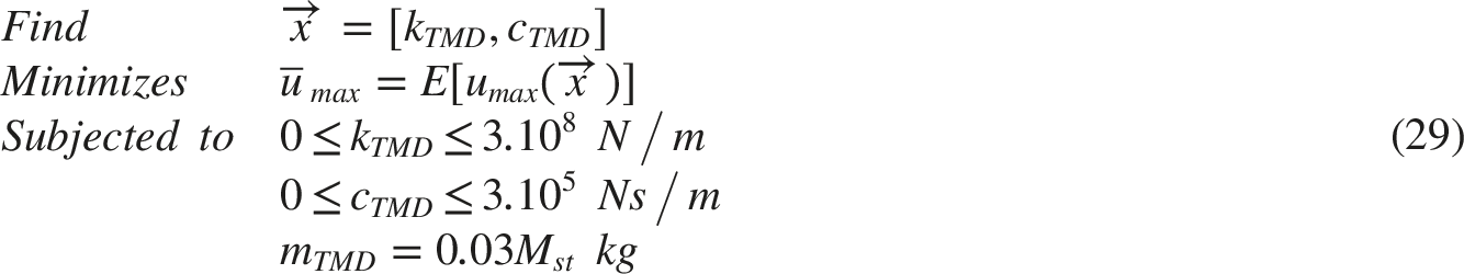
Therefore, the optimization problem that will be solved with the HBA algorithm is shown in the expression:

$\begin{array}{ll}Find& \overrightarrow{x}=\left[k_{TMD},c_{TMD}\right]\\ Minimizes& {\overline{u}}_{\mathit{max}}=E\left[u_{\mathit{max}}\left(\overrightarrow{x}\right)\right]\\ Subjected\hspace{0.17em}to& k_{TMD}^{\mathit{min}}\le k_{TMD}\le k_{TMD}^{\mathit{max}}\\ & c_{TMD}^{\mathit{min}}\le c_{TMD}\le c_{TMD}^{\mathit{max}}\\ & m_{TMD}=\eta M_{st}\end{array}$

(8)

in which, $\overrightarrow{x}$ denotes the design variables vector, $k_{TMD}$ is the TMD stiffness, $c_{TMD}$ is the TMD damping, $k_{TMD}^{\mathit{min}}$ and $k_{TMD}^{\mathit{max}}$ denote the bounds for TMD stiffness, while $c_{TMD}^{\mathit{min}}$ and $c_{TMD}^{\mathit{max}}$ are the bounds for TMD damping. The variable $\eta$ represents the percentage of structure mass (in general, varying in the range of 1% to 5% of the total mass of the structure ²⁰ ), $M_{st}$ is the total mass of the structure, and $u_{max}\left(\overrightarrow{x}\right)$ indicates the bridge’s maximum vertical displacement based on TMD parameters. $E\left[u_{\mathit{max}}\left(\overrightarrow{x}\right)\right]$ is the mean value of maximum displacement of the bridge over a number of samples, and ${\overline{u}}_{\mathit{max}}$ is the robust optimization objective function for the bridge’s mean maximum vertical displacement.

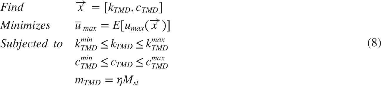
The adopted optimization framework is therefore risk-neutral. The objective function was defined as the minimization of the expected value (mean) of the maximum bridge displacement, computed through Monte Carlo simulation. No additional risk-averse robustness measures, such as variance minimization, quantile-based criteria, or reliability indices, were incorporated into the objective function. This choice was intentional, as the primary goal of the study was to reduce the average peak structural response while ensuring that the optimized TMD remains effective under the considered uncertainties.

More information about Monte Carlo simulations and the balance between robustness and computational tractability necessary to provide a practical and implementable strategy for stochastic TMD design are presented in the following sections of the manuscript.

2.5. Honey badger optimization algorithm (HBA)

The meta-heuristic algorithm HBA is inspired by the behavior of honey badgers during their food-finding process. In their natural environment, these behaviors include excavation (searching for food in the ground) or following honeybirds in search of beehives. ³⁰

According to, ³⁰ the computational implementation of the HBA algorithm is easy to do and, based on the working principle of the method, some evaluations are necessary to reach the minimum value of the objective function.

The first step in the computational implementation of the HBA algorithm involves initializing the positions of each honey badger (referred to as the search agents). This is accomplished using the following expression:

${\overrightarrow{x}}_i={\overrightarrow{lb}}_i+{\overrightarrow{z}}_1\left({\overrightarrow{ub}}_i-{\overrightarrow{lb}}_i\right),i=1,2,...,N_{sa}$

(9)

where ${\overrightarrow{x}}_i$ is a vector with the position of the i^th search agent; ${\overrightarrow{lb}}_i$ is a vector with the lower bound of the project variables; ${\overrightarrow{ub}}_i$ is a vector with the upper bound of the project variables; ${\overrightarrow{z}}_1$ is a vector with a random number between 0 and 1 for all project variables; $N_{sa}$ is the number of search agents.

After defining the position for each search agent, the next step consists of evaluating the objective function for each search agent and selecting the position ( ${\overrightarrow{x}}_{prey}$ ) that results in the minimum value for the objective function.

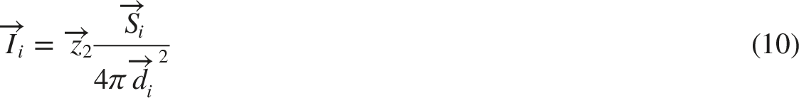
With this result, it is possible to evaluate the intensity, which measures how close the search agents are to the reference position and directs their movement. Intensity is evaluated according to the equation ³⁰ :

${\overrightarrow{I}}_i={\overrightarrow{z}}_2\frac{{\overrightarrow{S}}_i}{4\pi {\overrightarrow{d}}_i^2}$

(10)

${\overrightarrow{S}}_i={\left({\overrightarrow{x}}_i-{\overrightarrow{x}}_{i+1}\right)}^2$

(11)

${\overrightarrow{d}}_i={\overrightarrow{x}}_{prey}-{\overrightarrow{x}}_i$

(12)

wherein ${\overrightarrow{I}}_i$ is the intensity at which the i^th search agent will move; ${\overrightarrow{S}}_i$ is the concentration force factor of the i^th search agent; ${\overrightarrow{d}}_i$ is the distance between the prey and the i^th search agent; ${\overrightarrow{z}}_2$ is a vector with random numbers distributed between 0 and 1.

Besides that, the HBA algorithm uses a decreasing factor to smooth the transition between the exploration and exploitation phases and search for the response that minimizes the objective function. Such factor is evaluated as follows:

$\alpha =C\left[\mathit{exp}\left(\frac{-t}{t_{\mathit{max}}}\right)\right]$

(13)

where $\alpha$ is the decreasing factor; $t$ is the current iteration; $t_{\mathit{max}}$ is the maximum number of iterations; $C$ is a constant, whose amount is greater than 1.

Regarding the constant $C$ , by default, the amount is set to $C=2$ . This value was determined based on the sensitivity analysis conducted by, ³⁰ which showed that it resulted in the best performance of the algorithm during the search for the objective function minimum. Therefore, in the version of the HBA used in this study, the value of constant $C$ was kept as the default.

Finally, the update of the position of the search agents should be done with one of the following equations:

${\overrightarrow{x}}_{new}={\overrightarrow{x}}_{prey}+F\beta {\overrightarrow{I}}_i{\overrightarrow{x}}_{prey}+F{\overrightarrow{z}}_3\alpha {\overrightarrow{d}}_i\left|\cos \left(2\pi {\overrightarrow{z}}_4\right)[1-\cos \left(2\pi {\overrightarrow{z}}_5\right)]\right|, \text{if }{r}_1<0.5$

(14)

${\overrightarrow{x}}_{new}={\overrightarrow{x}}_{prey}+F{\overrightarrow{z}}_6\alpha {\overrightarrow{d}}_i, \text{if}\hspace{0.17em}{r}_1>0.5$

(15)

$F=\{\begin{array}{ll}1& if\hspace{0.17em}{r}_2\le 0.5\\ -1& otherwise\end{array}$

(16)

where ${\overrightarrow{x}}_{new}$ is the new position of the search agents; $F$ is a variable that allows the search agents to change their direction and escape for local minima; ${\overrightarrow{z}}_3$ , ${\overrightarrow{z}}_4$ , ${\overrightarrow{z}}_5$ , and ${\overrightarrow{z}}_6$ are vectors with random numbers between 0 and 1; $r_1$ and $r_2$ are random numbers between 0 and 1; $\beta$ is a factor that measures the capability of a search agent (honey badger) to find food.

The variable $\beta$ has also passed the sensitivity analysis of the algorithm’s performance. It was concluded that the amount that produces the best result in the search for the global minimum was $\beta =6$ , as reported by. ³⁰ For this reason, the variable $\beta$ was also maintained as the default value of the HBA algorithm during its use in the analysis performed in this work.

After updating the position of the search agents, the last step consists of verifying whether the new positions fall between the lower and upper bounds specified for the project variables. Then, the position that resulted in the lower value for the objective function is stored, and the entire process is repeated until the maximum number of iterations is completed.

2.6. Coupled system vehicle-bridge-pavement-TMD

Figure 3 presents a schematic drawing of the coupled vibration problem that is studied in this work.

Figure 3.

Description of the coupled system vehicle-bridge-pavement-TMD.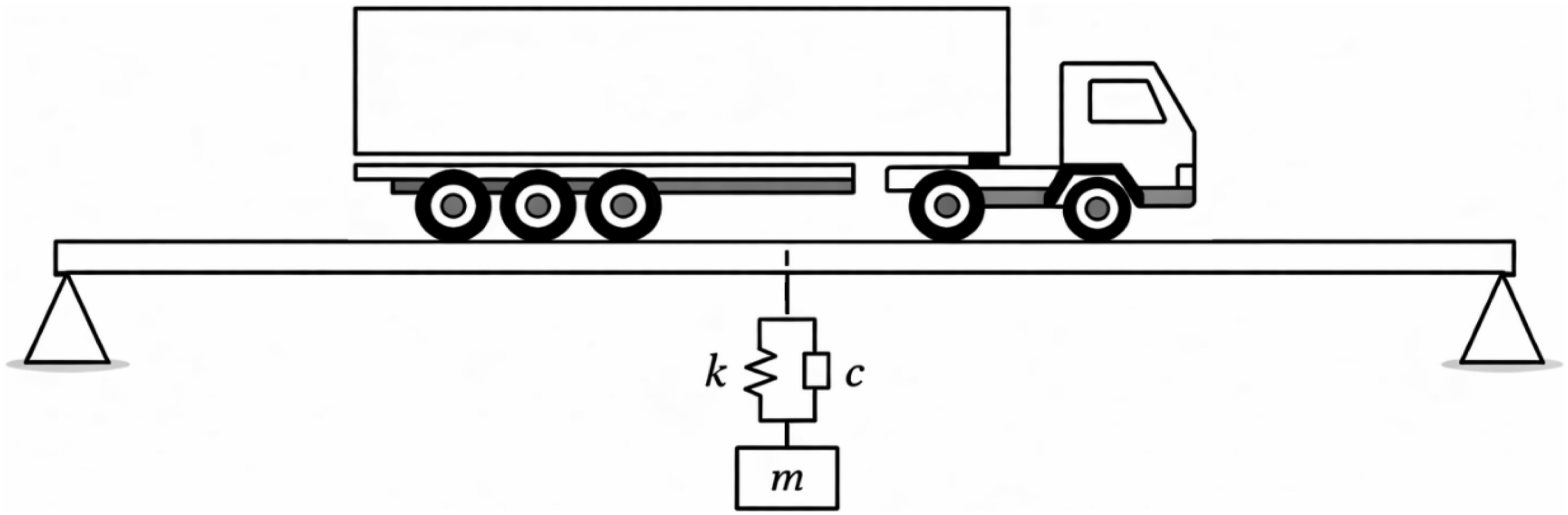

For this situation, the motion equation of the coupled system vehicle-bridge-pavement-TMD can be expressed as:

${\mathit{M}}_{VET}{\overrightarrow{\ddot{U}}}_{VET}+{\mathit{C}}_{VET}{\overrightarrow{\dot{U}}}_{VET}+{\mathit{K}}_{VET}{\overrightarrow{U}}_{VET}={\overrightarrow{F}}_{VET}$

(17)

where ${\mathit{M}}_{VET}$ , ${\mathit{C}}_{VET}$ , and ${\mathit{K}}_{VET}$ are the global matrices of mass, damping, and stiffness, respectively of the coupled system vehicle-bridge-pavement-TMD; ${\overrightarrow{F}}_{VET}$ is the global vector of forces due to the roughness of the pavement acting on the vehicle, bridge, and TMD; ${\overrightarrow{\ddot{U}}}_{VET}$ , ${\overrightarrow{\dot{U}}}_{VET}$ , and ${\overrightarrow{U}}_{VET}$ are the global vectors of acceleration, velocity, and displacement, respectively, of the coupled system vehicle-bridge-pavement-TMD.

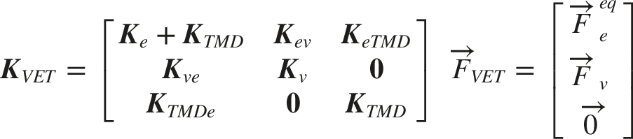
The matrices ${\mathit{M}}_{VET}$ , ${\mathit{C}}_{VET}$ , and ${\mathit{K}}_{VET}$ and the vector of forces of the equation (17) can be expressed as shown:

${\mathit{M}}_{VET}=\left[\begin{array}{lll}{\mathit{M}}_e& \mathbf{0}& \mathbf{0}\\ \mathbf{0}& {\mathit{M}}_v& \mathbf{0}\\ \mathbf{0}& \mathbf{0}& {\mathit{M}}_{TMD}\end{array}\right]\hspace{0.17em}{\mathit{C}}_{VET}=\left[\begin{array}{ccc}{\mathit{C}}_e+{\mathit{C}}_{TMD}& {\mathit{C}}_{ev}& {\mathit{C}}_{eTMD}\\ {\mathit{C}}_{ve}& {\mathit{C}}_v& \mathbf{0}\\ {\mathit{C}}_{TMDe}& \mathbf{0}& {\mathit{C}}_{TMD}\end{array}\right]$

(18)

${\mathit{K}}_{VET}=\left[\begin{array}{ccc}{\mathit{K}}_e+{\mathit{K}}_{TMD}& {\mathit{K}}_{ev}& {\mathit{K}}_{eTMD}\\ {\mathit{K}}_{ve}& {\mathit{K}}_v& \mathbf{0}\\ {\mathit{K}}_{TMDe}& \mathbf{0}& {\mathit{K}}_{TMD}\end{array}\right]\hspace{0.17em}{\overrightarrow{F}}_{VET}=\left[\begin{array}{l}{\overrightarrow{F}}_e^{eq}\\ {\overrightarrow{F}}_v\\ \overrightarrow{0}\end{array}\right]$

wherein ${\mathit{M}}_e$ , ${\mathit{C}}_e$ , and ${\mathit{K}}_e$ represent the mass, damping, and stiffness matrices of the bridge; ${\mathit{M}}_v$ , ${\mathit{C}}_v$ , and ${\mathit{K}}_v$ represent those of the vehicle; ${\mathit{M}}_{TMD}$ , ${\mathit{C}}_{TMD}$ , and ${\mathit{K}}_{TMD}$ correspond to the TMDs. ${\mathit{C}}_{ev}$ , ${\mathit{C}}_{ve}$ , ${\mathit{K}}_{ev}$ , and ${\mathit{K}}_{ve}$ relate to the damping and stiffness of the vehicle’s tires interacting with the bridge’s vertical displacement and updating with wheel changes. ${\mathit{C}}_{TMDe}$ , ${\mathit{C}}_{eTMD}$ , ${\mathit{C}}_{TMDe}$ , and ${\mathit{K}}_{eTMD}$ are the damping and stiffness matrices of the TMDs interacting with the bridge’s vertical displacement. ${\overrightarrow{F}}_e^{eq}$ is the vector of equivalent loads on the bridge, ${\overrightarrow{F}}_v$ is the vector of forces on the vehicle, and $\mathbf{0}$ and $\overrightarrow{0}$ represent a null matrix and a null vector, respectively.

It is important to highlight that the damping matrix of the structure was evaluated using the Rayleigh damping methodology ³¹ and was assumed to be proportional to the stiffness matrix and the first natural frequency. A critical damping ratio of 3% was adopted for the first vibration mode of the structure.

The forces acting on the bridge and the vehicle vary according to the pavement elevation and the vehicle’s position inside the bridge. The local vector forces acting on the vehicle and the bridge should be evaluated according to the expressions^2,10,17:

${\overrightarrow{F}}_v=f_{ir},\text{for}\hspace{0.17em}j=1,2,...,N_{wheels}$

(19)

${\overrightarrow{F}}_e=-\left[f_{ir}+\left(m_{pj}+W_j{m}_s\right)g\right],\text{for}\hspace{0.17em}j=1,2,...,N_{wheels}$

(20)

$f_{ir}=c_{pj}{\dot{u}}_{ir}+k_{pj}{u}_{ir}$

(21)

in which $m_{pj}$ , $c_{pj}$ , and $k_{pj}$ are the mass, damping, and stiffness of the j^th vehicle’s tire; $u_{ir}$ is the pavement roughness elevation; ${\dot{u}}_{ir}$ is the derivative with respect to time of the pavement roughness elevation; $m_s$ is the vehicle’s sprung mass; $W_j$ is the percentage of sprung mass that is transferred for each wheel; $g$ is the gravity acceleration, whose amount is 9.81 m/s²; $N_{wheels}$ is the vehicle’s number of wheels.

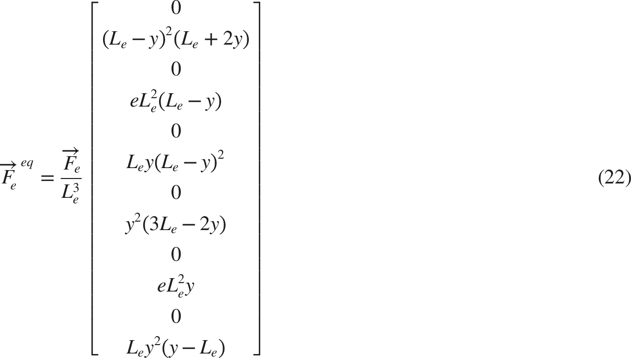
Because of factors like finite element discretization, vehicle speed, and the time step for integrating the motion equation, the vehicle’s wheel contact points may not align with the bridge model nodes at a given time. This misalignment means the pavement roughness force isn’t directly applied to the bridge’s force vector. In such cases, equivalent nodal forces must be calculated and applied to the bridge elements, as given by the spatial frame finite element expression ³² :

${\overrightarrow{F}}_e^{eq}=\frac{{\overrightarrow{F}}_e}{L_e^3}\left[\begin{array}{c}0\\ {\left(L_e-y\right)}^2\left(L_e+2y\right)\\ 0\\ e{L}_e^2\left(L_e-y\right)\\ 0\\ L_{e}y{\left(L_e-y\right)}^2\\ 0\\ y^2\left(3L_e-2y\right)\\ 0\\ e{L}_e^{2}y\\ 0\\ {L_{e}y}^2\left(y-L_e\right)\end{array}\right]$

(22)

where ${\overrightarrow{F}}_e$ is the force vector that rough pavement and the vehicle caused in the bridge, evaluated with equation (20); $L_e$ is the length of the spatial frame finite element; $y$ is the distance from the left node of the element to the point where the force is applied; $e$ is the distance of the bridge’s axis to the vehicle’s wheels.

The integration of the motion equation to obtain the displacements of the bridge is carried out using Newmark’s Method. The entire methodology presented in this section was computationally implemented using the Octave language.

2.7. Computational implementation of the problem

To carry out the analyses proposed in this paper, a computational code was developed using the Octave programming language. The choice of this programming language was driven by several reasons: it is open source, its syntax is very similar to MATLAB, and it supports code parallelization.

The computational code developed consists of nine subroutines, each handling a specific part of the methodology, and a main program that uses these subroutines to process input data and display analysis results. The organization of the main program is illustrated in the flowchart in Figure 4.

Figure 4.

Flowchart of the main program.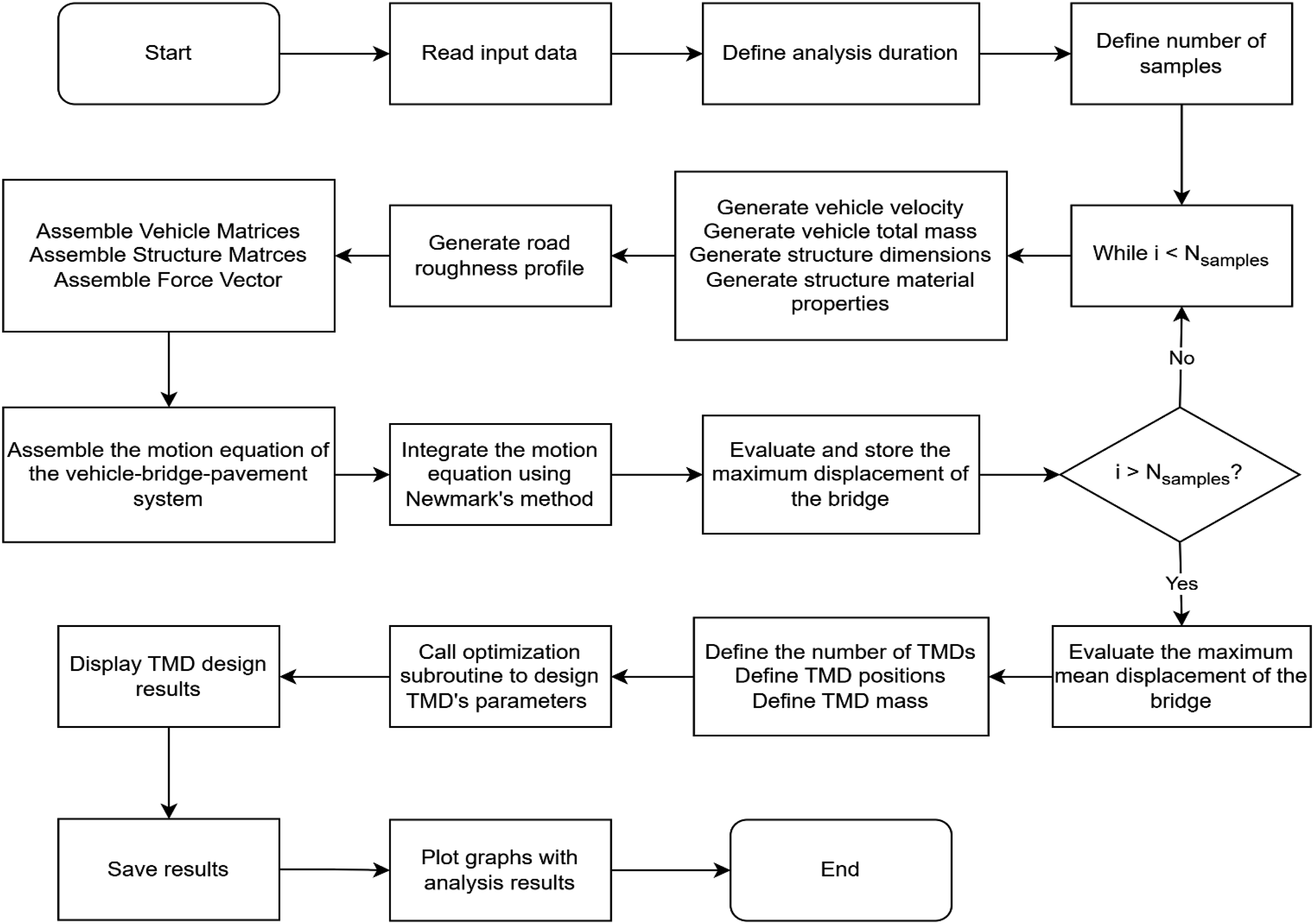

TMD design for the bridge uses robust optimization, requiring the objective function to be evaluated across multiple samples of the problem’s random variables. For each sample, the bridge’s maximum displacement is calculated, and these results are averaged to determine the objective function value for the optimization.

Since the maximum displacement of the bridge needs to be evaluated multiple times for each sample, there is potential to save computational time by parallelizing this portion of the code. In this context of engineering practice, several widely used computational procedures are naturally suited for parallelization. Finite Element Analysis (FEA), Monte Carlo Simulation (MCS), Computational Fluid Dynamics (CFD), and broader Computer-Aided Engineering (CAE) workflows often involve either domain decomposition strategies or repeated independent simulations.

The adoption of parallel processing in common engineering design environments has become increasingly feasible due to advances in modern computing hardware. Contemporary workstations are typically equipped with multi-core CPUs and, in many cases, graphics processing units (GPUs), which enable efficient parallel execution of computational tasks without requiring specialized high-performance computing infrastructure.

The practical benefits of parallel processing in design settings include significant reduction in computational time, improved utilization of available hardware resources, and increased feasibility of conducting large parametric studies or stochastic analyses within standard project deadlines. By reducing turnaround time, engineers can evaluate a greater number of design alternatives, perform more comprehensive sensitivity analyses, and improve the robustness of the final solution. The parallelization process used in this work is explained in the next section.

2.7.1. Parallelization of the objective function evaluation

In contrast to languages like C/C++ and Fortran, which use OpenMP (Open Multi-Processing) interface for code parallelization, Octave relies on specialized external packages, such as the parallel, MPI, and Dragonfly packages.^33,34

This paper utilizes the parallel package, developed by H. Fujiwara, J. Hajek, and O. Till, ³⁵ for the application of parallelization. This package provides a set of functions that can be used within Octave scripts. Additionally, these functions can be executed on local machines with shared memory as well as on clusters with distributed memory. ³⁴

In Octave’s parallel package, we use the “pararrayfun” function to execute code on a local machine with multiple processors and shared memory. It requires three arguments: (i) the number of processors, (ii) the name of the Octave function, and (iii) a vector of arguments for the function. ³⁶ An example of syntax is shown in equation (23).

$\left[o_1,o_2,\dots \right]=pararrayfun\left(N_{proc},fun,a_1,a_2,\dots \hspace{0.17em}\right)$

(23)

where, $o_1$ and $o_2$ are the outputs of the function; $N_{proc}$ is the number of processors available in the machine; $fun$ is the Octave function (file with extension .m); $a_1$ and $a_2$ are the arguments of the function.

Parallelization was applied to the objective function evaluations during optimization to reduce computational time. Since the maximum displacement needed to be evaluated for all samples, this code section was divided among the machine’s processors for simultaneous execution, leading to a significant reduction in evaluation time.

It is important to note that the program developed in this paper for the design of TMDs or MTMDs, aimed at reducing the dynamic response of the bridge for the considered vehicles, was executed on a machine equipped with 8 Intel Xeon E5-4685 processors, each with 12 cores running at 2.70 GHz, 488 GB of RAM, and the Debian Linux 10 operating system.

The flowchart detailing the operations executed within the parallel subroutine to calculate the objective function value is shown in Figure 5.

Figure 5.

Flowchart detailing the parallelization applied in the optimization process and the operations performed to evaluate the objective function.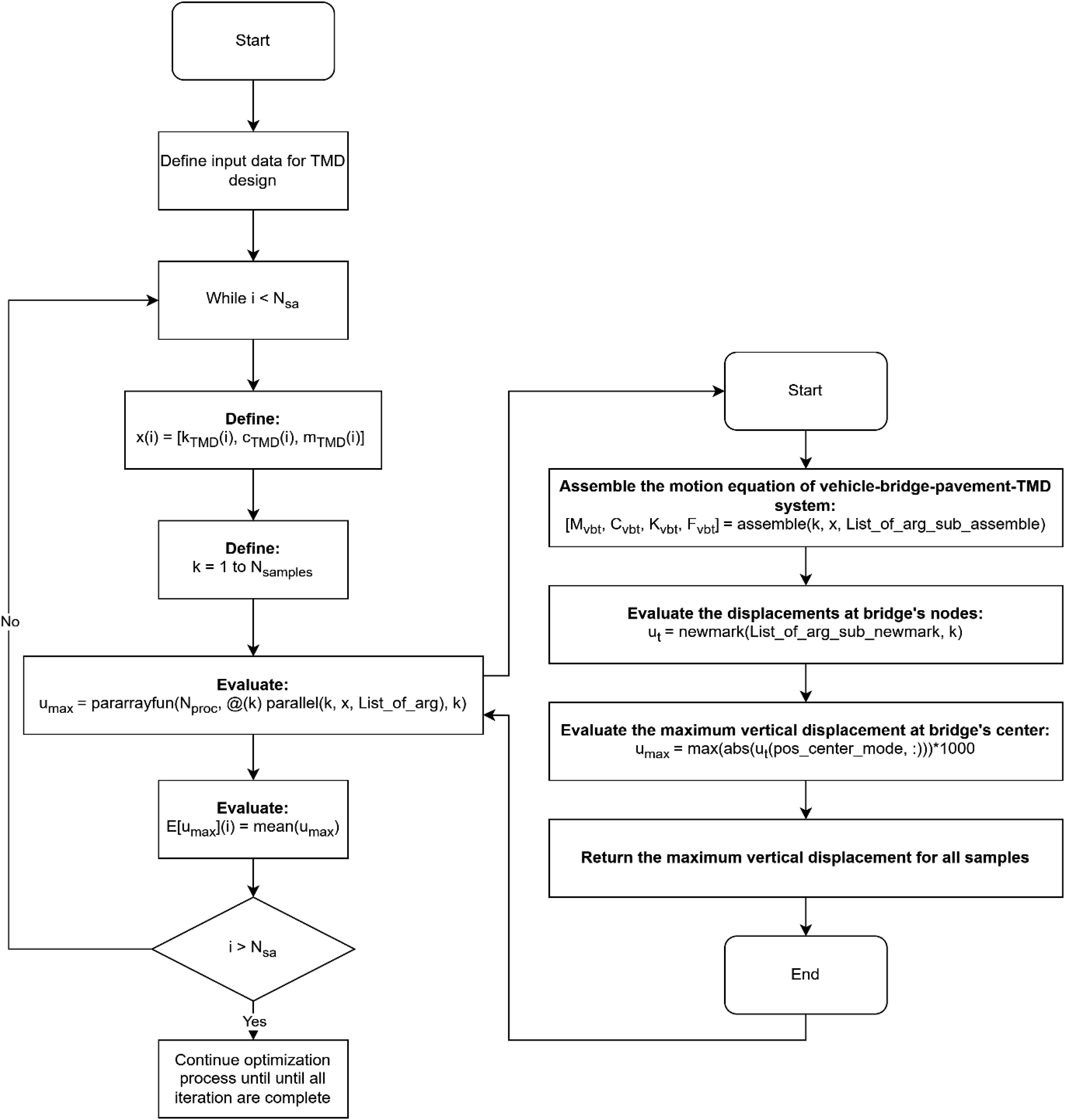

3. Results and discussions

3.1. Uncertainties considered on the structure, vehicle, and pavement

The optimization problems in this work account for inherent uncertainties in both the structure and vehicle properties, making each vehicle-bridge-pavement-TMD simulation yield a unique bridge displacement and resulting in a stochastic system response.

Regarding the structure, it was considered that uncertainties lie in the dimensions of the cross-section of beams L1, L2, and T1 as well as their material properties, specifically elasticity modulus ( $E$ ) and density ( $\rho$ ). The uncertainties in the dimensions of the beams follow a normal distribution, with the mean value representing the nominal dimensions of the beam’s cross-section and the standard deviation representing construction tolerances according to the Brazilian code NBR 14931:2023. ³⁷

The dimensions used to generate the beam cross-sections follow a normal distribution with specific means and standard deviations: 30 cm ( $b_w$ ), 75 cm ( $h_w$ ), 25 cm ( $h_f$ ), 30 cm ( $b_t$ ), and 60 cm ( $h_t$ ), with standard deviations of 0.5 cm, 0.7 cm, 0.5 cm, 0.5 cm, and 0.5 cm, respectively. As these uncertainties are on the dimensions of the beams, the proper computational code was developed to evaluate the inertia moments used to assemble the global matrices of the mathematical model of the bridge.

The variable $b_f$ , which represents the length of the flange in a T-shaped beam (Figure 1(b)), is defined as the length in which a reinforced concrete piece has a uniform compression stress distribution according to the Brazilian code NBR 6118:2023. ³⁸ However, it is also a random variable, but its values are evaluated as a function of the base of the beam ( $b_w$ ) and the span of the bridge ( $L$ ), as shown in the equation:

$b_f=b_w+\frac{L}{5}$

(24)

When it comes to the variables associated with the properties of the bridge material, we assume that the uncertainties are correlated. The generation of these uncertainties should be carried out using equation (25). ³⁹ For the relevant variables, we consider the following values: an elastic modulus of 30 GPa, with a standard deviation of 3 GPa and a correlation coefficient of 0.8; and for density, we have values of 2,500 kg/m³, a standard deviation of 250 kg/m³, and a correlation coefficient of 0.8 as well.

$\left[\begin{array}{l}E\\ \rho \end{array}\right]=\left(\mathit{L}\mathit{S}\right)\overrightarrow{Z}+{\overrightarrow{\mu }}_X$

(25)

in which $\mathit{L}$ is the lower triangular of Cholesky’s factorization of the matrix with correlation coefficients of the random variables; $\mathit{S}$ is a matrix with the standard deviation of the random variables; $\overrightarrow{Z}$ is a vector with random numbers uniformly distributed between 0 and 1; ${\overrightarrow{\mu }}_X$ is a vector with the mean values of the random variables.

The matrices with the correlation coefficients ( $\mathit{R}$ ) and with the standard deviation ( $\mathit{S}$ ) of the random variables are defined according to the expressions:

$\mathit{R}=\left[\begin{array}{cc}1& Cor\left(E,\rho \right)\\ Cor\left(\rho ,E\right)& 1\end{array}\right]\hspace{0.17em}\mathit{S}=\left[\begin{array}{ll}{\sigma }_E& 0\\ 0& {\sigma }_{\rho }\end{array}\right]$

(26)

where $Cor\left(E,\rho \right)$ and $Cor\left(\rho ,E\right)$ are the values of the correlation of $E$ regarding $\rho$ and $\rho$ regarding $E$ , respectively; ${\sigma }_E$ is the standard deviation of the elasticity modulus; ${\sigma }_{\rho }$ is the standard deviation of density.

For the vehicles, the uncertainties considered are the total masses, velocities, and axle spacing. It should be noted that no uncertainties are incorporated into the values for the tires and suspension systems.

For a single tire, the mass, stiffness, and damping are 320 kg, 840 kN/m, and 1 kNs/m. For a double tire, they are 530 kg, 1,680 kN/m, and 2 kNs/m. The suspension system’s characteristics are 290 kN/m and 3 kNs/m for single tires, and 590 kN/m and 6 kNs/m for double tires.

Axle spacing data for the vehicles was sourced from, ⁴⁰ based on dimensions observed on Brazilian highways. The methodology referenced from ⁴¹ employs a Beta distribution to determine vehicle spacing in the same lane. Using this distribution along with the maximum and minimum axle spacing values, the dimensions of each vehicle were generated. Relevant data is presented in Table 1.

Table 1.

Range values for axle spacing, probability function, percentage of sprung mass transferred to each axle, and tire type.

Vehicle	Axle spacing (m)	Distribution	W (%)	Tire type
	[3.30; 14.33]	Beta	25	Single
			75	Double
			​	​
	[2.67; 15.10]	Beta	22.6	Single
	1.30	-	38.7	Double
	​	​	38.7	Double
	​	​	​	​
	[2.44; 6.50]	Beta	14.2	Single
	[5.00; 10.40]	Beta	30.6	Double
	1.25	-	18.4	Double
	1.25	-	18.4	Double
	​	​	18.4	Double

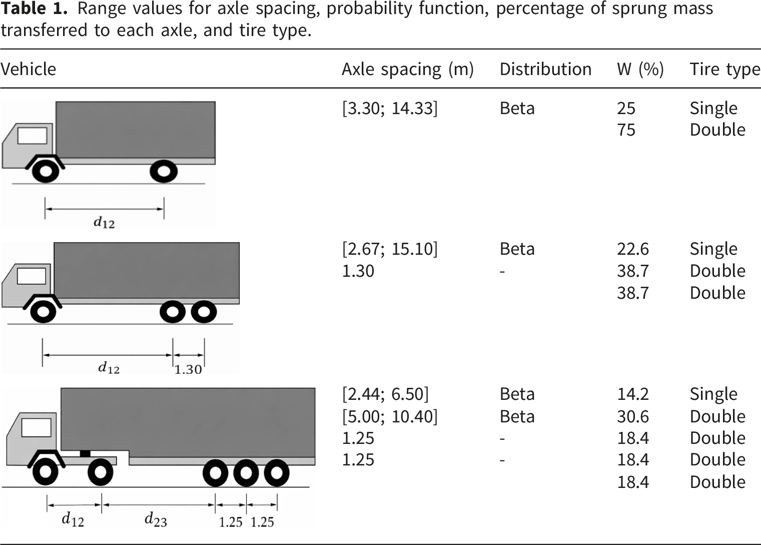
It is important to emphasize that the position of the mass center of the vehicles and the distances from this point to the axles are evaluated for the developed computational program with respect to the generated axle spacing and the spung mass percentage transferred to each axle.

The mass of vehicles follows a normal distribution based on data from. ⁴¹ Vehicle 2C has a mean mass of 19,500 kg and a standard deviation of 3,400 kg, while vehicle 3C has a mean mass of 25,700 kg and a standard deviation of 4,300 kg. For vehicle 2S3, the tractor unit weighs 9,000 kg, and the trailer has a mean mass of 46,300 kg with a standard deviation of 7,900 kg.

When assembling the vehicle model’s mass matrix, both the sprung mass and tire masses are considered. The total mass of the vehicle, treated as a random variable, is the sum of these masses, with only the sprung mass being variable. The total mass is generated first, followed by the determination of the sprung mass, as shown in equation (27). This variability, along with the stochastic nature of axle spacing, makes the moments of inertia random variables, which are calculated by the developed computational program.

$m_s=m_{total}-\left(N_{ps}{m}_{ps}+N_{pd}{m}_{pd}+m_{cv}\right)$

(27)

wherein $m_s$ is the sprung mass of the vehicle; $m_{total}$ is the total mass of the vehicle; $N_{ps}$ and $N_{pd}$ are the number of single and double tires, respectively; $m_{ps}$ and $m_{pd}$ are the masses of the single and double tires, respectively; $m_{cv}$ is the vehicle 2S3 tractor unity mass.

The vehicle velocities are generated using a normal distribution with a specified mean value and standard deviation. According to, ⁴⁰ the mean velocity for vehicles 2C and 3C is 77 km/h, with a standard deviation of 13.5 km/h. For vehicle 2S3, the mean velocity is 78 km/h, with a standard deviation of 11 km/h.

Regarding the uncertainties considered in the pavement when the bridge’s pavement is rough, the methodology used to convert the signal from frequency to time domain through a random phase angle was taken into consideration. For the pavement that simulates an obstacle at the entrance of the bridge, it was assumed that this pavement will contain a pothole. The uncertainties in this case lie in its depth, varying uniformly between 1 cm and 5 cm, and in its length, which is dependent on the velocity of the vehicle and the first natural frequency of the bridge, both of which are random variables as explained previously.

For all the analyses conducted, the vehicles were positioned on the right side of beam L1, with their axles set at distances of 15 cm and 235 cm from the axis of beam L1. An integration time step of 0.001 seconds was utilized for integrating the motion equation, and the total duration of the analysis was 1.71 seconds.

3.2. Convergence curves and sample number

To address uncertainties in the structure, vehicles, and pavement, it is essential to determine the number of samples needed to stabilize the maximum mean displacement at the bridge’s central node while minimizing computational costs, thereby ensuring statistical convergence of the expected response used in the optimization process and consistency with the adopted risk-neutral framework.

To evaluate it, static (without the force due to the pavement) and dynamic (with the force due to the pavement) analyses were conducted for each vehicle, considering two scenarios: (i) a bridge with class C rough pavement and (ii) a bridge with a pothole at its entrance. For all analyses, 600 samples of the variables presented in Section 3.1, and pavement profiles were generated for each scenario.

As a result, the convergence curve of the mean and variance of the maximum vertical displacement of at the center of the bridge for two situations considered was obtained, as shown in Figures 6 and 7, respectively. In the legend of the figures, “Dyn” means the dynamic analysis and “Static” represents the static analysis.

Figure 6.

Convergence curves of mean (upper) and variance (lower) of the maximum vertical displacement of the bridge for the situation (i) that considers rough pavement.

Figure 7.

Convergence curves of mean (upper) and variance (lower) of the maximum vertical displacement of the bridge for the situation (ii) that considers the pothole as a pavement.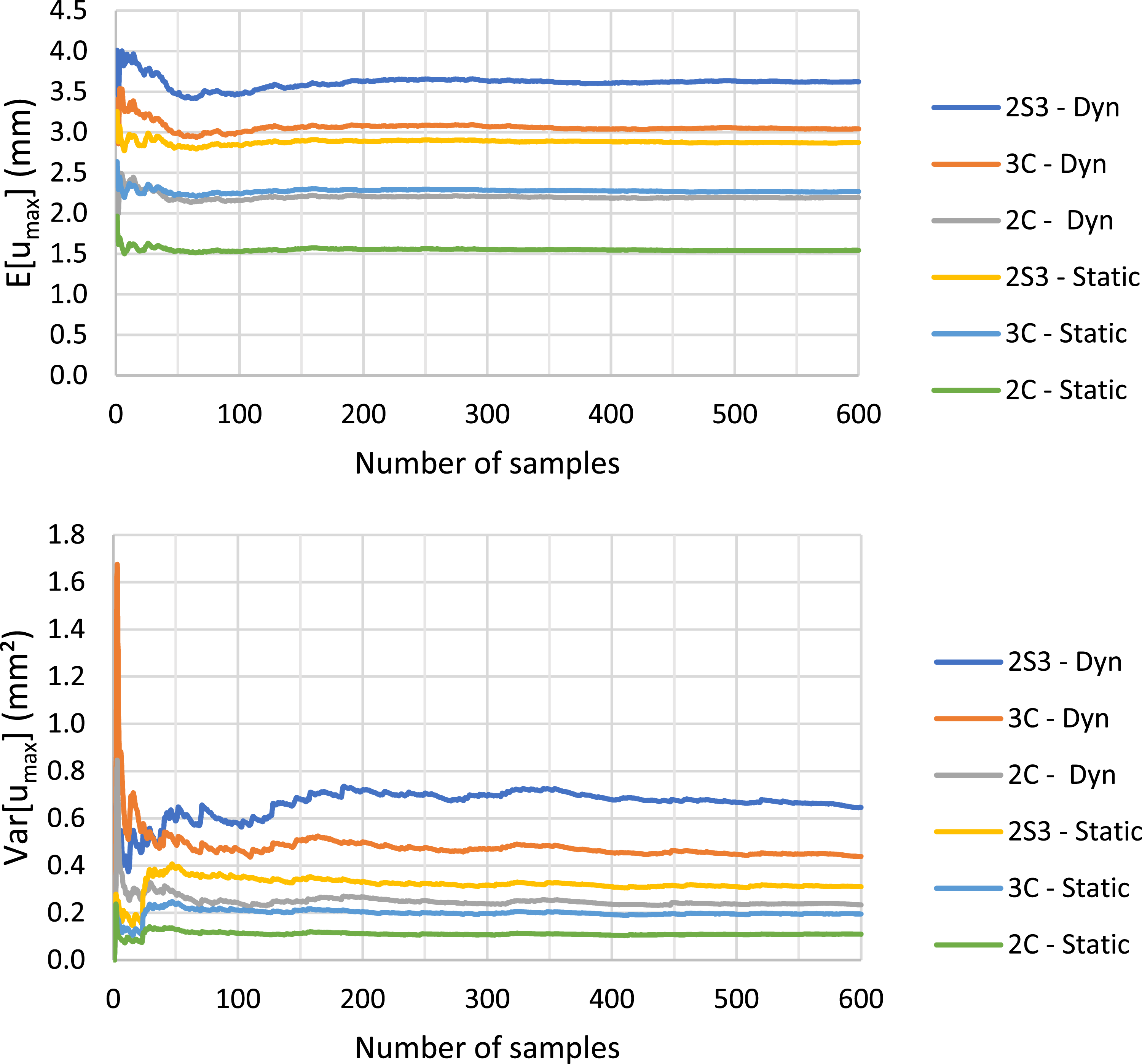

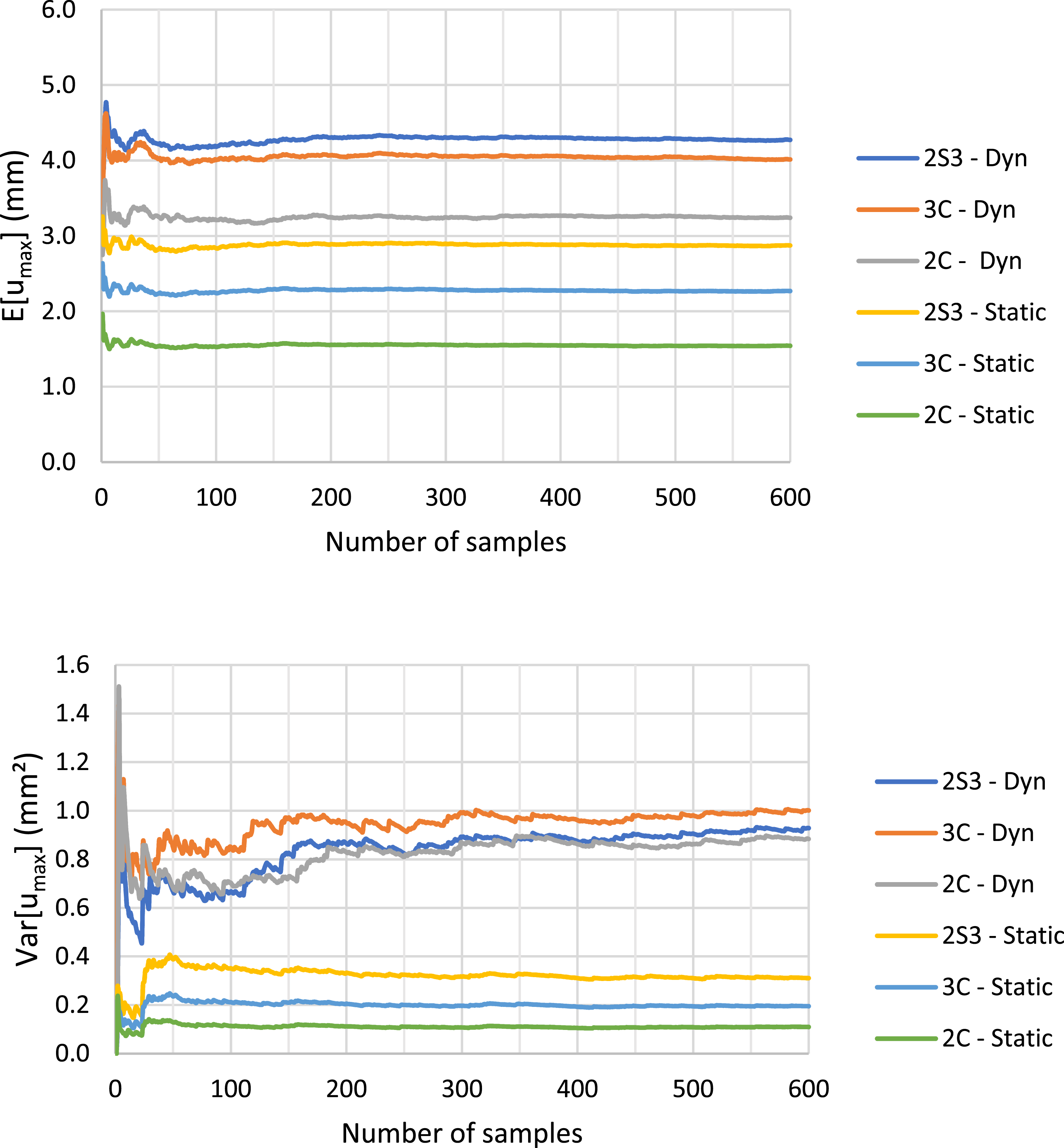
In Figures 6 and 7, it is notable that for the analyses with class C roughness and the pothole, both convergence curves became steady at about 250 samples. Therefore, the number of samples used for solving this optimization problem is 250.

Additionally, evaluating the ratio between the dynamic and static responses for the previously defined number of samples resulted in the Dynamic Amplification Factor (DAF) of the bridge. ⁴² In this study, this factor is treated as a statistical quantity, since the analysis incorporates stochastic variables within a Monte Carlo framework. Each realization produces distinct dynamic and static maximum displacements, and consequently a different amplification value. The reported result therefore corresponds to the mean value obtained across all samples. Consistent with the objectives of this work, the amplification is evaluated based on the mean maximum displacement of the bridge across all realizations, rather than on its extreme value.

These results are presented in Table 2, and the values were compared with the Vertical Impact Coefficient ( $Civ$ ), defined by the equation from the Brazilian moving loads code NBR 7188:2024, ⁴³ described as follows:

$Civ=\{\begin{array}{l}1.35,if\hspace{0.5em}L\le 10\hspace{0.17em}m\\ 1+1.06\left(\frac{20}{L+50}\right),if\hspace{0.5em}L>10\hspace{0.17em}m\end{array}$

(28)

where $L$ is the span of the bridge when the structure is simply supported.

Table 2.

Results for the static and dynamic maximum vertical displacement at the center of the bridge for situations (i) and (ii), and for each vehicle.

Pavement	Class C roughness			Pothole
Vehicle	2C	3C	2S3	2C	3C	2S3
Static (mm)	1.5433	2.2688	2.8731	1.5433	2.2688	2.8731
Dynamic (mm)	2.1928	3.0401	3.6217	3.2403	4.0129	4.2726
DAF	1.42	1.34	1.26	2.10	1.77	1.49
$Civ$	1.35	1.35	1.35	1.35	1.35	1.35

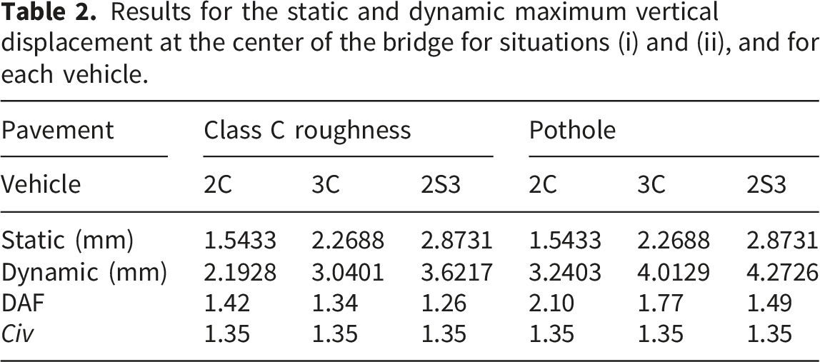
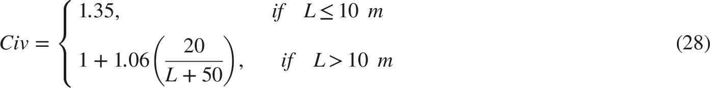
It is important to highlight that code-based impact coefficients are typically formulated as conservative design envelopes. In most bridge design standards, these coefficients are estimated as functions of structural characteristics, such as span length and natural frequency, and are applied to amplify variable loads in order to perform equivalent static analyses for design purposes. ⁴²

For instance, the Brazilian standard ABNT NBR 7188:2024 ⁴³ adopts this approach. It defines amplification coefficients to increase the magnitude of moving loads, including the $Civ$ , which has a similar physical interpretation to the DAF. However, these coefficients are intentionally conservative and are not intended to represent statistical mean responses.

The results in Table 2 show that the DAF of dynamic responses exceeded the $Civ$ specified by ⁴³ only for the 2C vehicle when the bridge pavement is rough. For the 3C and 2S3 vehicles, DAF values were below the limit, indicating that a TMD is not needed to reduce maximum bridge displacement for these vehicles.

Potholes in the pavement notably affect the bridge’s dynamic responses. Rigid vehicles, such as 2C and 3C, significantly increase the bridge’s dynamic response, while articulated vehicles like 2S3 show a smaller increase. Thus, for this pavement type, a TMD should be proposed to reduce the bridge’s dynamic response below the $Civ$ recommended by. ⁴³

3.3. Definition of the number of processors to use in the parallelization

A parallel version of the computational code was used on a computer with 192 processors to design the TMDs on the bridge for reducing vehicle-induced displacements. However, as noted in Section 3.2, achieving a stable result for maximum bridge displacement requires 250 samples. Thus, using all processors may not enhance performance compared to the sequential version.

Tests were performed using sequential and parallel versions of the computational code to determine the optimal number of processors for minimizing computation time in TMD design. The tests measured the time taken to evaluate the maximum displacement of the bridge across 250 random variable samples and to compute the objective function in the optimization process.

In the parallel version of the code, these evaluations were conducted using 8, 12, 24, and 64 processors. The computational times obtained for each processor configuration were then compared with the time taken to execute the sequential version of the code. The results are presented in the graph shown in Figure 8 and summarized in Table 3.

Figure 8.

Comparison of the computational time to evaluate the objective function of the optimization process with the sequential and parallel versions of the developed code.

Table 3.

Computational time to evaluate the objective function for the sequential and parallel versions of the code.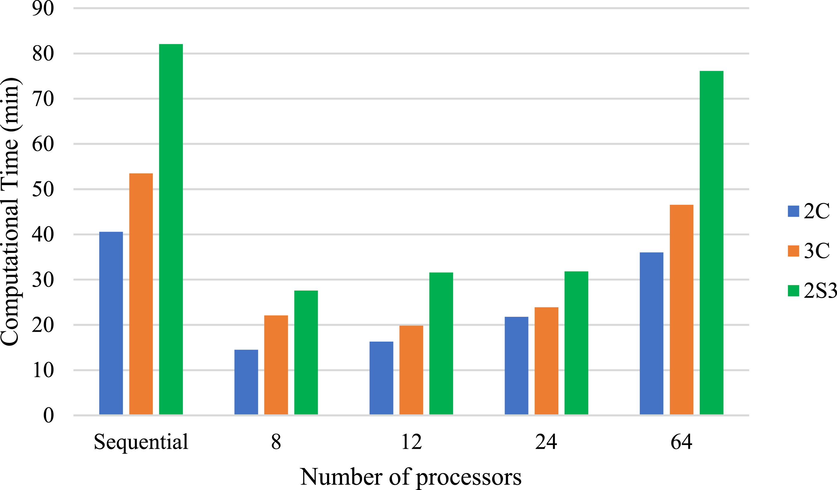

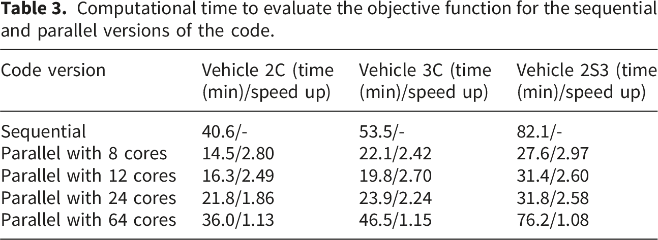
Code version	Vehicle 2C (time (min)/speed up)	Vehicle 3C (time (min)/speed up)	Vehicle 2S3 (time (min)/speed up)
Sequential	40.6/-	53.5/-	82.1/-
Parallel with 8 cores	14.5/2.80	22.1/2.42	27.6/2.97
Parallel with 12 cores	16.3/2.49	19.8/2.70	31.4/2.60
Parallel with 24 cores	21.8/1.86	23.9/2.24	31.8/2.58
Parallel with 64 cores	36.0/1.13	46.5/1.15	76.2/1.08

From the results shown in Figure 8 and Table 3, it can be observed that using 8 or 12 processors provides the best performance for the parallel version of the code. Therefore, all the primary analyses conducted in this study were performed using the parallel version with either 8 or 12 processors.

Simulations performed with 64 processors exhibited performance comparable to that of the sequential implementation, primarily due to the relatively small number of samples required to achieve steady estimates of the bridge displacement. The increased memory demand associated with the use of a large number of processors resulted in diminished efficiency, leading to better overall performance when fewer processors were employed in the parallel implementation.

The parallel implementation using 8 or 12 processors achieved a reduction in computational time of approximately 60% for all analyzed vehicles, compared to the sequential version, for a single evaluation of the objective function during the optimization process. This substantial improvement motivated the adoption of the parallel version for the TMD design optimization.

3.4. Design of one TMD for the bridge with rough pavement

Table 2 shows that the maximum mean vertical displacement at the center of the bridge exceeded the limit from ⁴³ only for vehicle 2C under rough pavement class C. Vehicles 3C and 2S3 stayed within the limit, indicating that a TMD is not needed for these vehicles.

The article discusses the design of TMDs for controlling bridge vibrations caused by vehicle loads. It outlines the implementation of a TMD, regardless of necessity, for all considered vehicles to showcase the proposed methodology’s effectiveness. To minimize the bridge’s maximum mean displacement, a TMD will be centrally installed and designed using the HBA optimization algorithm for each vehicle.

The reason TMD is centrally installed is that the bridge considered in the analysis is simply supported, and, in dynamic analysis, the first vibration mode is predominant, with its maximum amplitude at the center of the span for this type of structure. For that, it was opted to place the TMD at the center of the bridge and to design its parameters to match the structure’s first natural frequency as closely as possible.

The optimization problem, defined by equation (29), aimed to minimize the maximum mean vertical displacement of the bridge by searching for TMD parameters. This was achieved using 10 search agents, 25 iterations, and 250 samples of random variables, with a parallel code running on 12 processors. The TMD design results are shown in Table 4.

$\begin{array}{ll}Find& \overrightarrow{x}=\left[k_{TMD},c_{TMD}\right]\\ Minimizes& {\overline{u}}_{\mathit{max}}=E\left[u_{\mathit{max}}\left(\overrightarrow{x}\right)\right]\\ Subjected\hspace{0.17em}to& 0\le k_{TMD}\le 3.{10}^8\hspace{0.17em}N/m\\ & 0\le c_{TMD}\le 3.{10}^5\hspace{0.17em}Ns/m\\ & m_{TMD}=0.03M_{st}\hspace{0.17em}kg\end{array}$

(29)

Table 4.

Results of TMD design optimization for the bridge with rough pavement.

Vehicle		2C	3C	2S3
${\overline{u}}_{stat}\hspace{0.17em}\left(mm\right)$		1.5635	2.2974	2.9058
Without TMD	${\overline{u}}_{dyn}\hspace{0.17em}\left(mm\right)$	2.2153	3.0922	3.6680
	$DAF$	1.42	1.35	1.26
With TMD	${\overline{u}}_{dyn}\hspace{0.17em}\left(mm\right)$	2.0352	2.8480	3.4327
	$DAF$	1.30	1.24	1.18
Reduction (%)		8.13	7.90	6.41
$k_{TMD}\hspace{0.17em}\left(kN/m\right)$		5,568.74	7,016.41	8,789.66
$c_{TMD}\hspace{0.17em}\left(kNs/m\right)$		11.4368	19.5911	34.6126
$m_{TMD}\hspace{0.17em}\left(kg\right)$		1,301.25	1,301.25	1,301.25
$f_{tune}\hspace{0.17em}\left(Hz\right)$		10.41	11.69	13.08
Computational time (days)		3.11	4.27	5.92

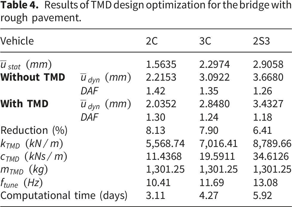
The results in Table 3 indicate successful robust optimization of a TMD. After installation, the DAF fell below the code limit, demonstrating that TMDs can effectively control vibrations from vehicles on rough pavement. Additionally, there was a notable reduction in the bridge’s maximum vertical displacement, with the optimization algorithm successfully lowering it below $Civ$ .

Figure 9 shows the curves with the maximum mean vertical displacements on the bridge’s nodes for each vehicle considered in the analysis.

Figure 9.

Maximum mean displacements in the bridge’s nodes for the static, dynamic without TMD, and dynamic with TMD analyses.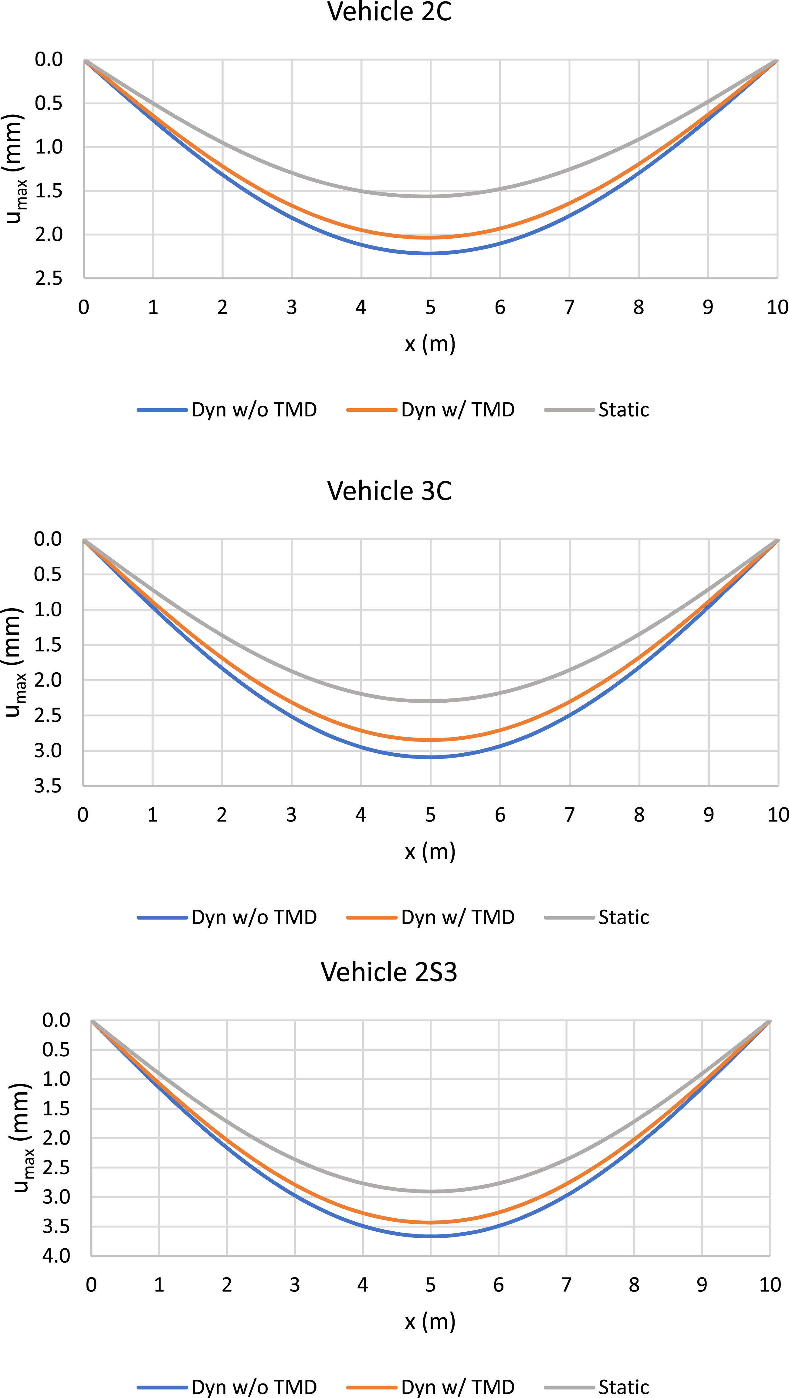

3.5. Design of one TMD for the bridge with a pothole as pavement

This section analyzes the design of a single TMD for a bridge subjected to vehicle passage (2C, 3C, and 2S3) with pothole pavement conditions. The optimization problem, defined by equation (29), was solved using the HBA algorithm with 10 search agents over 25 iterations and 250 random variable samples. The optimization was conducted in parallel running on 8 processors. Results are shown in Table 5.

Table 5.

Results of TMD design optimization for the bridge with a pothole as pavement.

Vehicle		2C	3C	2S3
${\overline{u}}_{stat}\hspace{0.17em}\left(mm\right)$		1.5635	2.2974	2.9058
Without TMD	${\overline{u}}_{dyn}\hspace{0.17em}\left(mm\right)$	3.2459	4.0807	4.3108
	$DAF$	2.08	1.78	1.48
With TMD	${\overline{u}}_{dyn}\hspace{0.17em}\left(mm\right)$	2.7651	3.3388	3.8751
	$DAF$	1.77	1.45	1.33
Reduction (%)		14.81	18.18	10.11
$k_{TMD}\hspace{0.17em}\left(kN/m\right)$		6,002.24	7,140.31	7,592.44
$c_{TMD}\hspace{0.17em}\left(kNs/m\right)$		0.00	15.7125	34.2453
$m_{TMD}\hspace{0.17em}\left(kg\right)$		1,301.25	1,301.25	1,301.25
$f_{tune}\hspace{0.17em}\left(Hz\right)$		10.81	11.79	12.16
Computational time (days)		2.79	4.31	5.24

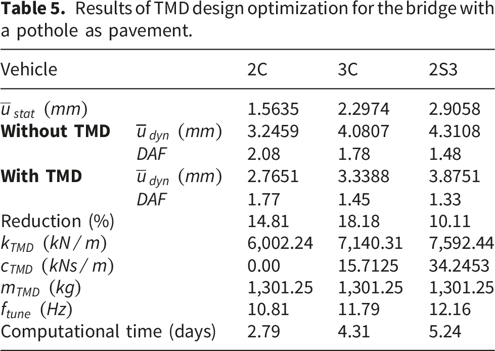
Unlike the results for the TMD design with rough pavement, the optimization algorithm reduced the maximum vertical displacement of the bridge for all vehicles. However, it only achieved a DAF below the $Civ$ limit for vehicle 2S3. For vehicles 2C and 3C, despite a reduction, the DAF stayed slightly above the $Civ$ limit.

The outcome is likely due to the total mass of the vehicles. The 2S3 vehicle’s higher load-carrying capacity produces a high static response and a lower DAF. Additionally, the depth and length of the pothole, treated as a random variable, significantly affect the bridge’s dynamic response, as noted by ²⁵ in their study on pavement irregularities.

Figure 10 shows the graphs with the maximum mean vertical displacements for the bridge nodes for vehicles 2C, 3C, and 2S3.

Figure 10.

Maximum mean displacements in the bridge’s nodes for the static, dynamic without TMD, and dynamic with TMD analyses.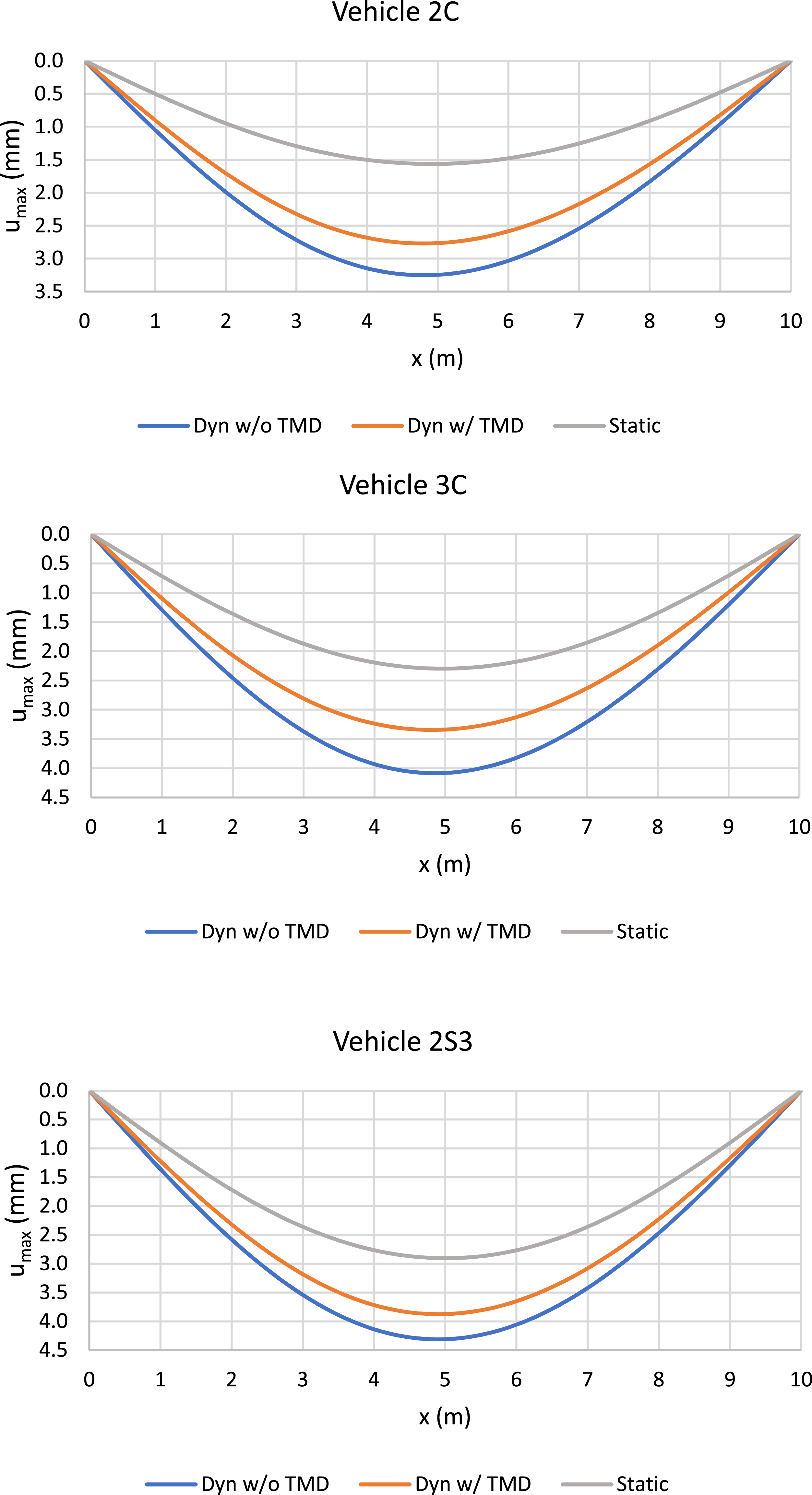

3.6. Design of MTMD for the bridge with a pothole as a pavement

Based on the observations from the results in Sections 3.4 and 3.5, the simulations with a pothole as a pavement condition did not satisfactorily reduce the DAF for two of the three vehicles to at least a value equal to $Civ$ . To improve it, this section focuses on designing and installing three TMDs on the bridge to achieve a better reduction in its dynamic response.

The situation analyzed in the optimization process consists of designing three TMDs with equal parameters tuned to the same frequency. These TMDs were placed at nodes located at 4.6 m, 5 m, and 5.6 m. equation (30) describes the optimization problems solved for the situation considered.

$\begin{array}{ll}Encontar& \overrightarrow{x}=\left[k_{TMD},c_{TMD}\right]\\ Minimize& {\overline{u}}_{\mathit{max}}=E\left[u_{\mathit{max}}\left(\overrightarrow{x}\right)\right]\\ Sujeito\hspace{0.17em}a& 0\le k_{TMD}\le {1.10}^8\hspace{0.17em}N/m\\ & 0\le c_{TMD}\le {1.10}^5\hspace{0.17em}Ns/m\\ & m_{TMD}=0.01M_{st}\hspace{0.17em}kg\end{array}$

(30)

The number of search agents, iterations, and samples used in the HBA algorithm, as well as the code version, are the same as those used in the simulation in Section 3.5. The results obtained from these simulations are presented in Table 6.

Table 6.

Results of the MTMD design.

Vehicle		2C	3C	2S3
${\overline{u}}_{stat}\hspace{0.17em}\left(mm\right)$		1.5635	2.2974	2.9058
Without TMD	${\overline{u}}_{dyn}\hspace{0.17em}\left(mm\right)$	3.2459	4.0807	4.3108
	$DAF$	2.08	1.78	1.48
With TMD	${\overline{u}}_{dyn}\hspace{0.17em}\left(mm\right)$	2.7725	3.3464	3.8806
	$DAF$	1.77	1.46	1.34
Reduction (%)		14.58	17.99	9.98
$k_{TMD}\hspace{0.17em}\left(kN/m\right)$		2,007.35	2,402.12	2,556.35
$c_{TMD}\hspace{0.17em}\left(kNs/m\right)$		0.00	5.2267	11.3279
$m_{TMD}\hspace{0.17em}\left(kg\right)$		433.75	433.75	433.75
$f_{tune}\hspace{0.17em}\left(Hz\right)$		10.83	11.84	12.22
Computational time (days)		3.00	3.59	4.82

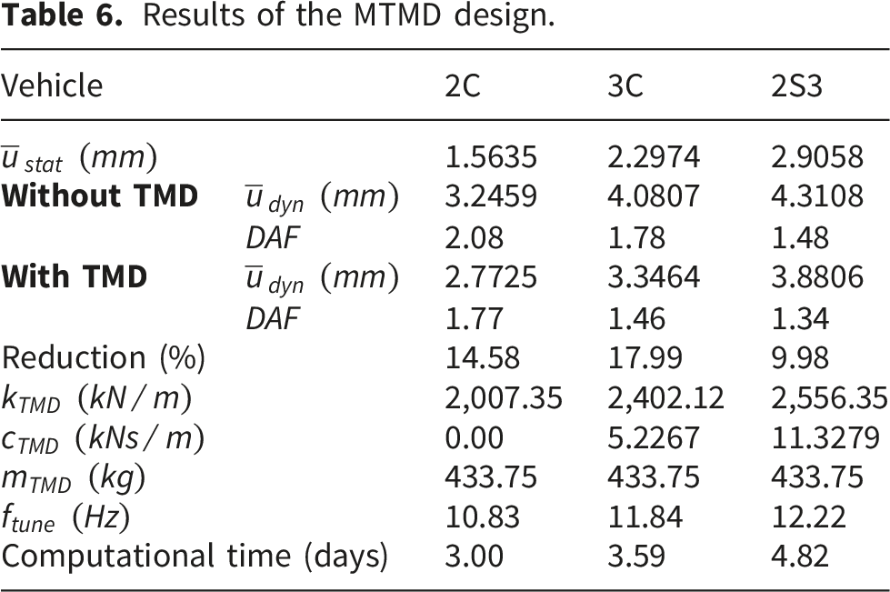
It can be observed that for the situations, the results obtained with the MTMD attached to the structure do not show a significant difference in terms of vertical displacement when compared to the results obtained with only one TMD, with a bigger mass, attached at the center of the bridge.

To improve the reduction of maximum vertical displacement in the bridge, increasing the masses of the TMDs could be considered. However, this could undermine the optimization goals by not providing an economical solution. Given that dynamic responses show little difference between one or three TMDs, the MTMD solution is preferred, as each device is lighter and requires less stiffness and damping to construct.

The high DAF for vehicles 2C and 3C suggests that using only TMDs for vibration control in bridges with a pothole at the entrance may not be ideal. This should be related to the fact that under severe pavement conditions, such as deep potholes, the induced vehicle–bridge interaction forces may contain significant broadband frequency content. In such cases, the structural response may not be governed solely by the first vibration mode. Consequently, while the MTMD remains effective for the dominant modal response, its performance may deteriorate when excitation energy is distributed over a wider frequency range.

This observation brings the possibility of future works to explore other types of devices to reduce the maximum displacement of the bridge caused by the pothole. For example, the use of supplemental viscous dampers can provide broadband energy dissipation that is less sensitive to precise frequency tuning. Additionally, active or semi-active control systems can adapt their response characteristics in real time to varying excitation conditions. Hybrid control strategies, combining the MTMD solution proposed in this research, targeting the dominant mode, with active control mechanisms addressing off-tuned frequency components, also represent a viable solution.

Next, Figure 11 shows the curves with the maximum mean vertical displacement of the bridge’s nodes for the situation analyzed.

Figure 11.

Maximum mean displacements in the bridge’s nodes for the static, dynamic without TMD, and dynamic with MTMD.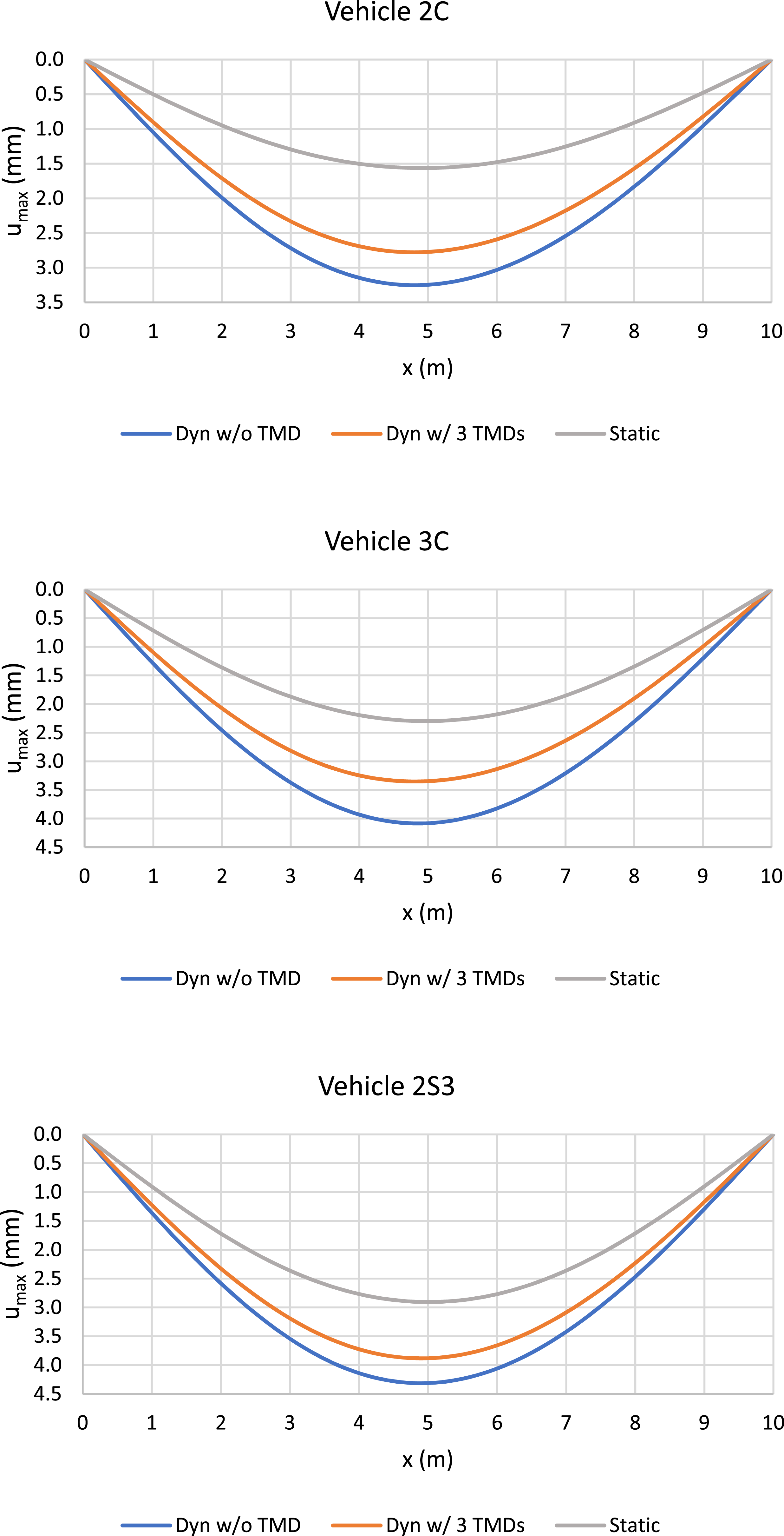

4. Conclusions

This paper aimed to propose a complete and robust methodology not only to conduct dynamic analyses of bridges considering the effects of vehicle-bridge-pavement interaction, including uncertainties in all systems, but also to optimize TMDs; therefore, based on the results obtained, it is concluded that this main objective was successfully achieved.

The results of the robust optimization of the TMD obtained by the proposed methodology using the HBA showed that the mean maximum vertical displacement at the center of the bridge was reduced in all situations evaluated, that is, for the three types of vehicles and for the two types of pavements, proving the success of the proposed methodology.

Upon closer examination of the results obtained, it was possible to note that the mean maximum displacement of the bridge was reduced by more than 7.5% and 14.4% for situations with uneven pavement and obstacles, respectively.

The tests carried out with multiple TMDs showed that the results obtained for each of the vehicles were not very different from the results obtained for just 1 TMD, that is, the proposed methodology also proved to be effective for optimizing multiple TMDs.

Regarding the code parallelization presented for evaluating the objective function used to design the TMD parameters, it is noteworthy that the optimization process for evaluating TMD parameters took an average of 4.12 days, with the 2S3 vehicle requiring the longest time at 5.33 days. The computational time would likely double in a fully sequential version. Parallelization makes this robust optimization process feasible.

Therefore, the robust optimization methodology proposed in this paper, combined with parallel processing, can be a useful tool to assist designers with the project of new structures or propose a solution to extend the service life of the existing ones.