
Abstract
In this paper, we investigate the solution of fractional differential equations (FDEs) based on the reproducing kernel method. A reproducing kernel space is constructed using Legendre polynomials. Within this space, the ɛ-approximate method is applied to analyze the condition number of the matrix, and the stability and convergence of the proposed algorithm are examined. Finally, three numerical examples are presented to verify the effectiveness of the method. The obtained absolute errors are smaller than those reported in the reference literatures. This work provides an accurate and reliable numerical tool for solving FDEs.
Keywords
Introduction
In recent years, there has been increasing focus on the study of fractional differential equations (FDEs). The primary reason for this is that fractional calculus operators can describe many engineering problems more accurately than traditional integer-order calculus operators.1–3 FDEs have attracted significant attention from various scientific fields, including physics, earthquake dynamics, signal processing, fluid mechanics, 4 chaotic dynamics, biology, 5 electromagnetic waves, polymer science, thermodynamics, and so on. 6 FDEs are often characterized by weakly singular kernels and are more complex than integer-order differential equations. In many cases, it is difficult to obtain analytical solutions, prompting researchers to focus on approximate solutions and develop a variety of methods, 7 such as the finite difference method, 8 the local meshless method based on Laplace transforms, 9 the Laplace transform method, 10 variational iteration methods, 11 spectral methods,12,13 and the shooting method, 14 etc. An efficient method for solving a class of higher-order fractional differential equations with general boundary conditions is proposed by introducing appropriate basis functions. 15 Additionally, a small-parameter asymptotic method for solving fractional differential equations is proposed: by decomposing the field variable and the Riemann–Liouville integral, this method converts time-fractional differential equations into a system of two coupled integer-order partial differential equations, and solving the latter yields the solution to the original fractional differential equation. 16 To the best of our knowledge, the reproducing kernel space is widely recognized as an ideal framework for numerical analysis research. In previous work, the Taylors formula or Delta function was used to construct the reproducing kernel space,17–20 which has been proved to be an effective tool to solving various kinds of differential equations.21,22 Building on this foundation, the application scope of the reproducing kernel method has been further extended to solve fractional differential equations with periodic conditions in Hilbert space. 23
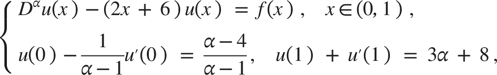
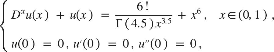
In this paper, we mainly focus on the numerical solution of FDEs as follows

The remaining part of this paper is organized as follows: In the Preliminaries section, the construction of a basis for the reproducing kernel space using Legendre polynomials is presented. An efficient technique based on the ε-approximate method for solving (1.1) is then introduced, accompanied by a theoretical analysis of the uniqueness, stability, and convergence of the approximate solution for homogeneous equations. Finally, Numerical results are presented to demonstrate the validity of the proposed method.
Preliminaries
Caputo operator theory
The Caputo fractional order derivative is defined by
13
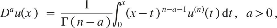
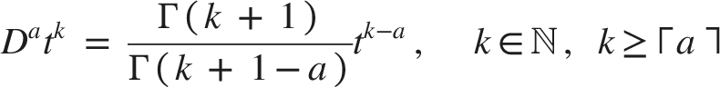
The following properties are satisfied by the operator D
a
for n − 1 ≤ a < n
Basis of reproducing kernel space based on Legendre polynomials
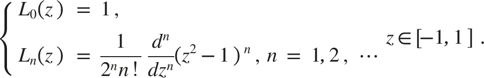
The well-known Legendre polynomials are defined on the interval [−1, 1] and its recurrence formula
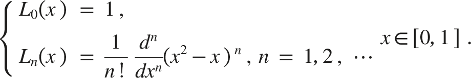
Let z = 2x − 1, we can get the following formulation in the interval [0, 1]
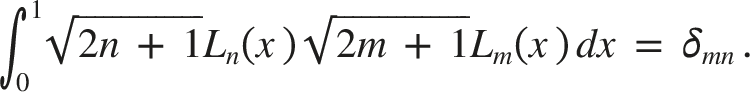
The Legendre polynomials has following properties
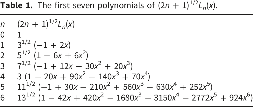
The first seven polynomials of (2n + 1)1/2L n (x).
Let

the inner product 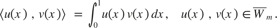
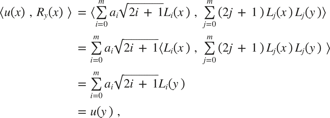
Then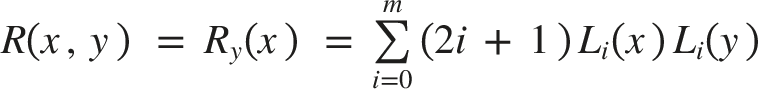
Proof. Using,
28
we can prove that
Let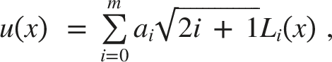
Using
29
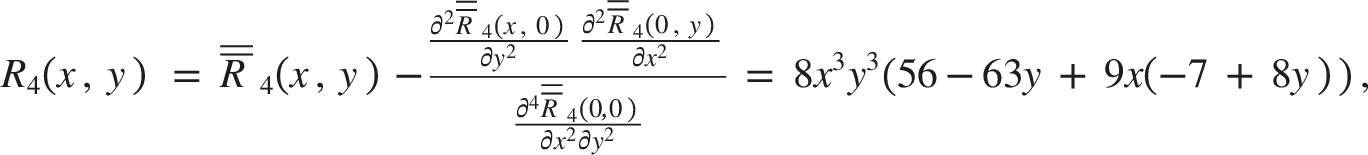
and the reproducing kernel of • Space • Space • Space


An efficient technique based on ɛ-approximate method for equation
Theoretical analysis of the algorithm for equation
Let

According to (3.1), a linear operator 
It has the following properties.
The operator
Proof. Obviously, 
Let v(x) ∈ W
m
[0, 1], by the reproducibility property of the reproducing kernel function R
m
(x, y) ∈ W
m
, there exist positive constants S
i
(i = 0, 1, 2, ⋯ ), such that
By employing the aforementioned formula and utilizing Cauchy–Schwarzs inequality, a direct calculation can be performed to ascertain the existence of positive constants C and S, such that
Then
Similarly, we have
Applying (3.3), (3.4), and (3.5), one gets
Let 
For ∀ɛ > 0, if
According to (1.4), when k = m − 1 (m = 2, 3, ⋯ ), there is 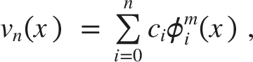

The ɛ-approximate method for equation (3.1) is as follows: seeking 
The coefficients 


The numerical scheme (3.7) has a unique solution provided that
Proof. It is sufficient to prove the linear system AX = 0 has only zero solution. Assume that
Multiplying both sides of (3.9) by x
j
and a cumulative summation yields that
Stability and convergence analysis
We will first discuss the stability of our proposed method. The condition number of matrix A is defined as follows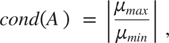
The eigenvalue of A obtained by (3.8) is bounded by
Proof. Let μ is an eigenvalue of 
Summing x
i
from 0 to n in above formula, we derive that
If
For v ∈ W
m
, if
Proof. Let 
The numerical scheme for getting the ɛ-approximate solution of (3.7) is stable.
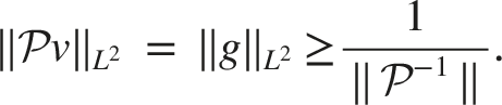
Proof. Denote μ be the eigenvalue of A obtained by (3.7), then we have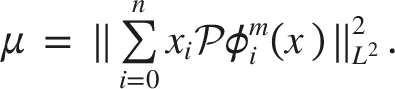
Combining the fact that 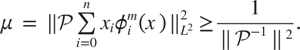
So, the condition number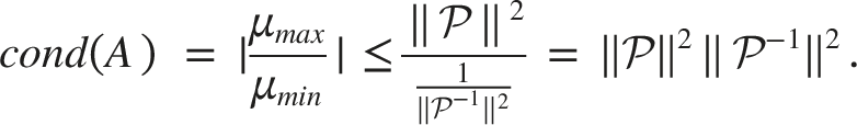
It means that the condition number is bounded, so our algorithm is stable. 31 □
Next, we will provide the convergence analysis of the presented scheme.
Let v ∈ W
m
[0, 1] be the exact solution of (3.1), then approximate solution v
n
∈ W
m
[0, 1] converges to v uniformly.
Proof. Note that

It means v n converges to v uniformly on interval [0,1]. □
Similarly, we can proof each order derivative
Numerical results
In this section, three numerical examples are presented to demonstrate the effectiveness of the proposed algorithm.
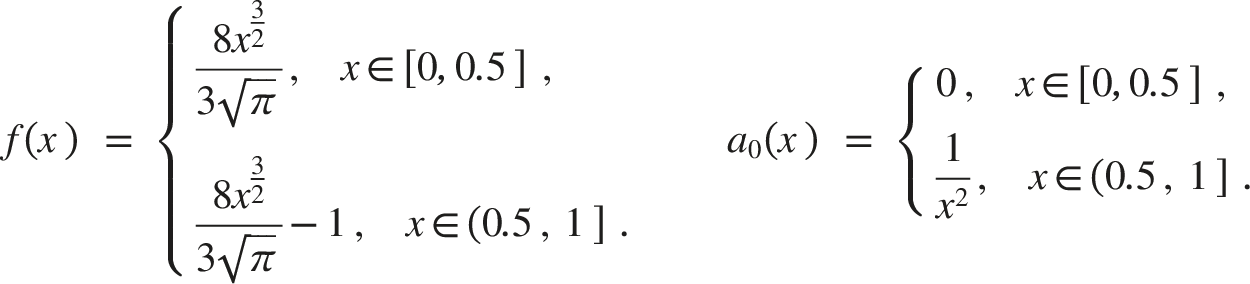
When α = 0.5

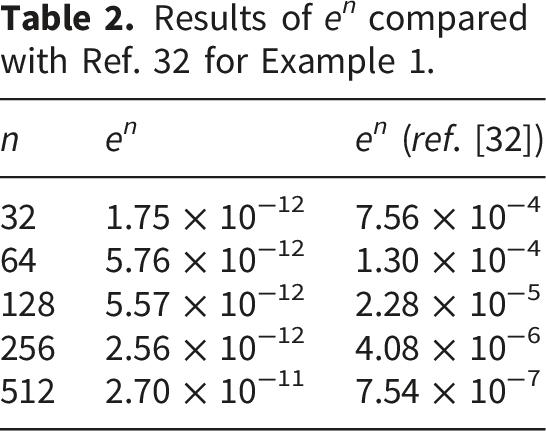
Results of e n compared with Ref. 32 for Example 1.
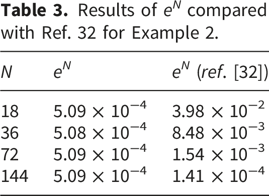
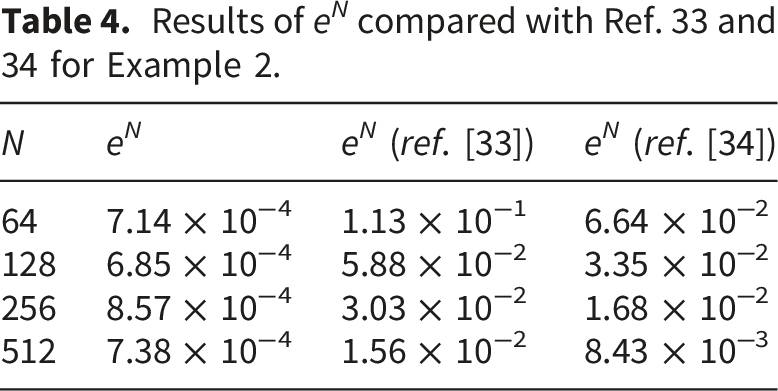
Consider the example 2 in Ref. 32 with α = 1.9
Results of e N compared with Ref. 32 for Example 2.
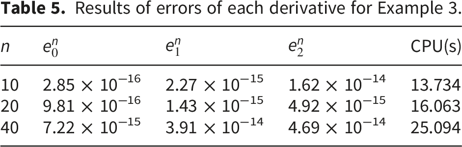
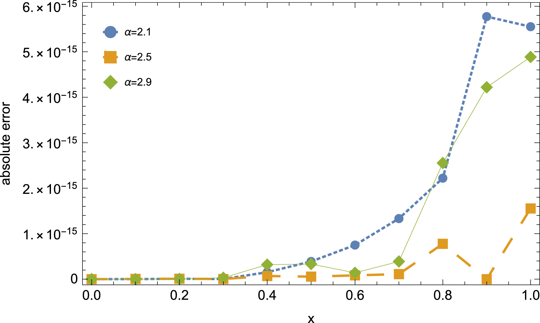
Consider the following example with 2 ≤ α ≤ 3,
Results of errors of each derivative for Example 3.
Figures 1 and 2 show that the absolute-errors corresponds to different the number of basis n and different values of fractional parameter α. The Absolute-errors with α = 2.3 for different the number of basis n. The Absolute-errors with n = 10 for different values of fractional parameter α.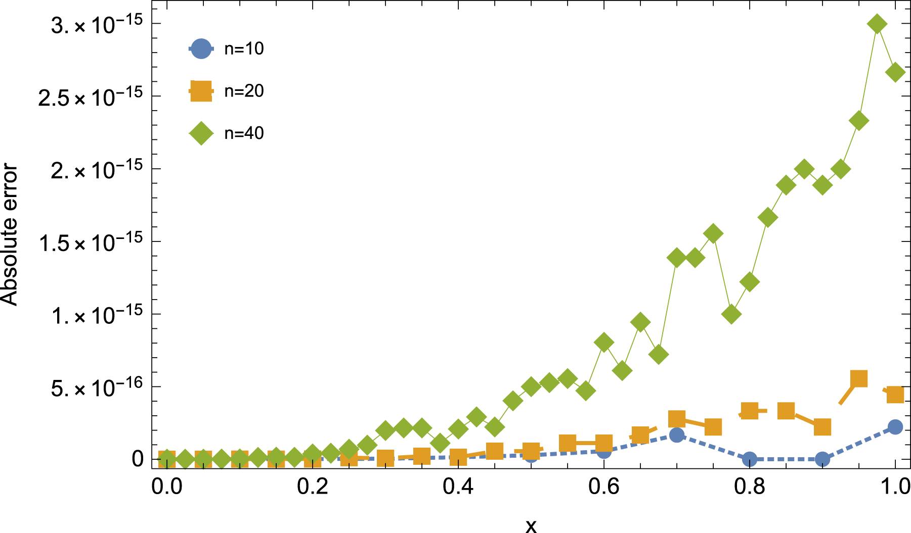
Conclusion
This paper proposes an efficient numerical scheme for solving FDEs by integrating the reproducing kernel space theory with the ɛ-approximate method. The method proposed in this paper has the following advantages. First, in the absence of an exact solution, the approximate solution obtained by this method exhibits good agreement with the theoretical exact solution. Both the approximate solution and its derivatives converge uniformly to the exact solution. The numerical examples further verify the effectiveness and superiority of the proposed method. Second, the results demonstrate that the errors of the scheme are smaller than those reported in the reference literature. Furthermore, the computational time of this method is relatively short. Third, this method boasts strong applicability in physics, including transonic multiphase flows and the electric circuit model of fractional stiff differential equations.35,36 Moreover, it is extensible to solving fractional integro-differential equations, stochastic fractional differential equations and high-dimensional systems.
Footnotes
Acknowledgment
We would like to thank the reviewers for their valuable comments, which have significantly improved the quality of this paper.
Funding
The authors disclosed receipt of the following financial support for the research, authorship, and/or publication of this article: This work was supported by The Science and Technology Development Fund of Tianjin Education Commission for Higher Education (2024kJ124).
Declaration of conflicting interests
The authors declared no potential conflicts of interest with respect to the research, authorship, and/or publication of this article.