Sage Journals: Discover world-class research

Abstract

Structural health monitoring (SHM) is of critical importance in a variety of fields. Oftentimes the studied system also possesses complex behavior, turning the assessment of such structure difficult. One of the solutions for high complexity systems is the use of data-driven approaches, such as machine learning and deep learning techniques. However, training traditional deep learning architectures can require large amounts of data, which may not be available for both health and damaged conditions in operating structures. This study proposes the adaptation of GoogleNet allied with transfer learning for damage detection in vibrational structures. By converting vibrational signals into scalograms, using the Continuous Wavelet Transform (CWT) both the time and frequency information of the measurement can be kept and the Convolutional Neural Network (CNN) can classify the time-series dataset into different damage scenarios. This methodology initially employs full-field measurements from the structure, allowing fine-tuning of the GoogleNet, which also requires less amount of data. Later, traditional accelerometer measurements are employed for testing and classification of different damages. This approach poses good accuracy for anomaly detection, using diverse frequency excitation as input, demonstrating a great capability to perform image processing with vibration signal analysis, allowing local testing for damage detection and real-time signal classification.

Keywords

vibration signal classification transfer learning scalograms convolutional neural networks anomaly detection

Introduction

Structural Health Monitoring (SHM) of systems can provide accurate information on the working conditions and prevent possible failures in different industrial systems. Detecting early warning signals indicating imminent failure avoids problems from aggravating. It is a research field with a variety of different applications, for example, civil infrastructure,^1,2 wind turbine blades.³ How the data is collected for monitoring is another focus of study, using traditional sensing techniques to noncontact technologies.^4,5 To overcome such challenges, SHM can be performed using a model-based approach. Where some previous information is known, for example, using a digital twin^6,7. However, due to the complexity of the system behavior, data-driven approaches are often employed in SHM.^8,9 For instance, using strategies based on a hybrid Dynamic Bayesian network,¹⁰ using signal processing techniques¹¹ or a probabilistic principal component analysis-based.¹² Nonetheless, in the recent literature, most of the efforts relies on artificial intelligence models for enhancing pattern identification.¹³

Among the different architectures available for deep learning, convolutional neural networks are commonly used for anomaly detection.^2,14,15 In addition, considering the gradual change of the system’s condition, Recurrent Neural Networks (RNNs) and Long Short-Term Memory (LSTM) networks are also employed in SHM.¹⁶

Among such methods, ultrasonic testing uses vibration signals which are useful for detecting flaws on the surface.¹⁷ Lower frequencies can be used depending on the target.¹⁸ There are different systems for recording vibration signals although vibrometers and accelerometers are commonly used. Some studies use vibrational analysis where there are several methods such as vibrational signal classification.¹⁹ A common strategy for signal classification is time-frequency analysis by transforming the signal from the time domain into the frequency domain by using the Fast Fourier Transform (FFT) and then creating a spectrogram.²⁰ FFT is not able to incorporate multiple scales, however, wavelet transformation does lead towards optimal time-frequency resolution.²¹ The time-frequency diagrams obtained show the combined information in the time domain and frequency domain, which directly reflect the change of the frequency components of the signals over time.

A spectrogram is a time-frequency representation of the signal and offers a fixed time and frequency resolution. They have succeeded in practical applications in the fields of in-process monitoring, music, sonar, radar, and speech processing, supplying image color information very suitable for image recognition.^22–24 A scalogram is a time-frequency representation of the signal by wavelet transformation. This representation offers the brightness or the color which is useful to indicate coefficient values at corresponding time-frequency locations.²⁵ However, while a spectrogram focuses on representing how frequencies change over time, a scalogram focuses on showing how the energy of the signal varies with scale (or frequency) and time. This method plays an important role in various engineering and structural analysis contexts, and it is instrumental in identifying structural anomalies, defects, or irregularities.^26–28

Within this context, artificial intelligence has helped particularly with conventional machine learning methods, deep learning methods and transfer learning (TL) methods. Machine learning has shown promising results in various areas of engineering.²⁹

Deep learning methods assume that training and test data fall by the same distribution. Interestingly, TL methods do not necessarily make such an assumption.²⁵ Besides, TL methods improve performance for classification systems respect with conventional machine learning methods.³⁰

Nonetheless, equipment for testing is expensive and processing record data is a time-consuming task. With this regard, the authors suggest a novel approach to perform the Non-destructive Test (NDT) field by using Deep Transfer Learning (DTL). Transfer learning (TL) is a branch of machine learning (ML) that aims to leverage common knowledge from related but different application scenarios to enhance the performance of artificial intelligence (AI) algorithms in specific tasks. Conventional machine learning methods require data collection, feature extraction and classification which are a laborlabor-intensive and time-consuming task. On the other hand, deep learning methods assume that training and test data follow the same distribution. However, in practical scenarios, working conditions often vary significantly between different tasks. Consequently, the distribution of test data gathered from these diverse conditions differs from that of the training data. Moreover, if the test data originate from different equipment, the fault diagnosis accuracy of deep learning models may substantially decrease, even when the fault types remain consistent.^25,30,31

Fortunately, TL methods do not necessarily make such an assumption. Besides, some authors show how TL methods improve performance for classification systems.^30,32–34 They have shown promise in overcoming limitations such as sparse training data and poor generalization. DTL combines the advantages of deep learning in feature representation with the benefits of transfer learning in knowledge transfer. DTL is increasingly being utilized, particularly in practical applications within the manufacturing industry, as it can effectively learn hidden transferable knowledge and capture complex patterns. This integration with deep learning models enhances reliability, robustness, and accessibility of deep-learning-based methods, making them more suitable for industrial applications, such as intelligent fault diagnosis in industrial engineering.³⁵

In this article, the authors employ a dedicated convolutional neural network for image classification to identify anomalies in vibrational signals. These signals are obtained from both a laser vibrometer and accelerometers, capturing the amplitude of oscillations of a metallic plate in each case. The dataset was collected over multiple days in a controlled indoor laboratory environment at room temperature, with slight variations between acquisition sessions. The test specimen used was a metallic plate designed for experimental validation, serving as a first step toward applying this methodology to real working systems. The next sections of this work are divided as a methodology section which will be explained the details on the neural network implemented, as well as the signal processing techniques used for data processing. Later the experimental setup will be presented, with the results for each case study. Finally, a conclusion will be provided.

Methodology

This section presents the preprocessing techniques used to obtain the dataset for training and testing the modified GoogleNet. In addition, an explanation of the original structure of the neural network and the modifications needed to work with the specific dataset and the hyperparameters selected for the study are provided. The framework of the proposed approach is provided in Figure 1.

Figure 1.

Framework for the DTL method.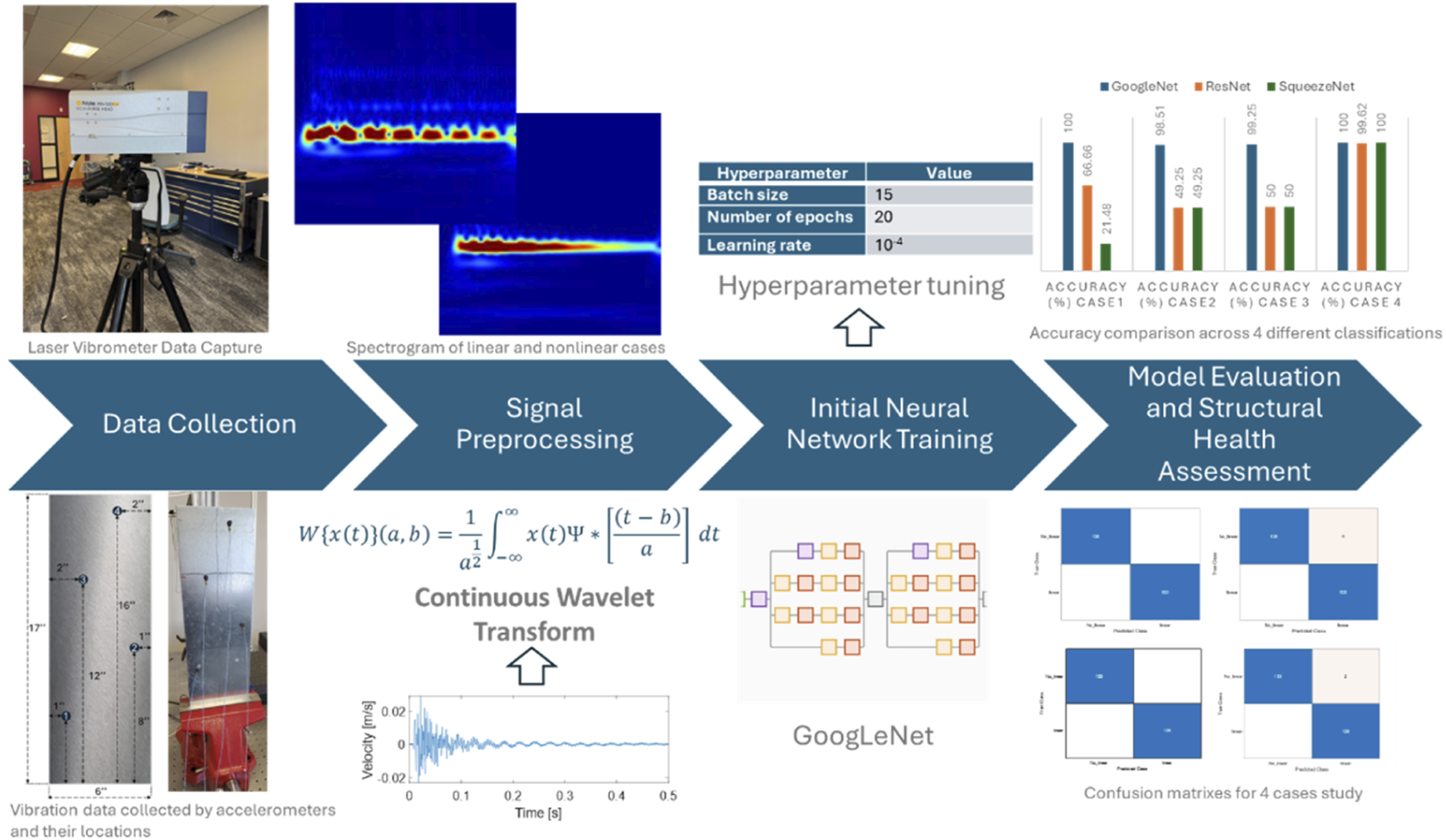

The overview of the proposed approach consists of obtaining full-field information about the system. In this application, a Laser Doppler Vibrometer was employed. The measurement obtained for each of the points will then be converted to scalograms to keep both temporal and frequency information. The dataset will then be used to train GoogleNet. In parallel, data will be collected by using traditional sensing techniques, such as accelerometers. Those measurements will be sparse and contain limited information about the system. The same wavelet transformation will be applied to the new dataset, allowing the fine-tuning of the network. Finally, the model will be evaluated based on separate data that was not used during training.

The next subsections will present the processing technique in more detail, as well as detailed information regarding GoogleNet and the transfer learning procedure.

Preparation and creating time-frequency representations

Initially, the vibration measurements are normalized and converted into scalograms using the Continuous Wavelet Transform (CWT). The scalograms represent the absolute values of the CWT coefficients of each signal, enabling the extraction of valuable time-frequency features. This transformation converts time-series data into a visual format that highlights the evolution of frequency components over time, creating an image-like representation.

To ensure a stable and consistent transformation, the CWT was performed using a filter bank with a sampling frequency of 50 kHz and Voices Per Octave set to 12, providing a balance between time and frequency resolution. The CWT is defined in equation (1).

W {x (t)} (a, b) = \frac{1}{a^{\frac{1}{2}}} \int_{- \infty}^{\infty} x (t) Ψ^{*} [\frac{(t - b)}{a}] d t

(1)

The wavelet transform is calculated by convoluting the input signal with a wavelet function, based on equation (1), $x (t)$ is the time domain signal and $Ψ$ is the wavelet function. For this case, the function used was Morse wavelet due to its adaptability in signal analysis. It is described in its generalized form in equation (2).

Ψ_{P, γ} (ω) = U (ω) C_{P, γ} ω^{\frac{P^{2}}{γ}} e^{- ω^{γ}}

(2)

where

U (ω)

is the unit step function in the frequency domain,

C_{P, γ}

a normalization constant.

P^{2}

is the time-bandwidth product, and

γ

characterizes the symmetry of the wavelet function. For this application, the value for both constants is 3, which optimizes the trade-off between time localization and frequency resolution. These settings allow the model to capture fine details in the vibration signals while maintaining computational efficiency for deep learning classification.

As the output of the CWT is a two-dimensional matrix with time and frequency information, each matrix can be converted to a RGB image which then will be used as the input for the neural network, enabling the model to learn from the complex patterns and features inherent in the structural vibrations. Figure 2 shows the differences between the linear and nonlinear cases.

Figure 2.

Spectrogram of linear and nonlinear cases. (a) Linear and (b) nonlinear.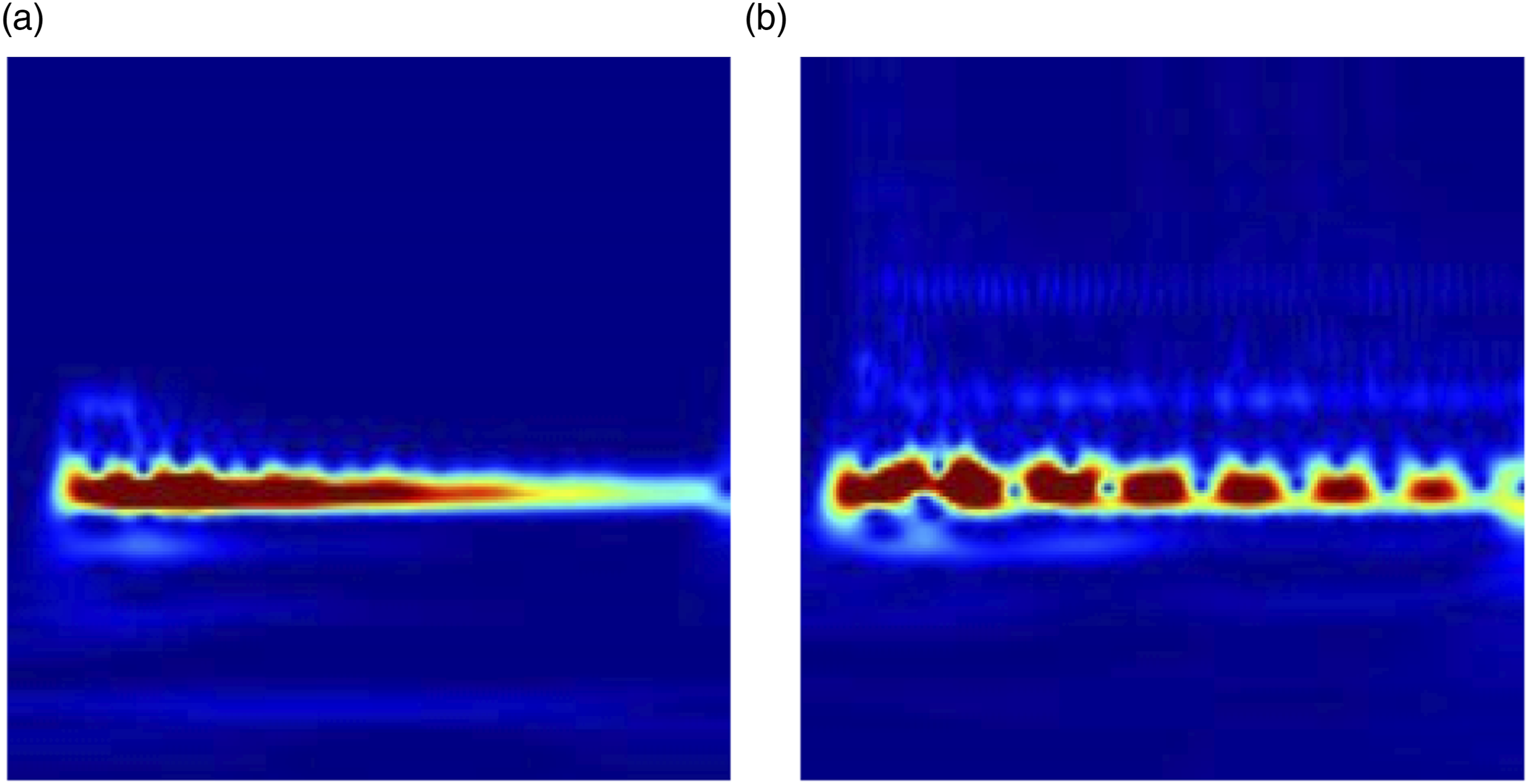

The use of CWT and the resultant scalograms are instrumental in addressing the complex nature of vibration signal analysis. CWT is particularly adept at revealing aspects of data that other time-frequency methods, such as the Short-Time Fourier Transform (STFT), might miss. Unlike STFT, which has a fixed resolution across all frequencies, CWT provides a variable resolution that offers finer temporal resolution at higher frequencies and finer frequency resolution at lower frequencies. This adaptive resolution is crucial for detecting subtle anomalies in vibration patterns that may indicate structural faults or changes.

Transfer learning strategy

Considering the complexity of vibrational data for classification, as well as the limitations on data acquisition for operational systems, a transfer learning approach was adopted, repurposing a well-known pre-trained CNN architecture: GoogLeNet, also known as Inception v1.³⁶ Its architecture includes several key components: convolutional layers, pooling layers, inception modules, fully connected layers, and a SoftMax layer. The convolutional layers are responsible for extracting features from input images, while the pooling layers reduce the dimensionality of these features, retaining essential information and reducing computational cost. Inception modules apply parallel convolutions with different filter sizes and concatenate the results, capturing features at multiple scales. The fully connected layers perform the final classification based on the extracted features, and the SoftMax layer converts the outputs into probabilities for each of the classes. This network, originally designed to classify 1000 different categories of images, is adapted to the domain of vibration signal analysis and damage classification using the time-frequency representation obtained by the CWT.

To evaluate the most suitable architecture for vibration signal classification, three convolutional neural networks were considered: GoogLeNet, ResNet, and SqueezeNet. These models were selected for their balance between representational power and computational efficiency. Among them, GoogLeNet was chosen for the main analysis due to its superior performance in preliminary evaluations, as will be detailed in the results section.

To effectively apply transfer learning, GoogLeNet was adapted by freezing its convolutional and inception layers, which retain the pre-trained ImageNet weights that capture general image features. These layers were not modified, as they efficiently extract multi-scale spatial patterns from the scalograms. Only the final classification layers were retrained to specialize in vibration signal classification.

To enhance learning in the new layers, the fully connected and classification layers were replaced. The original “loss3-classifier” layer was substituted with a new fully connected layer, where the number of output neurons was adjusted to match the number of vibration signal classes in the dataset. The final classification layer was also replaced with a new one that directly maps the extracted features to the new class labels. These modifications ensure that the model learns the specific damage classification task while leveraging the general feature extraction capability of the frozen layers.

To mitigate overfitting, a dropout layer with a probability of 0.6 was introduced before the final classification step. This technique prevents the model from relying too heavily on specific neurons, promoting better generalization. The dropout rate was selected after evaluating several values between 0.3 and 0.7, aiming to balance model regularization and classification performance. Several configurations were tested, varying the number of unfrozen layers and the dropout rate. The selected setup demonstrated the best trade-off between accuracy and stability, allowing effective feature extraction while preventing over-adaptation to the training data.

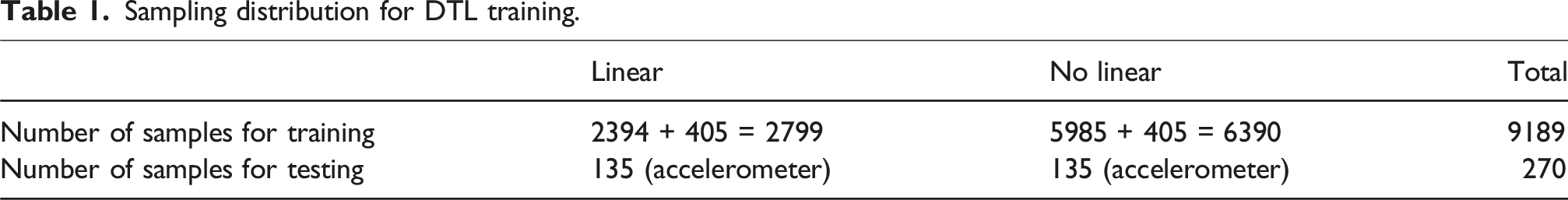
The dataset used for training included full-field vibration measurements, while testing was conducted using accelerometer data collected from specific locations on the structure. This approach evaluates the model’s ability to generalize from full-field vibration data to sparse sensor-based measurements. The number of samples for each dataset partition is summarized in Table 1.

Table 1.

Sampling distribution for DTL training.

	Linear	No linear	Total
Number of samples for training	2394 + 405 = 2799	5985 + 405 = 6390	9189
Number of samples for testing	135 (accelerometer)	135 (accelerometer)	270

Finally, the hyperparameters used for training the neural network are presented in Table 2.

Table 2.

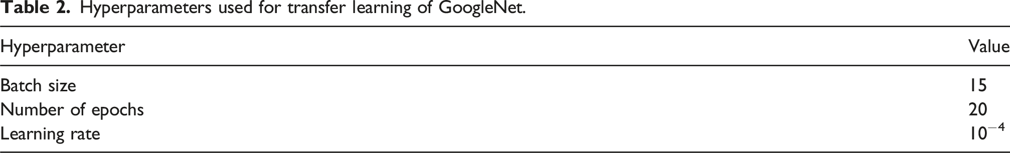
Hyperparameters used for transfer learning of GoogleNet.

Hyperparameter	Value
Batch size	15
Number of epochs	20
Learning rate	10⁻⁴

For transfer learning, maintain the features of the first layers of the pre-trained network (the weights of the transferred layers). To delay the learning in the transferred layers, the initial learning rate was set to a small value of $10^{- 4}$ , a common choice in transfer learning scenarios. In the previous step, the learning rate factors of the fully connected layer were increased to accelerate learning in the newly added final layers. This combination of learning rate adjustments results in fast adaptation where needed while preserving the pre-trained knowledge in earlier layers. Then, the network is retrained to fine-tune the classification task for vibration-based damage detection.

Training the vibration signal classifier

The process of training a neural network involves iteratively minimizing a loss function.

In this case Cross-Entropy loss function is used for measuring the performance of the classification model. Cross-Entropy loss increases as the predicted probability diverges from the actual label.

L = - \frac{1}{2 N} \sum_{i = 1}^{N} [y_{i} \log (p_{i}) + (1 - y_{i}) \log (1 - p_{i})]

(3)

where:

• $N$ is the number of samples.

• $y_{i}$ is the true label for the $i^{t h}$ sample (0 or 1)

• $p_{i}$ is the predicted probability of the $i^{t h}$ sample.

This minimization is accomplished through a gradient descent algorithm. Having used sigmoid activation function for the cross-entropy loss function, the gradient with respect to the weights in the output layer is as follows:

\frac{\partial L}{\partial w_{i j}} = \frac{1}{N} \sum_{i = 1}^{N} (p_{i} - y_{i}) \frac{\partial p_{i}}{\partial w_{i j}}

(4)

where

\frac{\partial p_{i}}{\partial w_{i j}}

is the derivative of the estimated output with respect to each of the weights

w_{i j}

. The gradient descent for the neural network is computed based on a chain derivation between each layer and activation function and the estimated output. Combining these, the gradient descent update rule for the weights in the output layer when using binary cross-entropy loss with sigmoid activation is as follows:

w_{i j}^{(t + 1)} = w_{i j}^{(t)} - η \frac{\partial L}{\partial w_{i j}}

(5)

where

w_{i j}^{(t)}

are the weights on iteration

t

and

η

is the learning rate. In each iteration, the gradient of the loss function is evaluated, and the algorithm updates the weights of the network.

The learning rate is a crucial hyperparameter in this setup, initially set to a lower value to prevent overshooting during the early phases of training. This rate is gradually increased to allow for quicker convergence once the network starts learning the basic patterns.

The training process involves feeding the network with mini batches of data, which helps in stabilizing the learning and reduces the computational cost. Typically, each batch contains a mix of different types of vibration scenarios to ensure the model learns to generalize across various conditions. The training continues for a predefined number of epochs, which is determined based on the balance between training accuracy and validation performance to avoid overfitting.

Validation is an integral aspect of training, helping to assess the network’s performance and generalization capabilities. In the absence of a sufficiently large dataset for separate training, validation, and testing sets, the validation accuracy is treated as a measure of the network’s overall accuracy.

In our case, we have utilized a complete dataset from vibrometers. For each of the following cases, we added a subset (3 accelerometers) of data from vibrometers to train and validate the neural network, reserving the data from one accelerometer for the testing phase. This approach allows us to verify whether the network generalizes effectively or exhibits any form of overfitting.

Case studies

The dataset used in this study is designed to evaluate the capabilities of the deep learning model in differentiating between linear and nonlinear vibration behaviors in a metallic structure under varied experimental conditions. This comprehensive analysis is structured around two distinct scenarios that simulate real-world structural challenges.

Scenario 1: Linear vibration analysis

In the first scenario, vibration signals are collected from a cantilever aluminum plate, with 6 inches of width, 17 inches height and 0.05 inches thickness. A mechanical shaker is attached to this structure to induce vibrations across a spectrum of frequencies. A Laser Doppler Vibrometer (LDV) measures these vibrations, capturing data at 133 mesh points of the surface of the structure. Each point undergoes an average of ten measurements to enhance the reliability and clarity of the data by improving the signal-to-noise ratio. This comprehensive mapping generates 133 distinct signals, which collectively depict the vibration propagation throughout the structure under uniform conditions without any introduced defects or irregularities, hence termed as the “linear” scenario.

Scenario 2: Introducing nonlinearities with bumpers

Contrasting with the first case, the second scenario introduces an additional layer of complexity through the placement of non-attached rubber bumpers. These bumpers are not fixed to the structure but are positioned close enough to impact the vibration patterns during the operational simulation. Their presence introduces dynamic nonlinearities as they intermittently and randomly contact the structure during vibrations. This interaction creates variable and complex vibration behavior that significantly differs from the linear scenario. The placement of these bumpers at various points aims to enrich the dataset, simulate different damage conditions and test the ability of the model to generalize from complex, nonlinear input data.

Bumpers have been introduced into the signal sets in a specific manner to capture various signal characteristics for analysis. Here’s how they are organized:

• Nonlinear Set 1: This set is composed exclusively of signals collected with Bumper 1 installed. This allows for the analysis of the impact of Bumper 1 on signal properties without interference from other variables.

• Nonlinear Set 2: Similarly, this set consists solely of signals gathered with Bumper 2 in place. This setup isolates the effects of Bumper 2 on the signals.

• Nonlinear Set 3: This set is an exception as it comprises signals collected with both Bumpers 1 and 2 simultaneously. This dual-bumper setup is used to study the combined effects of Bumpers 1 and 2 on signal characteristics.

• Nonlinear Set 4: This set includes signals that are exclusively collected with Bumper 3, allowing for focused analysis on the changes induced by Bumper 3 alone.

• Nonlinear Set 5: Comprised solely of signals with Bumper 4.

• Nonlinear Set 6: This final set includes signals that are exclusively collected with Bumper 5.

Each set enables the analysis of specific bumper effects in isolation or in combination, aiding in a detailed understanding of their impacts on signal behavior as shown in Figure 3.

Figure 3.

Location of different bumpers on the plate to generate abnormal vibrations.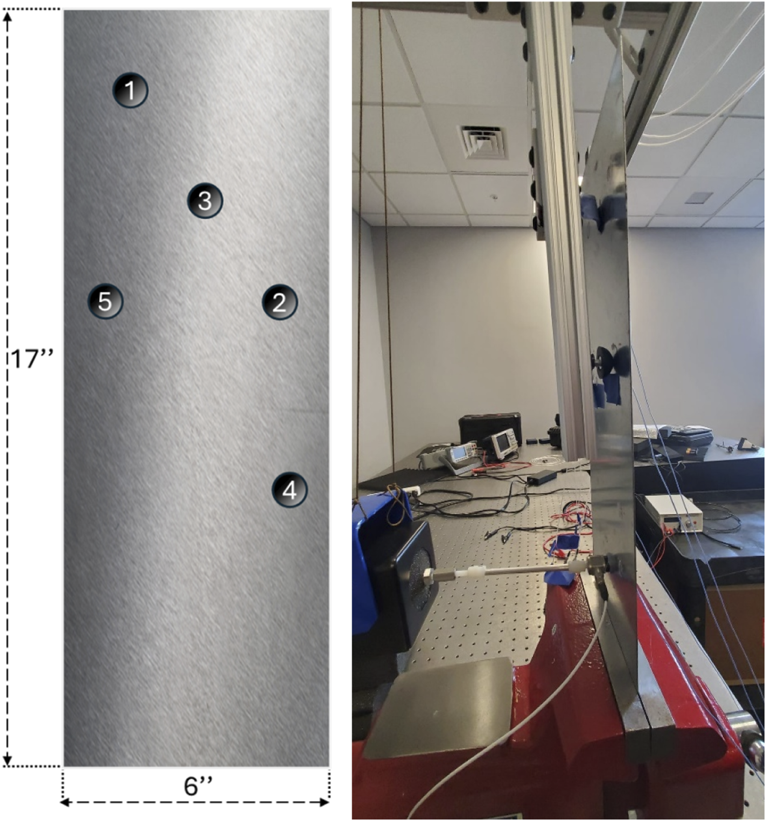

Frequency selection and experimental design

Initially, a modal test was performed into the linear plate, to find its natural frequencies and mode shapes. Using those natural frequencies, nine frequencies were selected from low to high frequency as excitation and those responses were used as input for GoogleNet to classify damage. Figure 3 shows the FRF plot for the plate in blue and the selected frequencies as dashed lines in black (Figure 4).

Figure 4.

FRF of linear plate and selected narrowband frequencies.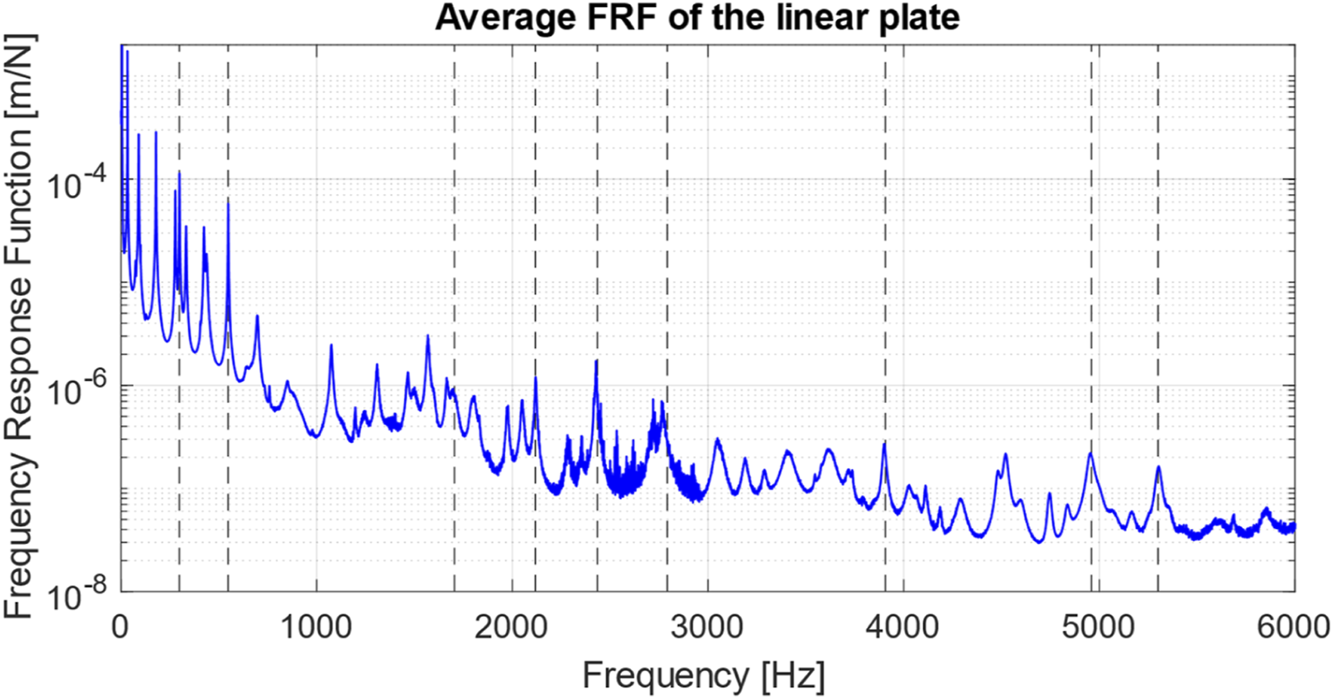

The selection of excitations focused on frequencies that demonstrated heightened energy or amplitude, indicative of significant vibrational activity. These included 298 Hz, 548 Hz, 1704 Hz, 2118 Hz, 2435 Hz, 2792 Hz, 3907 Hz, 4960 Hz, and 5300 Hz, ensuring a robust set that could challenge the model across a broad operational spectrum. To observe the influence of bumper placement on the vibration of the plate, a specific method is utilized.

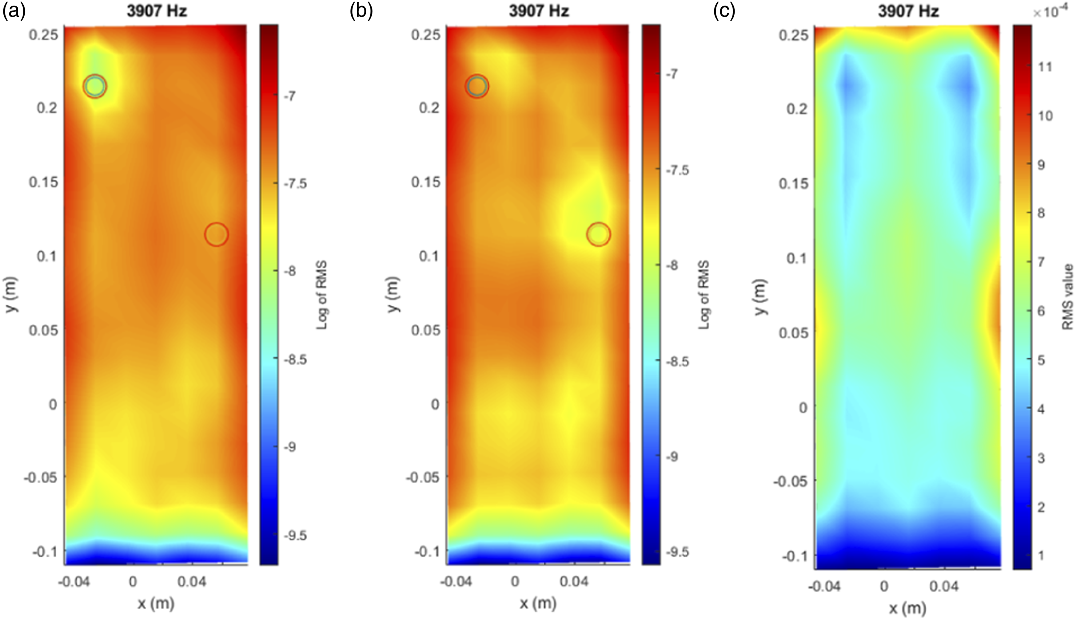
Before introducing the neural network for damage classification, an initial exploratory analysis was performed to verify whether the vibration signals contained detectable changes associated with the presence of bumpers. Following the methodology proposed by Moll et al. and Pawel et al.,^37–39 the RMS value of each signal was computed and logarithmically scaled to enhance local anomalies. This technique worked effectively when using the full-field mesh obtained from the laser vibrometer, revealing how the bumpers influenced vibration intensity in specific regions of the plate as shown in Figures 5 and 6.

Figure 5.

Logarithm of RMS values of each signal acquired with the vibrometer laser with two bumpers.

Figure 6.

Log RMS (3907 Hz), accurate identification of bumpers. (a) Top bumper, (b) low bumper, (c) linear.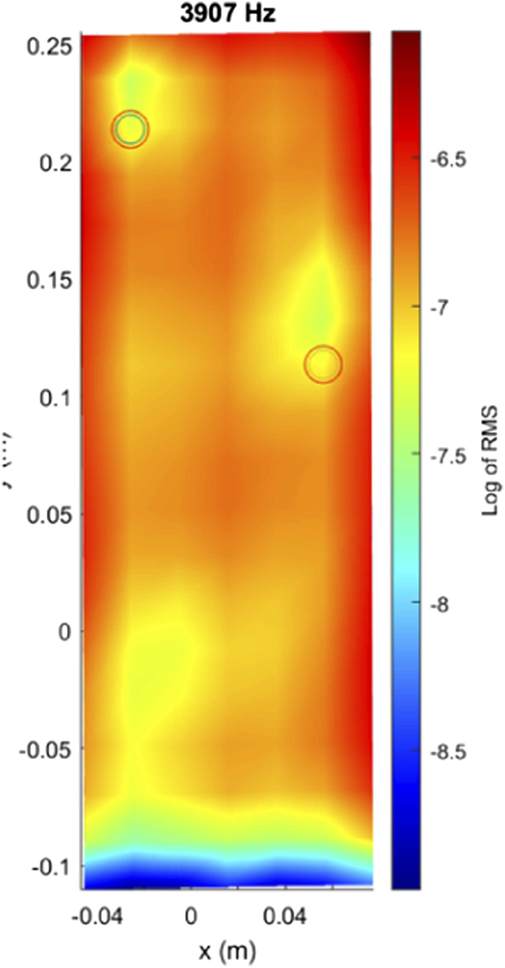

However, this approach has a major limitation: it only works when a sensor is located directly over or near the damage. In real-world applications, this is rarely feasible. Our objective is not to detect damage only where the sensor is placed, but rather to enable a sensor located anywhere on the structure to identify anomalies occurring in other areas. This is precisely the motivation for adopting a deep learning approach based on time-frequency representations, which captures complex patterns across the entire signal and allows for global detection from local measurements. This transition is what gives our methodology its practical value and innovation potential. In addition, only with certain frequencies will the approach be effective. In Figure 7, a different excitation frequency is employed. For the case where two bumpers are included (a), only one of them is detected.

Figure 7.

Log RMS (2792 Hz), misidentification of bumpers. (a) Two bumpers, (b) top bumper, (c) low bumper, (d) linear.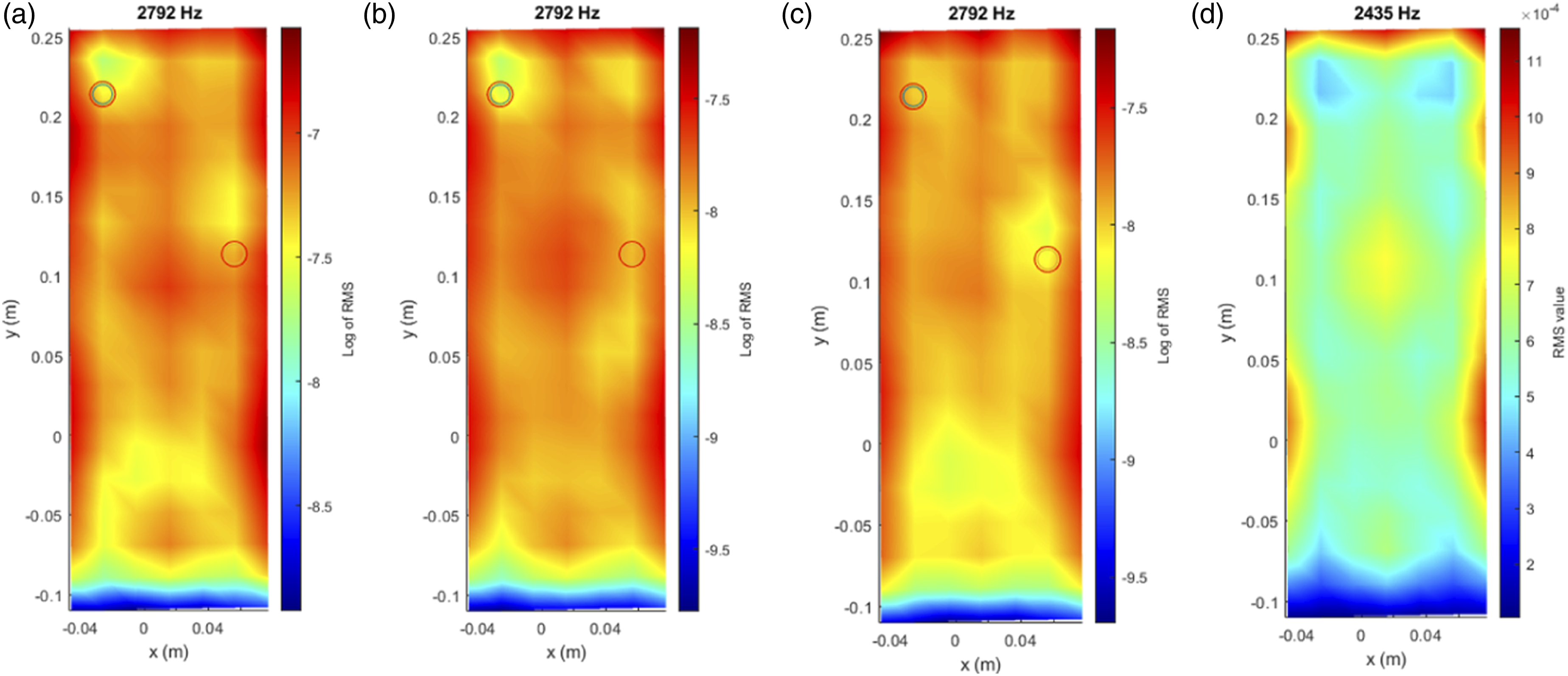

Figures 5–7 illustrate the results of this initial RMS-based analysis, using data from Nonlinear Set 3, where two bumpers were placed simultaneously. The plotted vibration signals across the surface clearly show how the presence and location of bumpers affect the dynamic response. These visualizations provided the foundation for validating the presence of meaningful signal variations prior to developing the classification model.

While RMS is not used directly as a feature in this study, it is still relevant because it reflects the overall energy of the signal. When damage is present, energy distribution can change (especially if the damage is near the sensor) causing variations in the RMS. Since the scalogram keeps both amplitude and frequency information, the model can still learn from energy changes in the signal, which helps in identifying and localizing potential damage.

Integrating deep learning with transfer learning

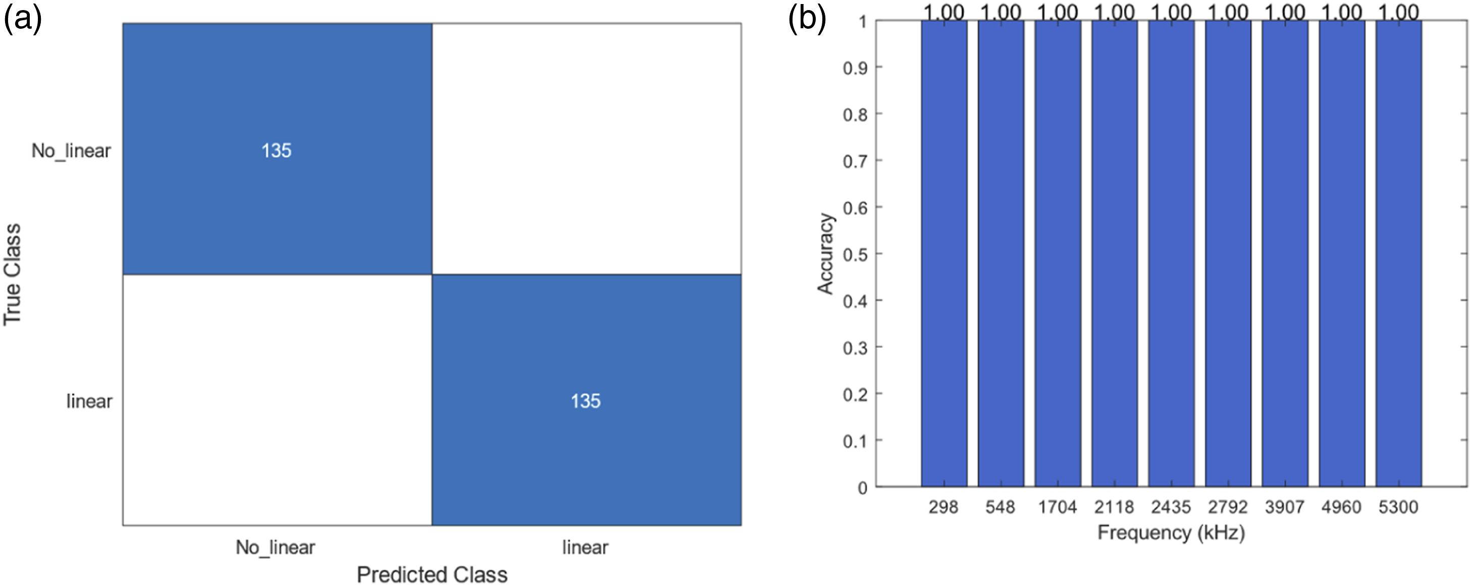
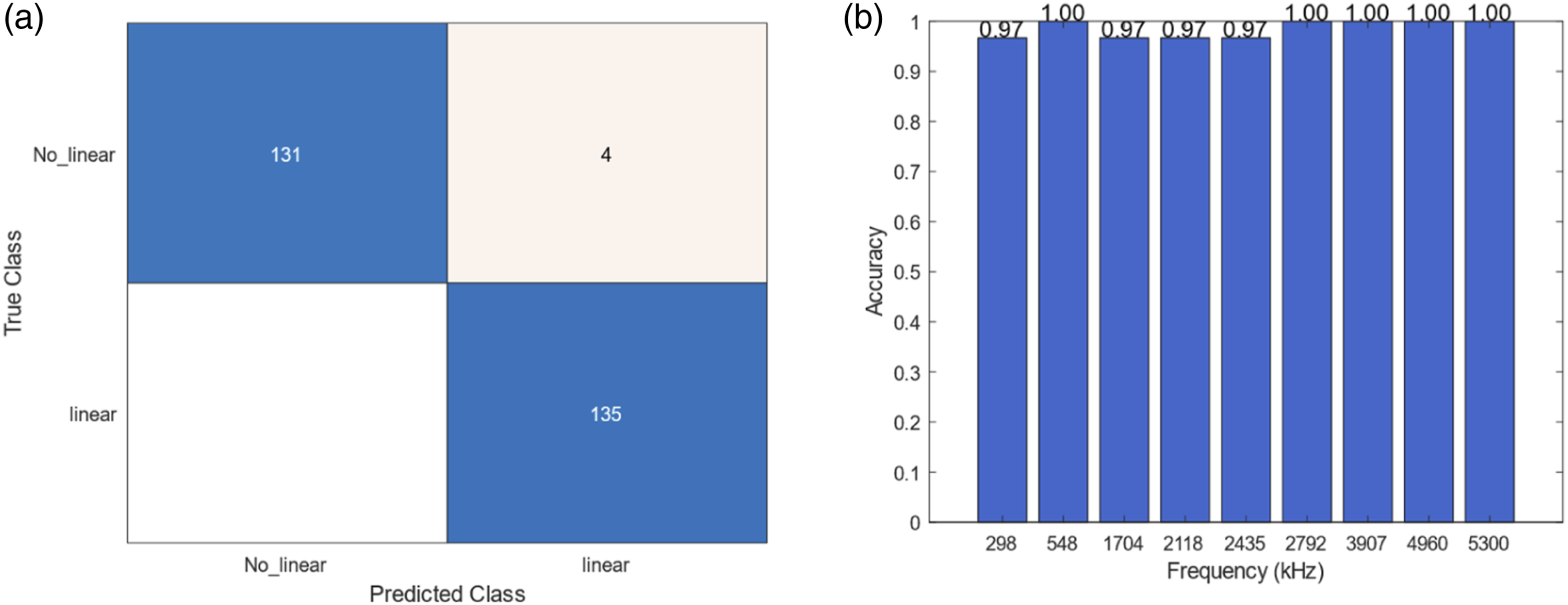
The core of the experimental design integrates the use of a neural network trained initially with data from the LDV and subsequently fine-tuned using data from new accelerometers located on the plate. This approach leverages transfer learning to adapt the neural network to accelerometer data, enhancing its applicability and reducing dependency on the more complex and expensive LDV setups. The accelerometers, more economical and easier to deploy, are tested in new configurations to ensure that the model can generalize from previously unseen data. Four new accelerometers were placed on the structure to collect new sets of data, with the training procedure excluding one accelerometer in each experimental iteration to test the ability of the model to generalize effectively (Figures 8–10).

Figure 8.

Location of accelerometers for the fine-tune and test de neural network.

Figure 9.

(a) Confusion matrix for case 1 and (b) accuracy of the model for each frequency.

Figure 10.

(a) Confusion matrix for case 2 and (b) accuracy of the model for each frequency.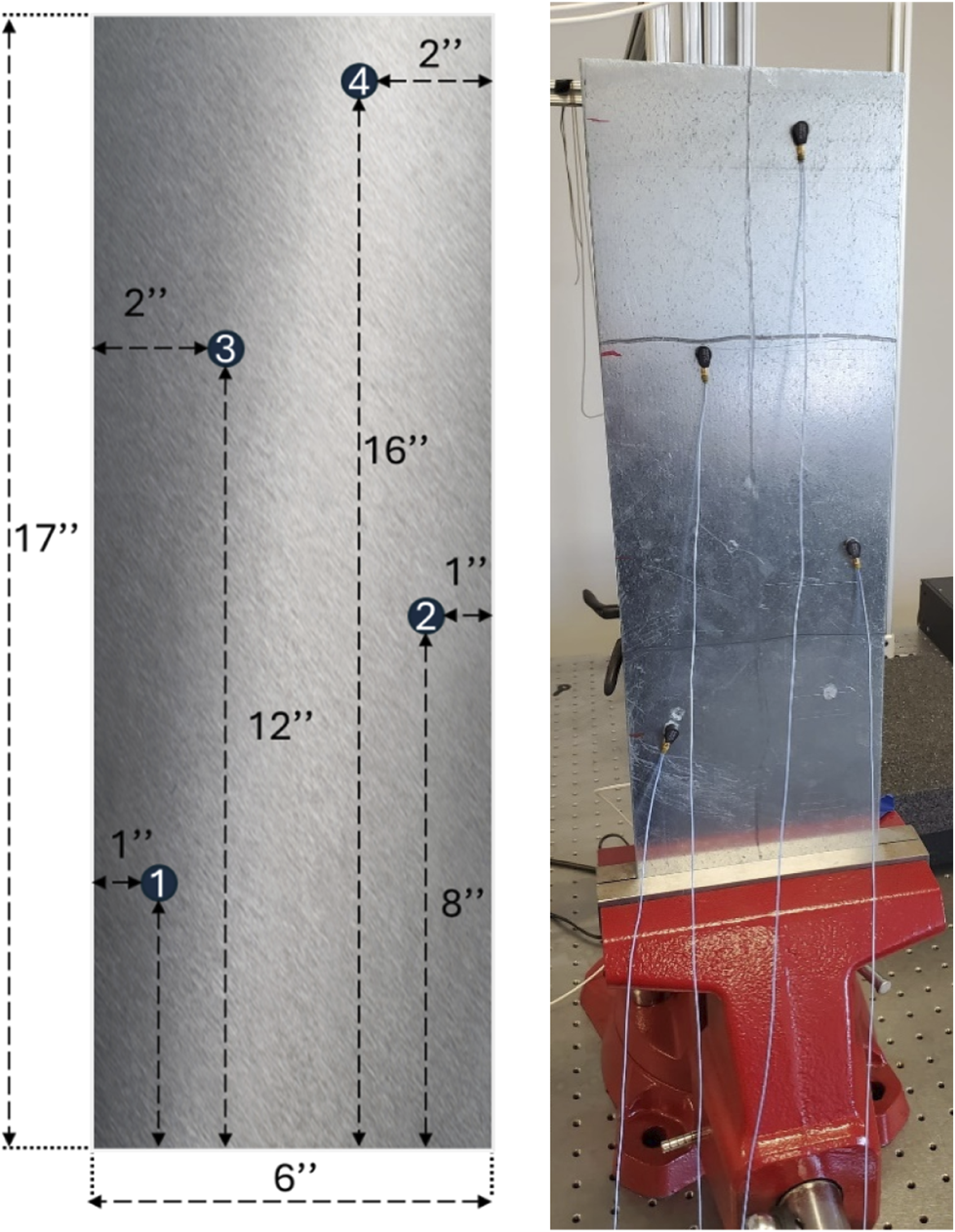

This setup included four distinct training scenarios:

• Case 1: Laser Doppler Vibrometer dataset combined with data from accelerometers 2, 3 and 4, tested against data from accelerometer 1.

• Case 2: LDV dataset combined with data from accelerometers 1, 3, and 4, tested against data from accelerometer 2.

• Case 3: LDV dataset combined with data from accelerometers 1, 2, and 4, tested against data from accelerometer 3.

• Case 4: LDV dataset combined with data from accelerometers 1, 2, and 3, tested against data from accelerometer 4.

These configurations were carefully planned to ensure that each training set was unique, preventing overfitting and validating the performance of the model across diverse data inputs.

Results

The evaluation of the performance of the neural network in classifying vibration signals based on the developed scalograms was conducted through a series of diverse designed test scenarios. These scenarios were structured to assess the ability of the model to distinguish between linear and nonlinear behaviors under varied conditions. The following subsections detail the outcomes of each specific case setup, highlighting the effectiveness of the model and areas where performance could potentially be enhanced.

Case 1

• Laser Doppler Vibrometer dataset combined with data from accelerometers 2, 3 and 4, tested against data from accelerometer 1.

In this scenario, the model was tasked with classifying signals using data from three accelerometers while being tested against the data from a fourth, previously unseen accelerometer. The results indicated a high accuracy in identifying nonlinear behavior. Figure 8, Figure 9(a) shows the confusion matrix for this case and Figure 9(b) shows the accuracy of the model for each frequency of the new data acquired with the accelerometer 1.

The network perfectly classifies cases with nonlinear behavior (135).

Case 2

• LDV dataset combined with data from accelerometers 1, 3, and 4, tested against data from accelerometer 2.

This case tested the robustness of the model by swapping the training and testing accelerometers, providing insights into the flexibility of the neural network in adapting to new data inputs. The results demonstrated consistent performance, with slight variations in the detection of linear states.

Case 3

• Case 3: LDV dataset combined with data from accelerometers 1, 2, and 4, tested against data from accelerometer 3.

The network classifies certain frequencies perfectly, with two misclassifications for high frequencies. Figure 11

Figure 11.

(a) Confusion matrix for case 3 and (b) accuracy of the model for each frequency.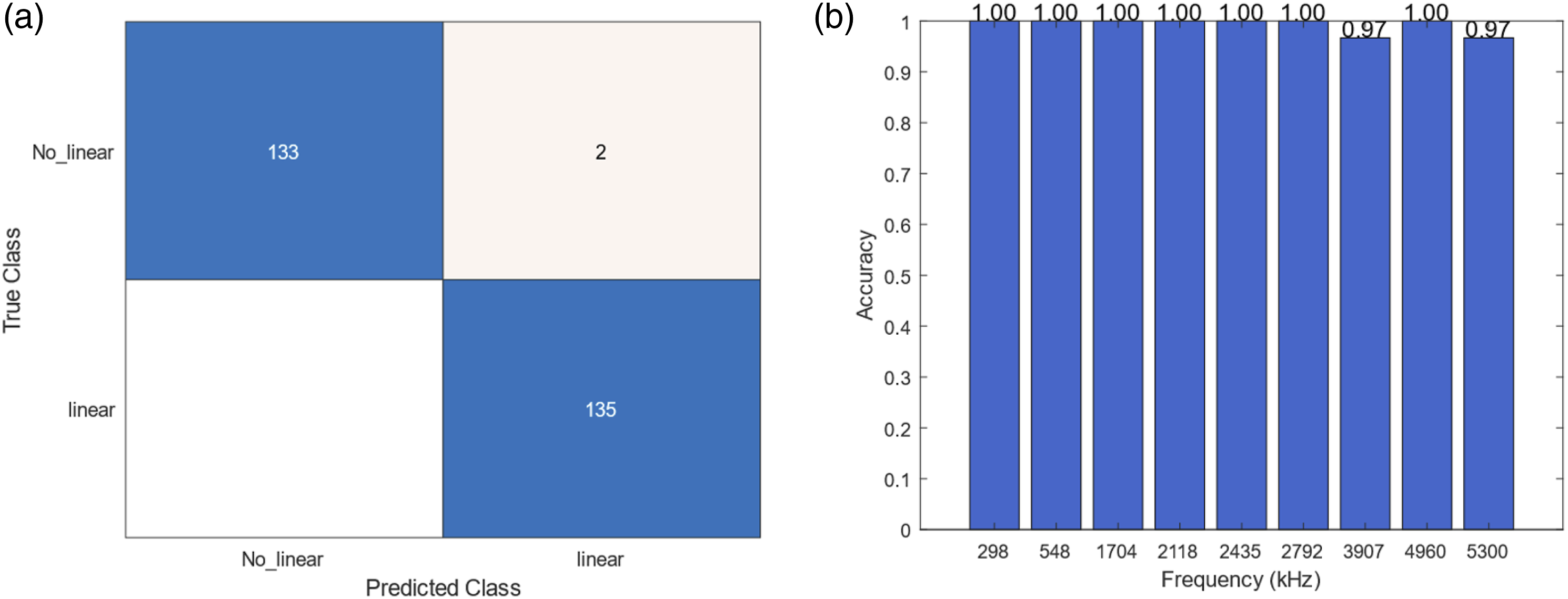

Case 4

• Case 4: LDV dataset combined with data from accelerometers 1, 2, and 3, tested against data from accelerometer 4.

The final test case reversed the roles of the previously used accelerometers, placing the model in a position to prove its comprehensive learning from the earlier scenarios. The outcome was a testament to the model’s learning depth, showing promising results in both linear and nonlinear vibration detection. Figure 12

Figure 12.

(a) Confusion matrix for case 4 and (b) accuracy of the model for each frequency.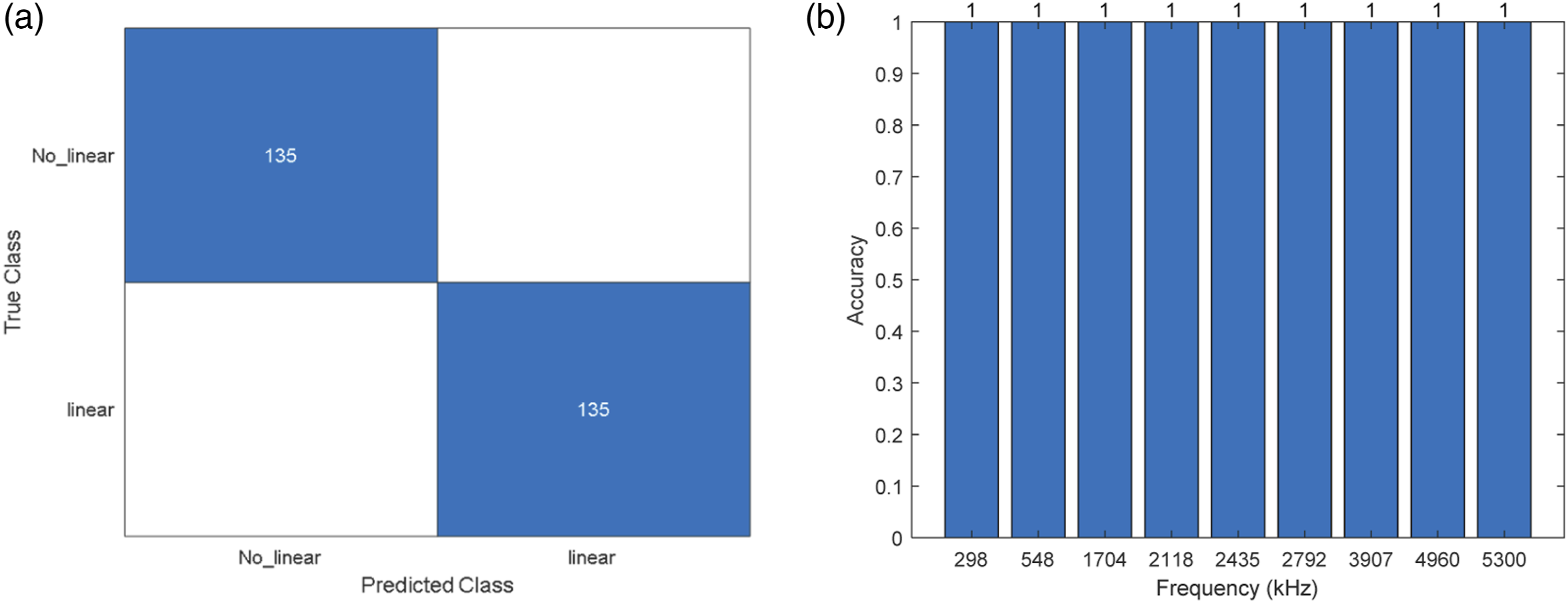

Overall model evaluation and comparation

To evaluate the effectiveness of different convolutional CNN architectures for vibration-based damage classification, a comparative analysis was conducted using GoogLeNet, ResNet, and SqueezeNet. Each model was trained and tested across the four previews cases using the same dataset and experimental conditions. The hyperparameters were selected to match the characteristics of each architecture while ensuring a fair comparison: ResNet was configured with a learning rate of 10⁻³ and batch size of 32, SqueezeNet used a learning rate of 10⁻⁴ and batch size of 15, and all models were trained for 20 epochs.

The results, shown in Figure 13, reveal that GoogLeNet consistently outperformed the other two architectures, especially in the more challenging cases. In Cases 1, 2 and 3, which include accelerometer data from sensors positioned closer to the shaker, both ResNet and SqueezeNet showed significantly lower accuracies (around 50% or even less) indicating that they struggled to distinguish the subtle effects produced by the bumpers in those regions. In contrast, GoogLeNet maintained very high accuracy, exceeding 98% in all three cases, including perfect classification in Case 1.

Figure 13.

Accuracy comparison of GoogleNet, ResNet, and SqueezeNet across four classification cases.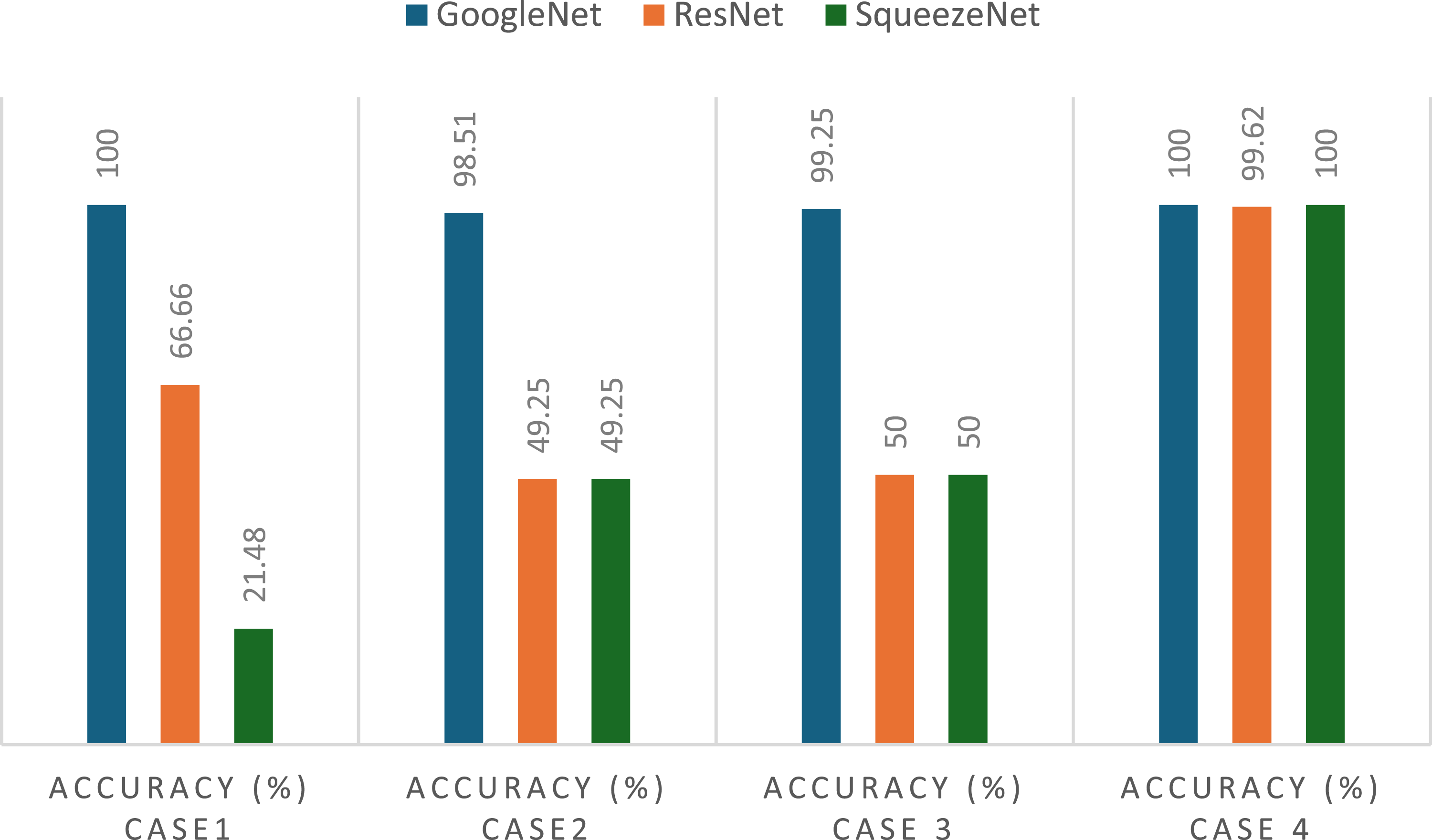

In Case 4, where the accelerometer is located farther from the shaker, all three architectures achieved high accuracy, close to 100%. This suggests that, in that region of the plate, the vibration patterns caused by the presence of bumpers are more pronounced, making it easier for any model to capture the differences between healthy and altered states.

These results confirm that not all sensor locations are equally informative, and that model robustness to these variations is crucial for general application.

The superior performance of GoogLeNet can be attributed to its inception modules, which extract features at multiple spatial resolutions, making the network better suited to the complex and variable patterns found in time-frequency scalograms. This architectural advantage, combined with its proven stability and accuracy in our tests, justifies its selection as the core architecture for the proposed structural health monitoring method.

Conclusion

In this study, we have introduced a new methodology for classifying vibration signals by effectively harnessing the capabilities of transfer learning and continuous wavelet transform analysis. We adapted the GoogLeNet architecture, which was originally developed for image classification, to analyze time-frequency representations of vibration signals transformed into RGB scalograms. This technique reduces the need for the extensive computational resources and large datasets typically required to train deep Convolutional Neural Networks from scratch. Moreover, it significantly improves the adaptability and operational efficiency of these networks within the new context of vibration signal analysis.

Our experiments with the modified GoogLeNet architecture have demonstrated its ability to differentiate between normal and anomalous vibration patterns. This distinction is crucial for advancing non-destructive testing methods, particularly within the field of structural health monitoring, where the early identification of potential issues is vital to prevent severe failures.

Considering the results presented, it also encourages the possibility of expanding the current method for a multiclass classification for different levels or location of damages. In addition, damage localization can be further explored for future research directions, considering the flexibility of the transfer learning approach, to enrich and increase the variation of possible scenarios, adding simulation data into the training dataset could allow a better performance model.

Finally, the application of deep transfer learning techniques in this study highlights a promising direction for enhancing the accuracy and accessibility of vibration signal classification. This novel approach is poised to contribute significantly to various engineering fields, particularly those involved in maintaining the integrity of infrastructure and machinery.

Future work

With advancements in computational technology, the generation and analysis of scalograms through deep learning models can be optimized to occur in near real-time. This analytical speed is essential in industries such as aerospace, automotive, and manufacturing, where structural integrity must be monitored continuously to ensure operational safety. Future developments could focus on increasing the computational efficiency of both the scalogram generation and the inference phase, enabling faster decision-making and failure prevention.

In addition to improving performance, the methodology presented in this study has shown scalability and flexibility, making it suitable for industrial deployment. One practical strategy would involve instrumenting a new component (known to be in good condition) with several accelerometers. The signals captured under normal operation would serve as a baseline, which could be used to align with the features learned by the pre-trained model through transfer learning. As the system continues to operate, any deviations from the baseline patterns could be detected and classified as potential defects, enabling real-time condition monitoring without retraining the entire network.

While generalization was evaluated using signals acquired on different days and from accelerometers not included in the training set, all tests were conducted on the same structure. Future research should include validation on different structural configurations and damage scenarios to assess the model’s robustness when facing new, unseen conditions.

Moreover, as fault detection and classification methods evolve, this framework allows for continuous model refinement through the integration of augmented datasets and operational feedback. This iterative learning approach would improve the model’s robustness and adaptability to new damage scenarios. Future research could explore the development of automated learning systems that self-update based on real-world performance, further enhancing long-term reliability in dynamic environments.

Another promising direction is to extend the approach to damage localization. Although the data is collected over a spatial mesh, localizing the bumper is not straightforward due to the influence of excitation frequency, vibration modes, and the fact that bumpers often affect multiple areas at once. As an alternative to classification, future work could explore regression-based models to estimate the approximate position of the disturbance, enabling more precise spatial monitoring.

Footnotes

Acknowledgments

This work was partially funded by the European Union’s Horizon 2020 research and innovation programme under the Marie Skłodowska-Curie grant agreement No. 777822.It was also partially supported by the project “ICARUS – Inspección y Control Automatizado con Redes Neuronales y UAVs en Sistemas Fotovoltaicos” [ref. SI4/PJI/2024-00233], funded by the Comunidad de Madrid through a direct grant for research and technology transfer at the Universidad Autónoma de Madrid.

ORCID iD

Carlos Quiterio Gómez Muñoz

Funding

The authors disclosed receipt of the following financial support for the research, authorship, and/or publication of this article: This project was partially funded by the European Union’s Horizon 2020 research and innovation programme under the Marie Skłodowska-Curie grant agreement No. 777822. It was also partially supported by the project “ICARUS – Inspección y Control Automatizado con Redes Neuronales y UAVs en Sistemas Fotovoltaicos” [ref. SI4/PJI/2024-00233], funded by the Comunidad de Madrid through a direct grant for research and technology transfer at the Universidad Autónoma de Madrid.

Declaration of conflicting interests

The authors declared no potential conflicts of interest with respect to the research, authorship, and/or publication of this article.

References

Arul

Kareem

. Data anomaly detection for structural health monitoring of bridges using shapelet transform. Smart Struct Syst 2022; 29: 93–103.

Tang

Chen

Bao

, et al. Convolutional neural network-based data anomaly detection method using multiple information for structural health monitoring. Struct Control Health Monit 2019; 26: e2296.

Khazaee

Derian

Mouraud

. A comprehensive study on Structural Health Monitoring (SHM) of wind turbine blades by instrumenting tower using machine learning methods. Renew Energy 2022; 199: 1568–1579.

Kalimullah

NMM

Shelke

Habib

. A deep learning approach for anomaly identification in PZT sensors using point contact method. Smart Mater Struct 2023; 32: 095027.

Sabato

Dabetwar

Kulkarni

, et al. Noncontact sensing techniques for AI-aided structural health monitoring: a systematic review. IEEE Sens J 2023; 23(5): 4672–4684.

Kapteyn

Willcox

. From physics-based models to predictive digital twins via interpretable machine learning, arXiv preprint arXiv:2004.11356, 2020.

Qian

Kramer

Peherstorfer

, et al. Lift & learn: physics-informed machine learning for large-scale nonlinear dynamical systems. Phys Nonlinear Phenom 2020; 406: 132401.

Malekloo

Ozer

AlHamaydeh

, et al. Machine learning and structural health monitoring overview with emerging technology and high-dimensional data source highlights. Struct Health Monit 2022; 21(4): 1906–1955.

Lim

Yong

KSC

Lau

, et al. Future of generative adversarial networks (GAN) for anomaly detection in network security: a review. Comput Secur 2024; 139: 103733.

10.

Iamsumang

Mosleh

Modarres

. Hybrid DBN monitoring and anomaly detection algorithms for on-line SHM. In: 2015 61st Annual Reliability and Maintainability Symposium (RAMS 2015), 2015; IEEE.

11.

Kromanis

Kripakaran

. Performance of signal processing techniques for anomaly detection using a temperature-based measurement interpretation approach. J Civ Struct Health Monit 2021; 11: 15–34.

12.

Yun

C-B

Wan

H-P

, et al. Probabilistic principal component analysis-based anomaly detection for structures with missing data. Struct Control Health Monit. 2021; 28: e2698.

13.

Liu

, et al. A deep learning-based method for automatic abnormal data detection: case study for bridge structural health monitoring. Int J Struct Stabil Dynam. 2023; 23: 2350131.

14.

Kim

S-Y

Mukhiddinov

. Data anomaly detection for structural health monitoring based on a convolutional neural network. Sensors 2023; 23: 8525.

15.

Liu

Niu

Zhao

, et al. Data anomaly detection for structural health monitoring using a combination network of GANomaly and CNN. Smart Struct Syst 2022; 29: 53–62.

16.

Barzegar

Laflamme

, et al. Ensemble of recurrent neural networks with long short-term memory cells for high-rate structural health monitoring. Mech Syst Signal Process 2022; 164: 108201.

17.

Shang

Sun

Liu

, et al. Defect-aware transformer network for intelligent visual surface defect detection. Adv Eng Inform 2023; 55: 101882.

18.

Boffa

Arena

Monaco

, et al. About the combination of high and low frequency methods for impact detection on aerospace components. Prog Aero Sci 2022; 129: 100789.

19.

Yang

Mei

Song

, et al. Transfer-learning-based online mura defect classification. IEEE Trans Semicond Manufact 2018; 31: 116–123.

20.

Guan

Bao

, et al. Pattern recognition based on time-frequency analysis and convolutional neural networks for vibrational events in φ-OTDR. Opt Eng 2018; 57: 1.

21.

Daubechies

. The wavelet transform, time-frequency localization and signal analysis. IEEE Trans Inf Theory 1990; 36: 961–1005.

22.

Ren

Qian

Zhang

, et al. Deep scalogram representations for acoustic scene classification. IEEE/CAA J Autom Sinica 2018; 5: 662–669.

23.

Manjunath

Tewary

Khatri

, et al. In-process monitoring of the ultraprecision machining process with convolution neural networks. Int J Comput Integrated Manuf 2024; 37: 37–54.

24.

Manjunath

Tewary

Khatri

, et al. Monitoring of machining process anomalies in diamond turning of Ti6Al4V alloy using transfer learning-based algorithms. Comput Ind Eng 2023; 182: 109359.

25.

Wan

Yang

Huang

, et al. A review on transfer learning in EEG signal analysis. Neurocomputing 2021; 421: 1–14.

26.

Caballol

Raposo

Gil-Carrillo

. Non-destructive testing of concrete layer adhesion by means of vibration measurement. Constr Build Mater 2024; 411: 134548.

27.

Salehi

Bagherzadeh

Fakhari

. Experimental detection of train wheel defects using wayside vibration signal processing. Struct Health Monit Int J. 2023; 22(5): 3286–3301.

28.

Ahmed

Ahmad

Chehri

, et al. A smart-anomaly-detection system for industrial machines based on feature autoencoder and deep learning, Micromachines 2023; 14: 154.

29.

Zhao

Sun

, et al. Applications of machine learning in real-time control systems: a review. Meas Sci Technol. 2024; 36(1): 012003.

30.

Chen

Yang

Xue

, et al. Deep transfer learning for bearing fault diagnosis: a systematic review since 2016. IEEE Trans Instrum Meas 2023; 72: 1–21.

31.

Zhang

Qin

, et al. A systematic review of deep transfer learning for machinery fault diagnosis. Neurocomputing 2020; 407: 121–135.

32.

Gong

Shao

Luo

, et al. A deep transfer learning model for inclusion defect detection of aeronautics composite materials. Compos Struct 2020; 252: 112681.

33.

Sai

Venkatesh

Dhanasekaran

, et al. Transfer learning based fault detection for suspension system using vibrational analysis and radar plots. Machines 2023; 11: 778.

34.

Zhao

Sun

, et al. Few-shot transfer learning for intelligent fault diagnosis of machine. Measurement 2020; 166: 108202.

35.

Huang

, et al. A perspective survey on deep transfer learning for fault diagnosis in industrial scenarios: theories, applications and challenges, Mech Syst Signal Process 2022; 167: 108487.

36.

Szegedy

Liu

Jia

, et al. Going deeper with convolutions. In: Proceedings of the IEEE conference on computer vision and pattern recognition, 2015, pp. 1–9; IEEE.

37.

Moll

Kathol

Fritzen

, et al. Open guided waves: online platform for ultrasonic guided wave measurements. Struct Health Monit 2019; 18(5-6): 1903–1914.

38.

Moll

Kexel

Kathol

, et al. Guided waves for damage detection in complex composite structures: the influence of omega stringer and different reference damage size. Appl Sci 2020; 10(9): 3068.

39.

Pawel

Maciej

Maria

, et al. Dataset on full ultrasonic guided wavefield measurements of a CFRP plate with fully bonded and partially debonded omega stringer. Data Brief 2022; 42: 108078.

Structural health monitoring through deep learning: A study on scalogram-based vibration signal classification

Abstract

Keywords

Introduction

Methodology

Preparation and creating time-frequency representations

Transfer learning strategy

Training the vibration signal classifier

Case studies

Scenario 1: Linear vibration analysis

Scenario 2: Introducing nonlinearities with bumpers

Frequency selection and experimental design

Integrating deep learning with transfer learning

Results

Case 1

Case 2

Case 3

Case 4

Overall model evaluation and comparation

Conclusion

Future work

Footnotes

Acknowledgments

ORCID iD

Funding

Declaration of conflicting interests

References