Enhancing beam structural damage detection using spectral moment values and spectral moment cumulative function models

Abstract

Evaluation and identification of structural damage play a crucial role in ensuring the safety and reliability of structures. This study explores the application of spectral moment value analysis as a robust tool to assess and detect structural damage. Spectral moment values provide detailed information on how a structure responds to load, helping to accurately identify the location, type, and extent of the damage. By monitoring changes in spectral moment values using experimental data on damaged and undamaged steel beams under moving loads, early signs of hidden damage can be detected, allowing timely implementation of repair or maintenance measures before the condition worsens. Moreover, spectral moment value analysis supports the evaluation of structural reliability based on load bearing capacity and resistance to damage, aiding in decision-making processes regarding the repair, improvement, or replacement of the structure. The methodology used in this research provides a cost-effective and efficient approach to the evaluation and identification of structural damage, with potential applications in various engineering fields.

Introduction

The evaluation and monitoring of structural damage play a crucial role in ensuring the safety and maintaining the operational efficiency of civil engineering and construction projects. In particular, the early-stage detection of small defects can be challenging, but if left undetected and untreated, these defects can progress, leading to significant degradation and compromising the safety and durability of structures. Advances in structural health monitoring have been driven by the development of mathematical analysis models and sensor technology. However, traditional methods still face limitations in detecting early damage and accurately quantifying its extent and location

This study presents a novel approach using spectral moment value analysis and the cumulative spectral moment function model to assess and identify damage in beam structures. Spectral moment values are essential statistical parameters that reflect the energy distribution of a signal across various frequency bands, enabling a detailed evaluation of structural responses under load. The application of spectral moments allows for the detection of subtle changes in the frequency response of a structure—an important factor in identifying damage.

A key feature of this research is the development and experimental validation of the cumulative spectral moment value model, which enables the tracking of energy shifts as damage progresses over time. Using measured data from tests conducted on damaged and undamaged steel beams, the study demonstrates the capability to detect early signs of potential damage through shifts in energy from high to low-frequency regions. This model allows for the precise identification of damage location and severity and supports early interventions for maintenance and repair.

The proposed method offers cost and time efficiency compared to previous studies by utilizing controlled laboratory conditions for testing. This approach provides practical advantages for broad implementation in structural health monitoring across various types of structures. The results confirm that both the spectral moment value and cumulative spectral moment models are powerful and sensitive tools for detecting and monitoring structural damage, contributing to improved reliability and lifespan of engineering structures. The advantages of moment spectral analysis over other methods are shown to include:

- Enhanced sensitivity to early damage detection: Spectral moment analysis, particularly through zeroth-order spectral moments (M0), provides heightened sensitivity to subtle changes in the energy distribution across frequency bands. This sensitivity allows for the detection of damage in its early stages, which is often challenging for traditional methods such as modal analysis or acoustic tomography. These traditional methods typically rely on noticeable shifts in modal frequencies or acoustic properties, which may not occur until damage has progressed significantly. In contrast, spectral moment analysis captures energy shifts early on, enabling proactive maintenance to prevent further structural deterioration.

- Cost-Effective Implementation and Simplicity: Unlike acoustic tomography, which requires specialized equipment such as advanced transducers and computationally intensive imaging techniques, spectral moment analysis relies on standard vibration sensors and straightforward signal processing algorithms. This significantly reduces both the cost of deployment and the level of technical expertise required for operation. By leveraging readily available tools, spectral moment analysis becomes a more practical and economical option for structural health monitoring, particularly for small- to medium-scale applications.

- Precision in localizing damage: Spectral moment analysis is highly effective in pinpointing the exact location of structural damage by analyzing the redistribution of energy in specific frequency zones. While modal analysis provides valuable insights into the global behavior of structures, its precision in detecting localized damage often depends on the density and placement of sensors. In contrast, spectral moment analysis, when combined with an optimized sensor network, offers precise localization without the need for extensive instrumentation, making it a more efficient alternative.

- Real-Time Monitoring Capability: The computational simplicity of spectral moment models facilitates their application in real-time monitoring scenarios. The ability to process vibration data rapidly allows for continuous structural health assessments, even under dynamic loading conditions. In comparison, acoustic tomography often requires significant post-processing of raw data to reconstruct detailed images, which can delay critical decision-making processes in real-time applications.

- Robustness to environmental noise: Spectral moment analysis exhibits a higher resilience to noise compared to acoustic methods, which are sensitive to environmental interference such as wind, traffic, or ambient vibrations. By focusing on energy distribution patterns within the frequency domain, this approach minimizes the influence of external noise, ensuring reliable detection of structural anomalies even in complex operational environments.

- Flexibility across linear and nonlinear problems: One of the unique advantages of spectral moment analysis is its applicability to both linear and nonlinear problems. The method can capture complex physical phenomena, such as the redistribution of energy from higher to lower frequency zones, which are often overlooked by traditional methods. This adaptability enables spectral moment analysis to address a wider range of structural conditions, including those involving irregular or evolving damage patterns.

- Integration with cumulative models for damage progression: The cumulative spectral moment model proposed in this study builds upon the fundamental advantages of spectral moment analysis. By aggregating spectral moment values over time, this model provides a detailed understanding of how damage progresses within a structure. The cumulative approach not only enhances the sensitivity of damage detection but also allows for precise tracking of damage evolution, offering critical insights for implementing predictive maintenance strategies.

Spectral moment analysis offers distinct advantages over traditional methods such as modal analysis and acoustic tomography. Its sensitivity to early damage, cost-effectiveness, precision in localization, real-time applicability, robustness to noise, and flexibility make it a superior choice for structural health monitoring. Furthermore, the integration of cumulative spectral moment models strengthens its utility by enabling detailed tracking of damage progression. These attributes align with the objectives of this study and demonstrate the potential of spectral moment analysis to revolutionize the field of structural health monitoring, providing a scalable, reliable, and efficient tool for ensuring structural safety and longevity.

Literature review

In the realm of civil engineering, the comprehensive assessment and continuous monitoring of structural damage are imperative to safeguard the integrity, longevity, and operational performance of structures, ensuring they remain resilient and secure under varying conditions and external stressors.^1,2 Current structural health monitoring^3,4 has made significant progress, driven by the development of mathematical models. Currently, models for assessing and monitoring structural damage and observation from space^5,6 in real world settings are summarized as depicted in Figure 1. Each assessment model addresses certain issues that the authors have resolved while also highlighting areas for further development in subsequent research efforts.

Figure 1.

Key models in structural damage assessment and monitoring.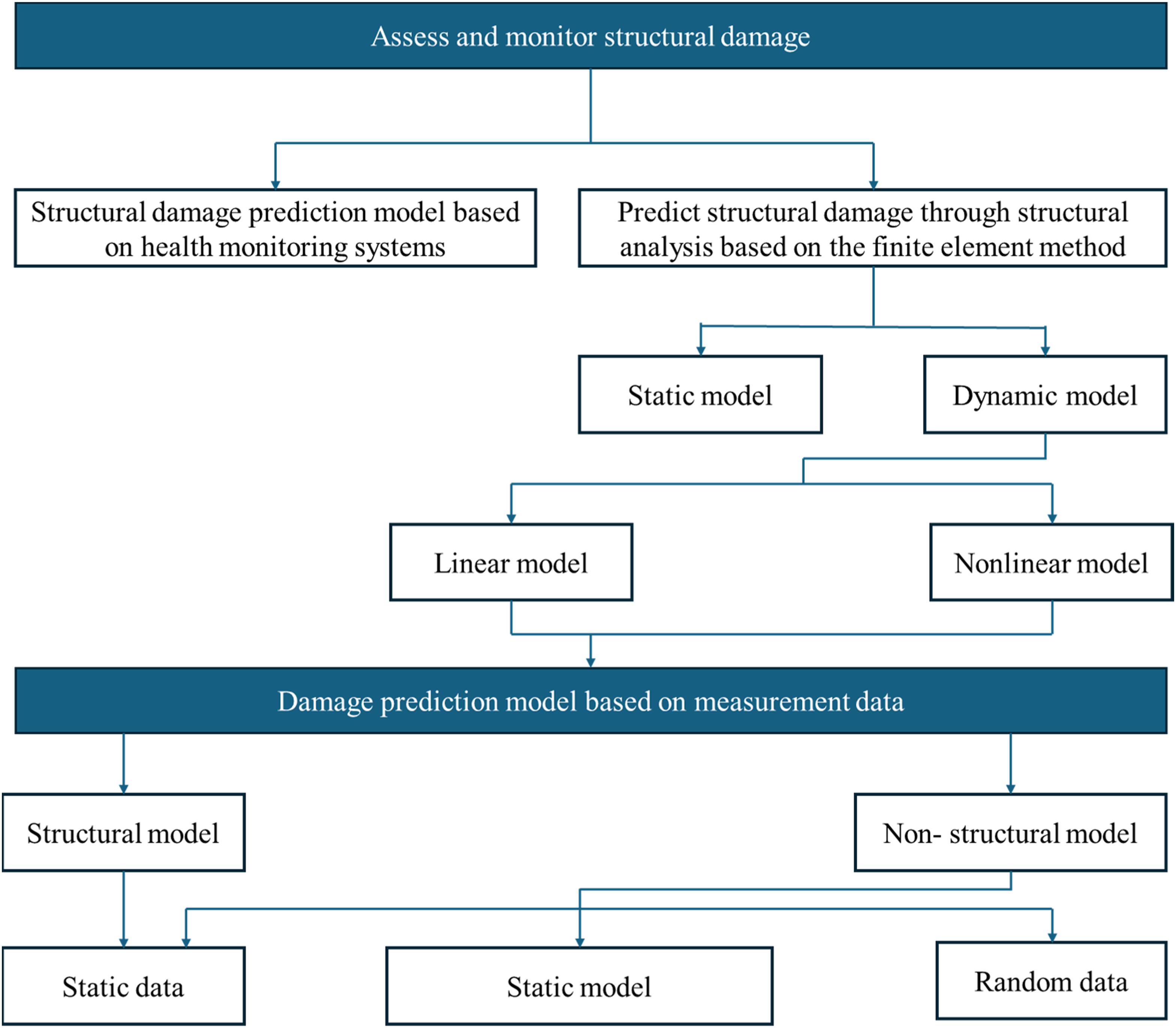

Figure 1 outlines a comprehensive framework for assessing and monitoring structural damage, structured into two main segments: the damage assessment process and the predictive modeling of damage using measurement data. The upper section details strategies for monitoring damage, including sensor-based approaches and analytical models. These methods support the development of advanced techniques, such as data-driven models and finite element analysis (FEA)-based models, which refine and enhance the monitoring capabilities. The lower section of the Figure 1 highlights the damage prediction model, which emphasizes the use of collected measurement data—such as vibration signals and structural responses—to forecast the health of the structure. By inputting this data into predictive models, future damage can be anticipated, thereby guiding proactive maintenance and repair decisions. This framework illustrates the workflow and interconnectedness of damage detection and predictive modeling techniques, showcasing how the incorporation of measurement data contributes to improved accuracy and reliability in structural health evaluation. In the context of this research, the emphasis on spectral moment analysis and cumulative spectral moment models demonstrates the importance of integrating precise measurement data for assessing changes in energy distribution across frequency zones. This approach not only enhances damage detection but also offers a method for tracking damage evolution, thus aligning with the goal of advancing structural health monitoring through robust analytical tools.

Among these methods, the data-driven damage prediction model stands out as the most advanced method currently to evaluate and forecast structural health.^7–9 It is evident that by this method numerous features are extracted from measured data combined with machine learning^10,11 and deep learning^12,13 algorithms to automate the analysis of real-world sensors data,^14,15 as detailed in Figure 2. Consequently, machine learning and deep learning enable the model^16–18 to learn from historical and current data to predict future damage conditions.^2,3,19 Based on the historical data on which the model has been trained,^3,20 potential future damage ²¹ can be predicted and classified and the developmental trends of these damages can be found. Due to its predictive capacity, this method improves the safety and performance of beam structures^22–24 by detecting and preventing potential problems before they become severe.^25,26 The combination of machine learning and deep learning with the ability to analyze diverse data makes this model a powerful and flexible tool for managing and maintaining structures. Figure 2 illustrates a flowchart showcasing how deep learning models are integrated into the structural damage detection process. The diagram begins with three primary input pathways, each representing distinct methods of data collection or analysis. These inputs converge into a single pathway that is processed through several stages, marked by a red-dotted box to signify the addition of deep learning models. This highlighted section emphasizes the core contribution of the study: the integration of deep learning into the existing structural damage detection framework. Each stage in this pipeline, depicted by blocks with downward-pointing arrows, represents a step in the sequential data processing. This layered approach enables a comprehensive analysis, allowing the deep learning model to iteratively learn from the input data and refine its predictive capabilities. By incorporating deep learning, the method enhances the accuracy and depth of traditional models, leading to more precise identification and prediction of structural damage. This innovative addition results in improved damage detection, showcasing the study’s significant advancement in bridging conventional analysis with modern deep learning techniques for superior structural health monitoring.

Figure 2.

Some parameters extracted from measured data in structural damage.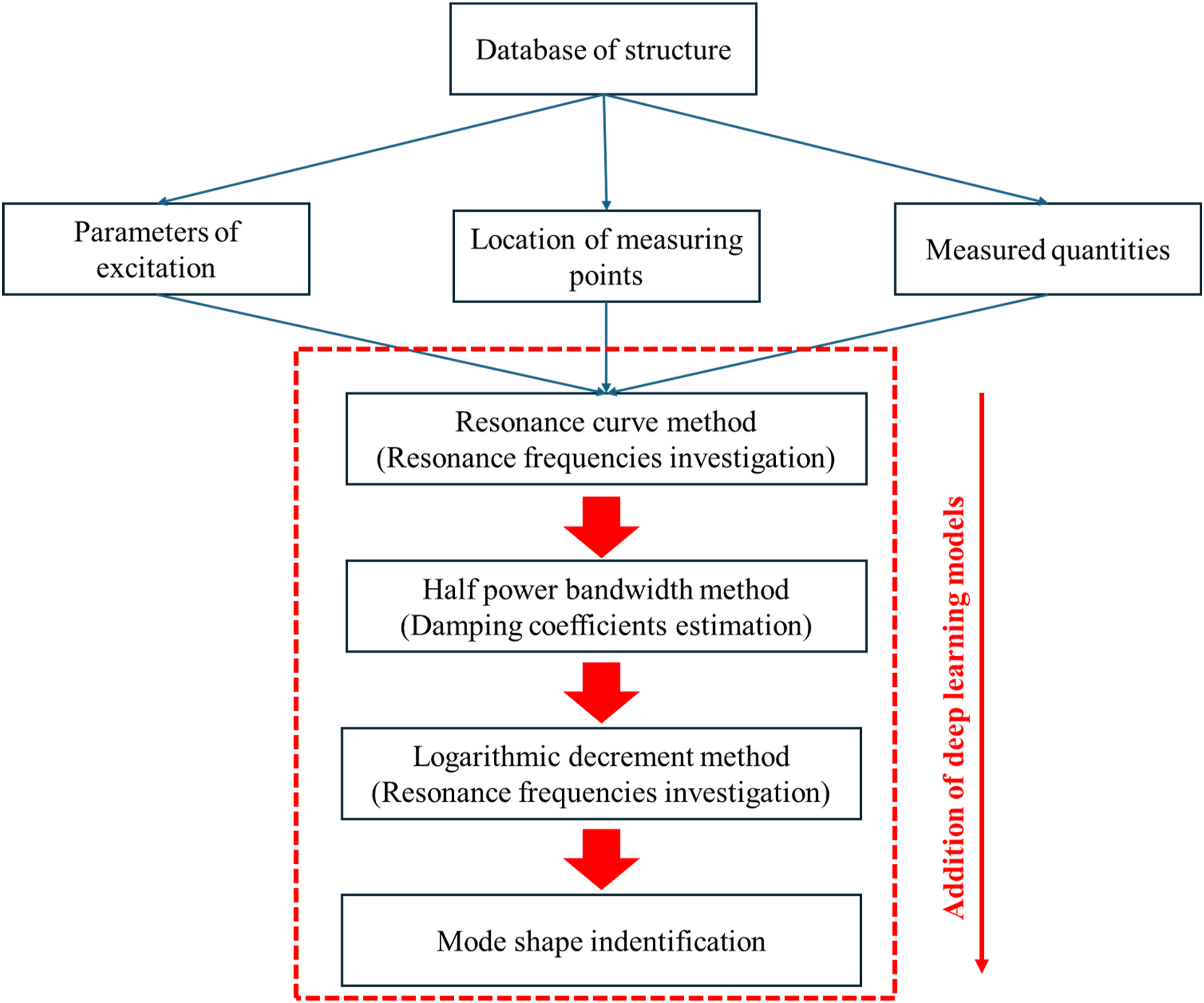

In addition to the data-driven structural damage assessment and prediction method,^27,28 the finite element analysis-based structural damage prediction model^29,30 is also an important method in civil engineering and mechanics. This model can be developed to predict and assess the condition of structures through numerical analyses and optimization algorithms.^31–33 The strength of this model is its ability to accurately and comprehensively calculate issues related to mechanics and material strength by modeling actual damages in the virtual environment of computers.^34–36 Using the finite element method,^37,38 the model can accurately simulate the loads and pressures on the structure. Another advantage of this model is its flexibility in application to various types of structures,^39,40 from bridges to high-rise buildings,^41,42 and industrial machinery. This facilitates its widespread application in various fields of engineering and technology. Furthermore, the model can interact and correlate with real-world data, providing important and accurate information on the actual performance of the structures, as shown in Figure 4. This makes the forecasting and evaluation process more accurate and reliable. However, it is important to note that deploying this method requires deep knowledge and high technical skills from researchers and engineers.^43–45 In addition, continuous updates on the data and computational methods are needed to ensure the effectiveness and reliability of the model in real-world environments. The finite element analysis-based structural damage prediction model is an important and useful tool to ensure the safety and performance of technical structures. With its accurate and flexible predictive capacity, this model is becoming an indispensable tool in the fields of engineering and construction. Figure 3 depicts the process of identifying structural defects through the Finite Element Method (FEM). This diagram features input data from multiple sources on both sides, converging into a central process. This process functions as the primary analysis mechanism for detecting structural irregularities. The outputs of the FEM analysis are shown on the right side, divided into various categories that represent different types of detected structural defects. The arrows indicate the flow of data from the initial input parameters through the FEM analysis process, leading to the classification and identification of specific defects. This figure underscores the significance of FEM in efficiently processing a wide range of input data to deliver a thorough evaluation of structural integrity. It showcases how FEM acts as an essential tool in structural health monitoring, capable of providing detailed insights that enhance the accuracy of damage detection and contribute to informed decision-making for maintenance and repair strategies.

Figure 3.

Overview of the finite-element analysis-based structural analysis model.

Figure 4.

Structural damage prediction model based on structural health monitoring systems.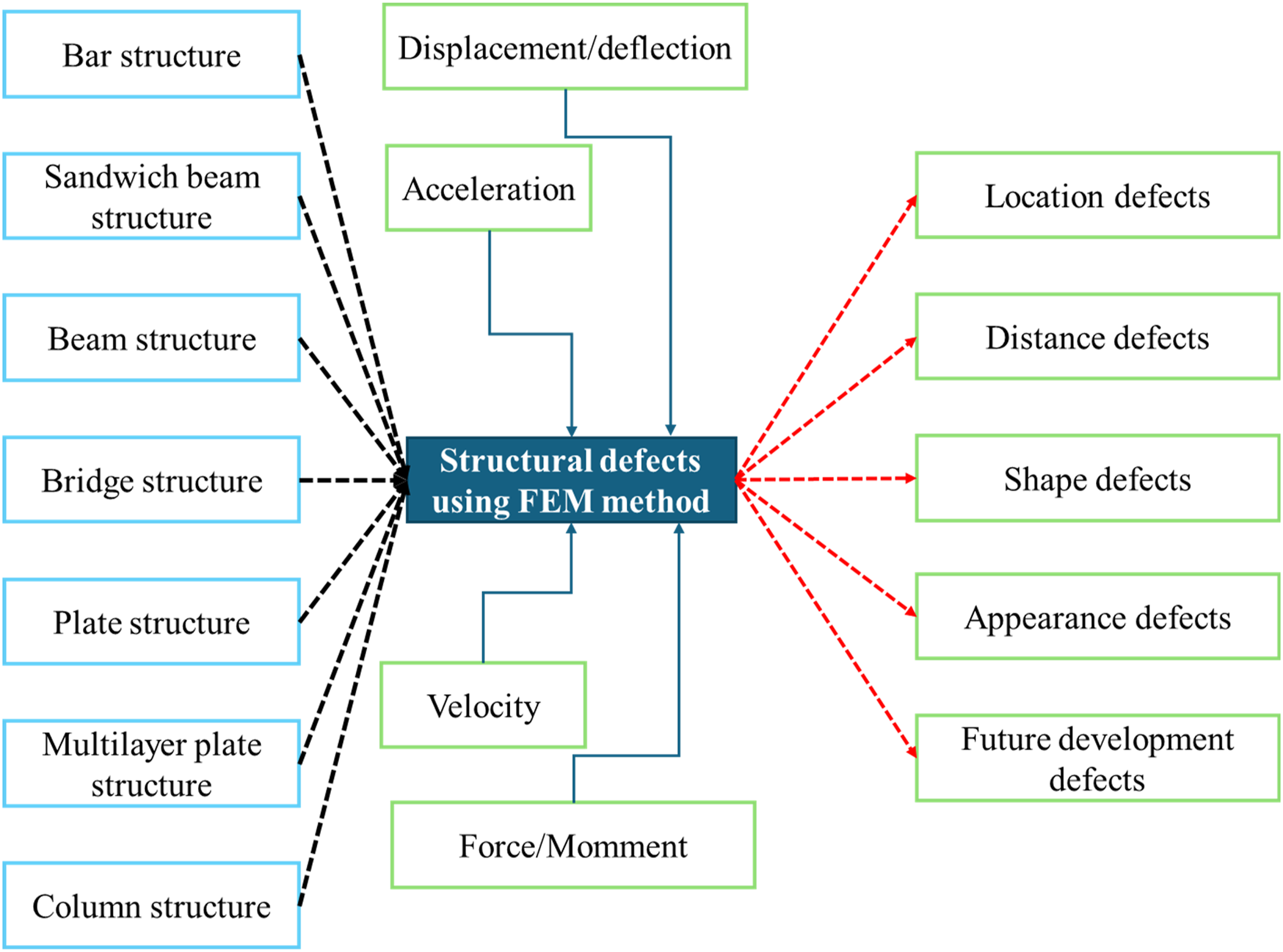

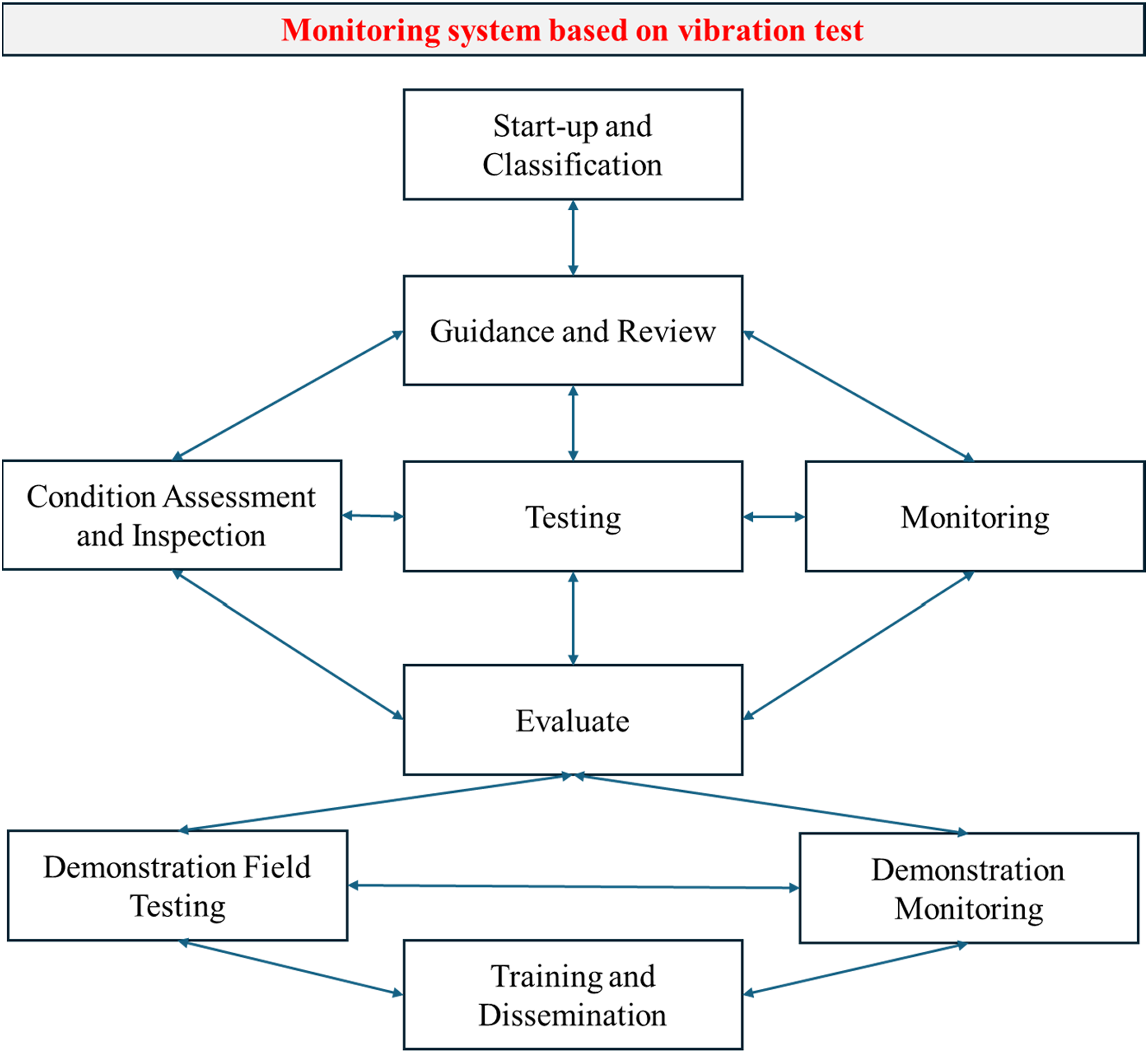
The structural damage prediction model based on structural health monitoring systems^46,47 represents a significant advancement in the field of infrastructure management and maintenance, as illustrated in Figure 4. By integrating sensor technologies,^31,48 data, and intelligent analysis, this model provides the ability to predict and prevent damage issues effectively and quickly. The strength of this model is its ability to continuously and uninterrupt monitoring of fundamental factors such as vibration,^49–51 pressure, temperature, and material strain.^52–54 Through directly integrated sensor systems within the structure^,55,56 the model collects real-time data and analyzes patterns to detect early signs of damage. ⁵⁷ Additionally, the model can also use artificial intelligence and machine learning to analyze and predict the tendency of damage based on historical data and predictive modeling. This facilitates decision-making based on accurate and predictive data, optimizing maintenance processes, and reducing costs. By promptly detecting and addressing damage issues, the model helps minimize the risk of accidents and incidents while improving the continuous operation capability of the system. However, deploying this model requires investment in both hardware and software, as well as a deep understanding of the relevant principles and techniques. Additionally, a strict monitoring and maintenance process is necessary to ensure the stability and effectiveness of the model over the long term. In conclusion, the structural damage prediction model based on structural health monitoring systems is an important and effective tool in the management and maintenance of infrastructure and construction projects. With its ability to continuously monitor and predict future events, this model offers many benefits in terms of safety, performance, and cost effectiveness.

The characteristics most commonly used in current research are depicted in Table 1. Depending on each approach, the studies extract parameters that reflect the relationship of changes within the structure.

Table 1.

Approaches and characteristics for damage assessment.

Directions of approach		Characteristics
Private status	Frequency	Fundamental frequency49–51
		Optimization of residual force52–54
	Shape function	Change in shape function 13
		Deformation energy55,56
		Derivative of the shape function58–60
	Damping	Instantaneous damping coefficient1,2
		Average damping coefficient61–63
Matrix method	Hardness matrix	Optimal technique16–18
		Adjust the structural model43,64
	Softness matrix	Dynamic softness43–45
Machine learning techniques (artificial intelligence)	Genetic Algorithm-GA)	Optimize hardness10,11
		Minimize the objective function65–67
	Artificial neural Network-ANN	Training the backpropagation network68,69
		Delay neural network 20
		System identification using ANN3,21
Signal analysis	Time domain	Statistical model70,71
	Time-frequency domain	Wavelet analysis31–33
	Frequency domain	Frequency response function (FRF) 37
		Power spectral density (PSD)14,71,72
		Spectral moment (M) 73

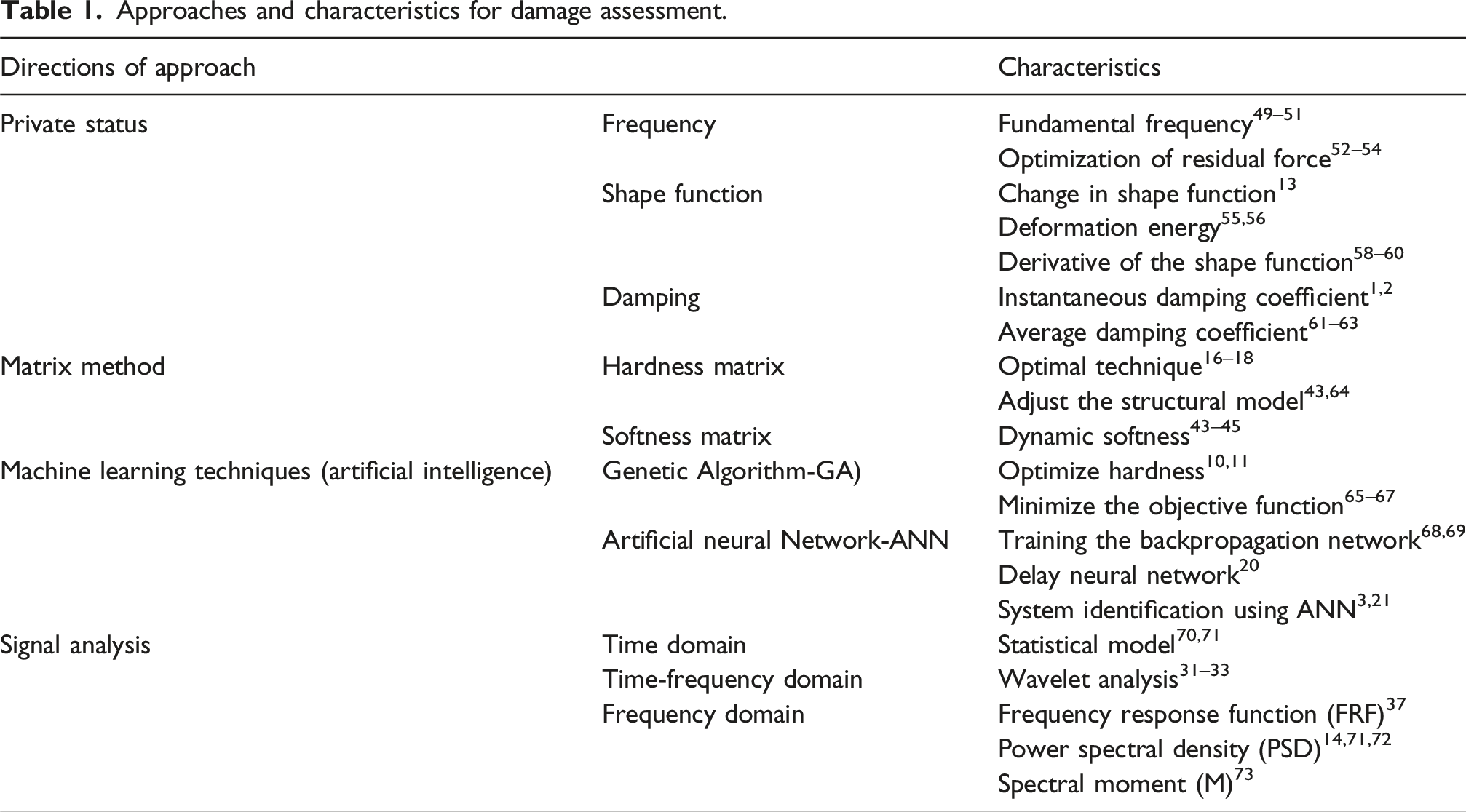
Signal spectrum analysis is a crucial method to analyze signals from monitoring devices attached to structures exhibiting signs of damage.^49–51 Using tools such as Fourier transform and wavelet analysis,^31,32 signals are transformed from the time domain to the frequency domain, ³⁷ enabling us to detect and analyze variations in the signal and changes in the spectral shape. ⁷³ Through signal spectrum analysis,^14,71 we can identify manifestations of damage within structures. Abnormal changes in the signal can indicate fractures, cracks, or large deformation of the material. This is particularly useful for identifying weaknesses or potential problems within structures before they lead to possible destructive consequences. By monitoring changes in the signal spectrum, ⁷² the state of structural damage can be assessed. This allows the prediction of incidents and the implementation of timely repair or maintenance measures to prevent major accidents. With technological advancements, mobile devices and smart sensors are increasingly integrated with signal spectra, facilitating continuous monitoring and early detection of structural issues. A recent emerging characteristic applied in the search and assessment of structural damage is the moment spectrum model. This model is often used in cases where the output signal features are complex, such as diagnosing defects in random directions or multilayered force functions. The concept of moment spectrum identifies characteristic parameters to determine damage and monitor the operational status of structures. Studies have shown that moment spectra can be used for damage detection in various structures, such as detecting surface cracks in ball bearings, analyzing the failure of load bearing connecting elements, evaluating the durability and lifetime of machine components, self-propelled structures, and railway bridge structures. However, most of these studies focus only on defined load-bearing objects, which means that the loads acting must be fully controlled. The advantage of moment spectra is that they can be calculated in the time domain, frequency domain, or even time-frequency domain. Therefore, it can be very flexible for different types of measurement. This creates opportunities for real-time investigation of issues such as continuous structural health monitoring systems. Furthermore, moment spectra are suitable for both linear and non-linear problems. For linear defect models, changes in the physical properties of the structure, such as mass, stiffness, and damping reduction, are the main causes. On the other hand, nonlinear defect models do not necessarily involve changes in material stiffness or variations in state parameters; instead, the causes of changes are physical phenomena and dynamic characteristics. Analyzing the moment spectrum helps determine the reliability of the structure based on its load bearing capacity and resistance to damage. This aids in making decisions regarding repair, improvement, or even replacement of the structure.

In this study, data are measured on damaged and undamaged steel beam under moving load in the laboratory. Inconsistencies or sudden changes in the value of the moment spectrum between the damaged and undamaged steel beam indicate the location and extent of damage within the structure. This study demonstrates that the value of the moment spectrum is a powerful tool for assessing and identifying damage within structures because it provides detailed information on changes in the structural response under loading. This enables evaluators to identify the location, type, and extent of damage within the structure. By monitoring changes in the moment spectrum, this research can detect early signs of potential damage, helping management entities implement timely repair or maintenance measures before the situation becomes more severe. Analyzing the moment spectrum helps determine the reliability of the structure based on its load bearing capacity and resistance to damage. This aids in making decisions regarding repair, improvement, or even replacement of the structure. The method of measuring and analyzing the moment spectrum in this study is carried out entirely in the laboratory with an actively damaged beam structure model. This helps minimize costs and time for assessment and damage identification compared to previous studies on moment-spectrum values. A prominent proposal in this research is the use of the cumulative value function model of the moment spectrum, a common method used in assessing and identifying damage within structures. This is a powerful tool for analyzing data from destructive testing techniques and can be used to determine the location, type, and extent of damage within the beam structure in the experimental model. After the experimental model is constructed, new data can be analyzed and compared with the old model to identify manifestations of actual damage. Inconsistencies or sudden changes in the value of the moment spectrum can indicate the location and extent of damage within the structure. Based on the results of the analysis, this study can make decisions about the necessary repair or maintenance measures to address damage and protect the structure.

Theoretical framework

Data processing method

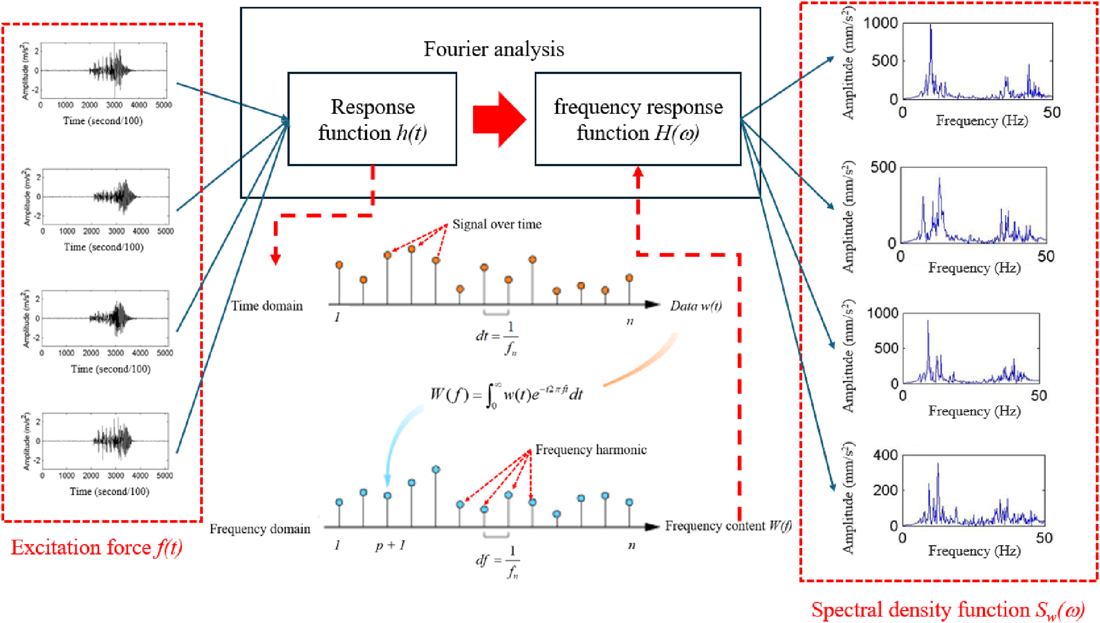
This study uses the vibration signal measured to construct the power spectral density (PSD) ¹⁴ model based on which structural changes can be assessed when damage occurs. The authors also propose the zeroth spectral moment and the first spectral moment models to predict structural changes over time. ¹⁴ The theoretical model in Figure 5 illustrates the stages of forming the theoretical models, where the laboratory vibration signal measurements are transformed using the Fourier transform method to form the vibration spectra. ⁷² Essentially, this spectral model is a conversion from the time-domain spectral model^70,71 (from measured data) to the frequency-domain spectral model. ⁷³

Figure 5.

Proposed theoretical models from data analysis.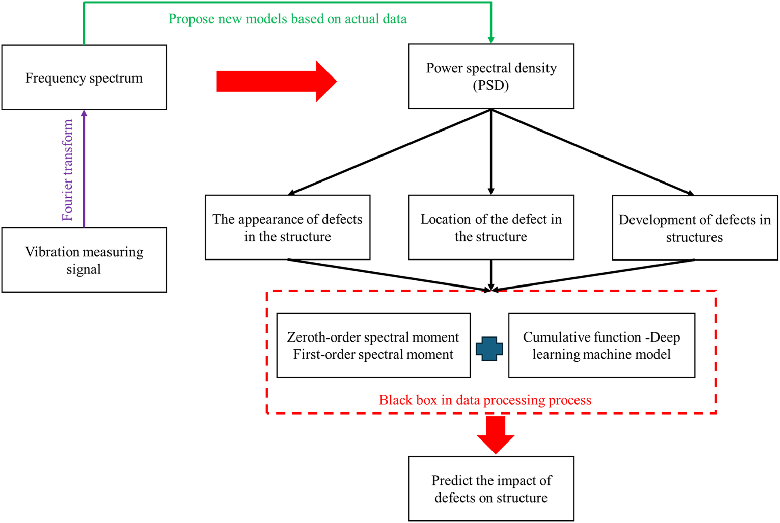

In structural dynamics analysis, the stimulating force f(t) acting on the structure and the response function h(t) are considered as the input and output of a system described in a general form as shown in Figure 6. Assume that the beam structure studied is a linear system characterized by a linear relationship between the input and output through the transfer function h(t) at time t. Thus, at time τ, the function h(τ) contains all mechanical characteristics of the system, as well as its response over time. In this case, the theory illustrates the relationship between the response and the stimulating force function, as expressed in equations (1a-b):

$w\left(t\right)=\underset{-\infty }{\overset{t}{{\displaystyle \int }}}h\left(t-\tau \right)f\left(\tau \right)d\tau$

(1a)

$w\left(\omega \right)=h\left(\omega \right)f\left(\omega \right)$

(1b)

Figure 6.

The relationship between the input and output of the linear system.

Equations (1a-b) form the core framework for analyzing structural damage using spectral moments. These equations are based on well-established research in structural health monitoring and serve as the foundation for calculating spectral moment values, which are crucial in capturing variations in the structural response caused by damage. Their application enables precise detection of changes in frequency response, a key factor in identifying damage. In this study, we extend the use of these equations by incorporating them into a novel methodology for damage identification in beam structures, particularly through the innovative application of cumulative spectral moment models, which enhances detection accuracy and reliability.

Through the Fourier transform, the frequency response function H(ω) and F(ω) in equations (2a-b) are the transformations of the response function h(t) and the force function f(t) of the original model.

$H\left(\omega \right)=\underset{-\infty }{\overset{\infty }{{\displaystyle \int }}}h\left(t\right)e^{-i\omega t}dt$

(2a)

$F\left(\omega \right)=\underset{-\infty }{\overset{\infty }{{\displaystyle \int }}}f\left(t\right)e^{-i\omega t}dt$

(2b)

In that case, the power spectral density function S _w (ω) of the responses input by w(t) of the linear system is calculated through the frequency response function W(ω), thus the power spectral density function of the output force function output S _f (ω) is as follows:

$S_w\left(\omega \right)={\left|H\left(\omega \right)\right|}^2{S}_f\left(\omega \right)$

(3)

For a single degree-of-freedom system, the frequency response function H(ω) takes the form:

$H\left(\omega \right)=\frac{1}{-{\omega }^2+2i\xi {\omega }_0\omega +{\omega }_0^2}$

(4)

Where: ω ₀ and ξ are respectively the natural frequency and the damping ratio of the system. Similarly, for multidegree-of-freedom systems, the frequency response matrix takes the form:

$\left[H\left(\omega \right)\right]=\frac{1}{-{\omega }^2\left[M\right]+i\omega \left[C\right]+\left[K\right]}={{\displaystyle \sum }}_{j=1}^n\frac{\left\{{\varphi }_j\right\}{\left\{{\varphi }_j\right\}}^T}{{\mu }_j\left[\left({\omega }_j^2-{\omega }^2\right)+2i{\xi }_j{\omega }_j\right]}$

(5)

Where [M], [C], [K], and respectively represent the mass matrix, damping matrix, stiffness matrix, and mode shapes of the system.

According to the statistical theory model, the distribution of random response values in the time domain indicates the extent of spread of the data set from the smallest to the largest values. However, in the frequency domain, the power spectral density function provides us with the distribution of energy. Therefore, the M spectral moment model (spectral moment) proposed in this study aims to investigate the energy distribution characteristics of the response signals in each frequency domain.

$M_n=\underset{-\infty }{\overset{\infty }{{\displaystyle \int }}}{\left|\omega \right|}^n{S}_w\left(\omega \right)d\omega$

(6)

In cases where the characteristics of the output signal are complex, such as in random defect diagnosis problems or multi-layered force functions, the concept of spectral moments defines the characteristic parameters in determining faults and monitoring the operational status of structures. If w(t) is the response of the displacement of the system, then by definition, the first three even-order spectral moments M₀, M₂, M₄, respectively, represent the zeroth-order spectral moment of the displacement response equation (7a), velocity equation (7b), and acceleration equation (7c). These moments are used to describe the distribution values of the extrema, the mean frequency, or the cycle of the random process. Where:

$M_0=\underset{-\infty }{\overset{\infty }{{\displaystyle \int }}}{S}_w\left(\omega \right)d\omega$

(7a)

$M_2=\underset{-\infty }{\overset{\infty }{{\displaystyle \int }}}{\omega }^2{S}_w\left(\omega \right)d\omega$

(7b)

$M_4=\underset{-\infty }{\overset{\infty }{{\displaystyle \int }}}{\omega }^4{S}_w\left(\omega \right)d\omega$

(7c)

The spectral moment is a statistical quantity that provides insights into the energy distribution of a signal across various frequency ranges. Each order of the spectral moment holds distinct physical meaning in describing the characteristics of the vibration response:

• Zeroth-order spectral moment (M ₀ ) represents the total energy of the signal. It is a key indicator of the cumulative energy during the vibration process.

• Second-order spectral moment (M ₂ ) reflects the average frequency of the spectrum, showing the central tendency of the frequency distribution. This helps to evaluate how energy is distributed around the central frequency.

• Fourth-order spectral moment (M ₄ ) provides information about the spread of energy around the central frequency, indicating the variance or dispersion of energy across the spectrum. By calculating these spectral moments, we can identify changes in the energy distribution of the signal, which can be used to detect structural damage. This is particularly useful in identifying early or subtle changes in structural conditions that traditional methods may overlook.

For higher-order spectral moments, the concept of central moments is proposed to examine the shape of the spectrum around the central frequency $\overline{\omega }$

$s{m}_{\left(k\right)}=\frac{1}{S{M}_{\left(0\right)}}\underset{-\infty }{\overset{\infty }{{\displaystyle \int }}}{\left(\omega -\overline{\omega }\right)}^k{S}_{w}d\omega$

(8)

Equation (8) introduces the concept of central spectral moments, which are used to examine the shape of the spectrum around its central frequency. These moments are especially important for analyzing non-linear or time-varying signals, where the frequency components of the signal may not remain stable over time. Specifically, the central spectral moment is computed by subtracting the central frequency from each frequency component and raising this difference to a specified power (depending on the moment order). This process allows central moments to capture subtle changes in the frequency distribution, such as shifts or deformations in the signal caused by damage. By using central moments, we can detect more nuanced variations in the dynamic response of the structure, providing a deeper understanding of its condition. This approach enhances the ability to assess and monitor structural health more effectively.

If the acquired signal consists of discrete values, the spectral moments in the frequency domain can be determined by the formulas equations (9), and (10):

$M_{\left(n\right)}=\frac{1}{N}{{{\displaystyle \sum }}_{i=0}^{\left(N-1\right)}{S}_w\left(i\right)\left(\frac{i}{N\mathrm{\Delta }t}\right)}^n$

(9)

$s{m}_{\left(k\right)}=\frac{1}{S{M}_{\left(0\right)}N}{{{\displaystyle \sum }}_{i=0}^{\left(N-1\right)}{S}_w\left(i\right)\left(\frac{i}{N\mathrm{\Delta }t}-s{m}_{\left(1\right)}\right)}^k;k>2$

(10)

In this case, N is half the length of the discrete signal spectrum, where N = T/(2Δt). Here, Δt is the time interval between samples and T is the duration of the sampling.

Spectral moment of vibration for multi-degree-of-freedom systems

Considering the case of a continuous linear system, assume that it is in a stable state undergoing random excitation f(s,t) at position s of the system as shown in Figure 7. The coordinates r and s belong to the defined domain |R |. Similarly to the response matrix of multidegree-of-freedom systems, the dynamic properties of continuous systems can be described through the unit response function h(r,s,t) or the frequency response function H(r,s,ω). The function h(r,s,t) represents the response (displacement) of the structure at position r when subjected to a unit load at position s of the system at the initial time t = 0. Initially, the system is assumed to be at rest. The frequency response function H(r,s,ω) is the harmonic response of the structure at position r when subjected to a unit harmonic excitation with frequency ω at position s.

Figure 7.

Response of the continuous system at position r when subjected to excitation at position s.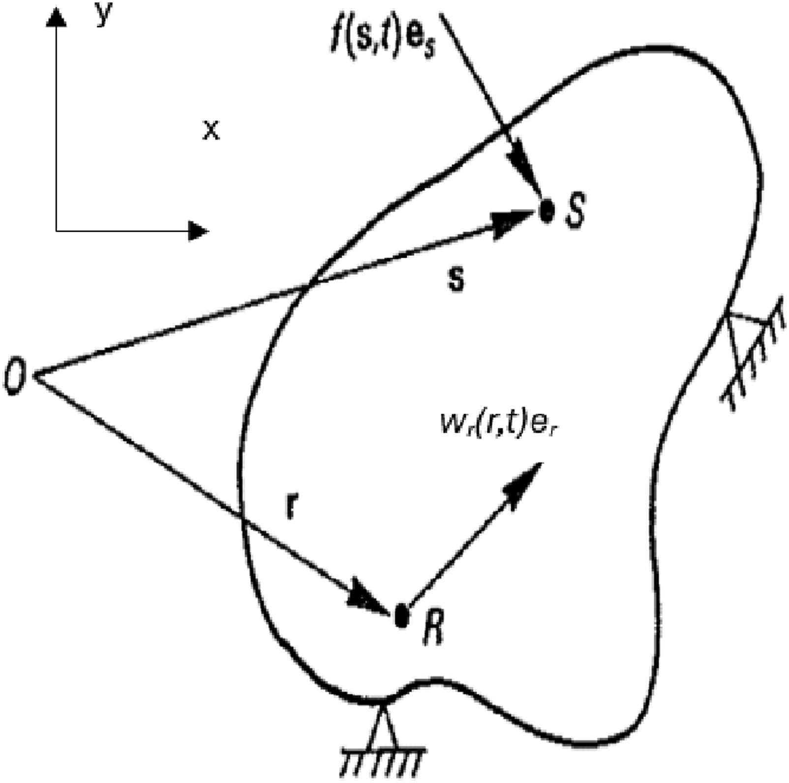

The frequency response function and the impulse response function are a pair of Fourier transforms with each other:

$H\left(r,s,\omega \right)=\underset{-\infty }{\overset{\infty }{{\displaystyle \int }}}h\left(r,s,t\right)e^{-i\omega t}dth\left(r,s,t\right)=\frac{1}{2\pi }\underset{-\infty }{\overset{\infty }{{\displaystyle \int }}}H\left(r,s,\omega \right)e^{i\omega t}d\omega$

(11)

When f(s,t) is the sole excitation source with S _f (s,ω) being the spectral density of the force function, the response value and the power spectral density function of the response at position r have the following forms:

$w_r\left(r,t\right)=\underset{0}{\overset{t}{{\displaystyle \int }}}\underset{R}{{\displaystyle \int }}h\left(r,s,t-\tau \right)f\left(s,\tau \right)d\tau ds$

(12)

$S_w\left(r,\omega \right)=H^{*}\left(r,s,\omega \right)H\left(r,s,\omega \right)S_f\left(s,\omega \right)$

(13)

Considering a continuous system with mass m and damping c subjected to an external force, the equation of motion takes the form:

$m{\ddot{w}}_r+c{\dot{w}}_r+L\left(w_r\right)=f\left(s,t\right)$

(14)

The eigenfunction $\varphi \left(r\right)$ of the system is the solution of the expression:

$m{\omega }_j^2{\varphi }_j\left(r\right)=L\left[{\varphi }_j\left(r\right)\right]$

(15)

And the orthogonal relationship must be satisfied:

$\underset{R}{{\displaystyle \int }}{\varphi }_i\left(r\right){\varphi }_j\left(r\right)dr=R{\delta }_{ij}$

(16a)

$\text{Put}:\underset{R}{{\displaystyle \int }}m\left(r\right){\varphi }_i\left(r\right){\varphi }_j\left(r\right)dr=m_j{\delta }_{ij}$

(16b)

$\underset{R}{{\displaystyle \int }}c\left(r\right){\varphi }_i\left(r\right){\varphi }_j\left(r\right)dr=c_j{\delta }_{ij}=2{\mu }_j{\omega }_j{\xi }_j{\delta }_{ij}$

(16c)

In there: $m_j,{\omega }_j,{\xi }_j$ respectively represent the mass ratio, natural frequency, and damping ratio of the ith mode of vibration. Assuming that the solution of the differential equation can be found in the form:

$w_r\left(r,t\right)={{\displaystyle \sum }}_{j=1}^{\infty }{\varphi }_j\left(r\right)w_j\left(t\right)$

(17)

With the solution equation (16), substituting into the differential equation (17), multiplying both sides by the function of mode shape (r), and integrating throughout the spatial domain of the system, we obtain the vibration equation for each individual mode of vibration as follows:

${\ddot{w}}_j+2{\omega }_j{\xi }_j{\dot{w}}_j+{\omega }_j^2{w}_j=\frac{1}{m_i}\underset{R}{\overset{\int }{{\displaystyle \int }}}{\varphi }_j\left(r\right)f(r)$

(18a)

$c=2m_j{\omega }_j{\xi }_j$

(18b)

Assume that the force function f(s,t) takes the form of an arbitrary function at any position s.

$f\left(s,t\right)=f\left(t\right)\delta \left(r-s\right)$

(19)

Where δ is the Dirac delta function. Equation (18a) will become:

${\ddot{w}}_j+2{\omega }_j{\xi }_j{\dot{w}}_j+{\omega }_j^2{w}_j=\frac{f\left(t\right)}{m_j}{\varphi }_j\left(s\right)=f_j\left(t\right)$

(20)

We can see that the continuous system is a collection of single-degree-of-freedom systems with individual natural frequencies. The solution of equation (20) can be written in the following form:

$w_j\left(t\right)=\underset{-\infty }{\overset{\infty }{{\displaystyle \int }}}{H}_j\left(\omega \right)F\left(\omega \right)e^{i\omega t}d\omega$

(21a)

$\text{with}\hspace{0.17em}{H}_j\left(\omega \right)=\frac{1}{\left(-{\omega }^2+2i{\xi }_j{\omega }_j\omega +{\omega }_j^2\right)}$

(21b)

From the frequency response function at each mode, we obtain the frequency response function of the system:

$H\left(r,s,\omega \right)={{\displaystyle \sum }}_{j=1}^{\infty }{\varphi }_j\left(r\right)H_j\left(\omega \right){\varphi }_j\left(s\right)$

(22)

From equations (21a) and (22), the power spectral density function of the system is determined by the following: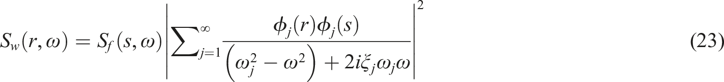

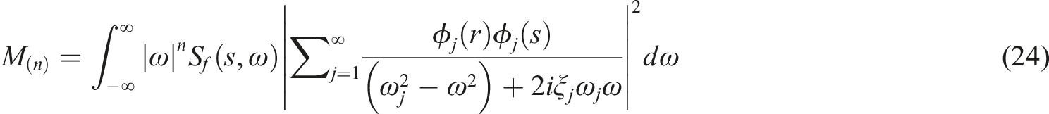
$S_w\left(r,\omega \right)=S_f\left(s,\omega \right){\left|{{\displaystyle \sum }}_{j=1}^{\infty }\frac{{\varphi }_j\left(r\right){\varphi }_j\left(s\right)}{\left({\omega }_j^2-{\omega }^2\right)+2i{\xi }_j{\omega }_j\omega }\right|}^2$

(23)

In that case, the SM spectral moment of the response is calculated as follows:

$M_{\left(n\right)}=\underset{-\infty }{\overset{\infty }{{\displaystyle \int }}}|\omega {|}^n{S}_f\left(s,\omega \right){\left|{{\displaystyle \sum }}_{j=1}^{\infty }\frac{{\varphi }_j\left(r\right){\varphi }_j\left(s\right)}{\left({\omega }_j^2-{\omega }^2\right)+2i{\xi }_j{\omega }_j\omega }\right|}^{2}d\omega$

(24)

On the basis of equation (24), although the spectral moment is a non-state property of random vibration, this parameter depends on the state parameters of the random response such as natural frequency, damping, and mode shape. However, unlike individual response parameters that provide local information at each specific frequency, spectral moments are global data that contain much information about a range of frequencies. Spectral moments can be understood as the sum of all harmonic frequencies with appropriate weights. Defects that appear at different locations will affect the specific frequencies of the structure. The general changes at these frequencies through the spectral moment values can provide information about defects within the structure.

Parameters influencing the effectiveness of zeroth-order spectral moment (M₀) in damage detection and localization

The effectiveness of the zeroth-order spectral moment (M₀) in detecting and localizing structural damage is influenced by several critical parameters. Sensor placement and density play a pivotal role, as strategically positioned sensors near regions prone to high stress or potential damage enhance the sensitivity and precision of energy redistribution analysis. Insufficient sensor coverage may lead to undetected localized damage. Another key factor is the signal-to-noise ratio (SNR), as high-quality vibration signals ensure that subtle energy shifts caused by damage are not obscured by environmental noise. Preprocessing techniques, such as noise filtering, are essential to improve data reliability.

Additionally, the frequency resolution of the analysis significantly impacts M₀’s ability to detect damage. Higher frequency resolution enables more precise identification of energy shifts across specific zones, which can be achieved through appropriate sampling rates and windowing techniques during signal acquisition. The structural and material properties—such as stiffness, mass distribution, and damping—also influence the energy distribution within the frequency domain. Accurately modeling these properties ensures that M₀ analysis effectively reflects structural responses.

The loading conditions are another critical parameter. Dynamic loads, such as those caused by moving vehicles or wind forces, introduce specific frequency components that interact with the structural properties and impact the vibration response. Representative loading conditions during experimental or field analysis improve the applicability of M₀ in real-world scenarios. Furthermore, the characteristics of the damage—including its size, location, and severity—affect the extent to which it alters the energy distribution. While severe or extensive damage produces clear shifts in spectral moments, minor or early-stage damage may require enhancements through cumulative spectral moment models or higher-order moments to achieve accurate detection.

Finally, integrating cumulative spectral moment models with M₀ analysis provides a robust framework for tracking damage progression over time. By aggregating changes in M₀ values across multiple measurements, this approach improves sensitivity and enables precise identification of subtle or progressive damage. Collectively, these parameters underscore the adaptability and effectiveness of M₀ in structural health monitoring when properly optimized for specific applications.

Building the cumulative distribution function model

The probability distribution function of a set of data is represented by the curve of the Gaussian distribution function (PDF - Probability distribution functions) and is expressed as equations (25a-b)

$P\left(X\ge x\right)=\frac{1}{\sqrt{2\pi \sigma }}{{\displaystyle \int }}_x^{\infty }\mathit{exp}\left\{-\frac{1}{2}{\left(\frac{x-\overline{x}}{\sigma }\right)}^2\right\}dx$

(25a)

$P\left(X\ge x\right)=1-\frac{1}{\sqrt{2\pi \sigma }}\underset{-\infty }{\overset{x}{{\displaystyle \int }}}\mathit{exp}\left\{-\frac{1}{2}{\left(\frac{x-\overline{x}}{\sigma }\right)}^2\right\}dx$

(25b)

Equations (25a-b) provide the likelihood of a random variable taking a particular value within a given range. It shows how the values of the variable are distributed around the mean. If we normalize the quantity $\frac{x-\overline{x}}{\sigma }=z$ , then z is called the standardized variable such that the distribution of the z values falls within the range of N(0,1). In this case, equations (25a-b) is modified to equations (26a-b)

$P\left(X\ge x\right)=\frac{1}{\sqrt{2\pi \sigma }}{{\displaystyle \int }}_x^{\infty }\mathit{exp}\left\{-\frac{1}{2}{z}^2\right\}dx=\Phi \left(z\right)$

(26a)

$P\left(X\ge x\right)=1-\frac{1}{\sqrt{2\pi \sigma }}\underset{-\infty }{\overset{x}{{\displaystyle \int }}}\mathit{exp}\left\{-\frac{1}{2}{z}^2\right\}dx=1-\Phi \left(z\right)$

(26b)

Equations (26a-b) give the cumulative probability that the random variable is less than or equal to a certain value. It represents the total probability that the variable falls within or below a certain threshold. In that case, the function Φ(z) is called the cumulative distribution function (CDF) for N(0,1). The term N(0,1) refers to the standard normal distribution, which has a mean of 0 and a standard deviation of 1. In this context, N(0,1) is used to standardize the variable, meaning that the random variable has been scaled and shifted so that it fits the standard normal distribution. Standardization simplifies the process of calculating probabilities using the CDF, as any normally distributed variable can be transformed to N(0,1) through this process.

The CDF is less explored than the Gaussian distribution function; however, the representation of the distribution values will become more apparent. The PDF as in equations (25a-b) describes the probability density of a random variable at any specific point, while the CDF as shown in equations (26a-b) represents the integral of the PDF up to a certain point, capturing the cumulative probability that the variable is below a given value. In the context of this study, the CDF plays a critical role in evaluating structural damage. By analyzing the CDF of the measured vibration signals, we can observe how the data distribution changes over time, which may indicate the development or progression of structural defects. The CDF provides a more intuitive and comprehensive view of the probability distribution compared to the PDF alone, especially when assessing the cumulative impact of damage on a structure. Figure 8 shows a segment of the real-time signal over time, and the data set of this segment is represented by two parameters (PDF) and (CDF) as shown in Figure 9.

Figure 8.

An actual signal measured in the laboratory.

Figure 9.

Distribution rules between (PDF) and (CDF) of the signal from Figure 8.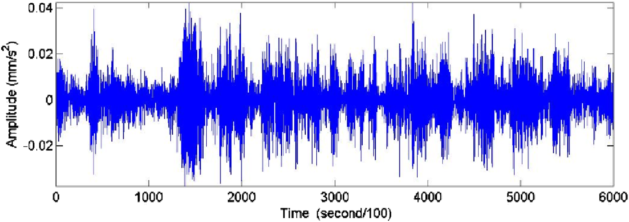

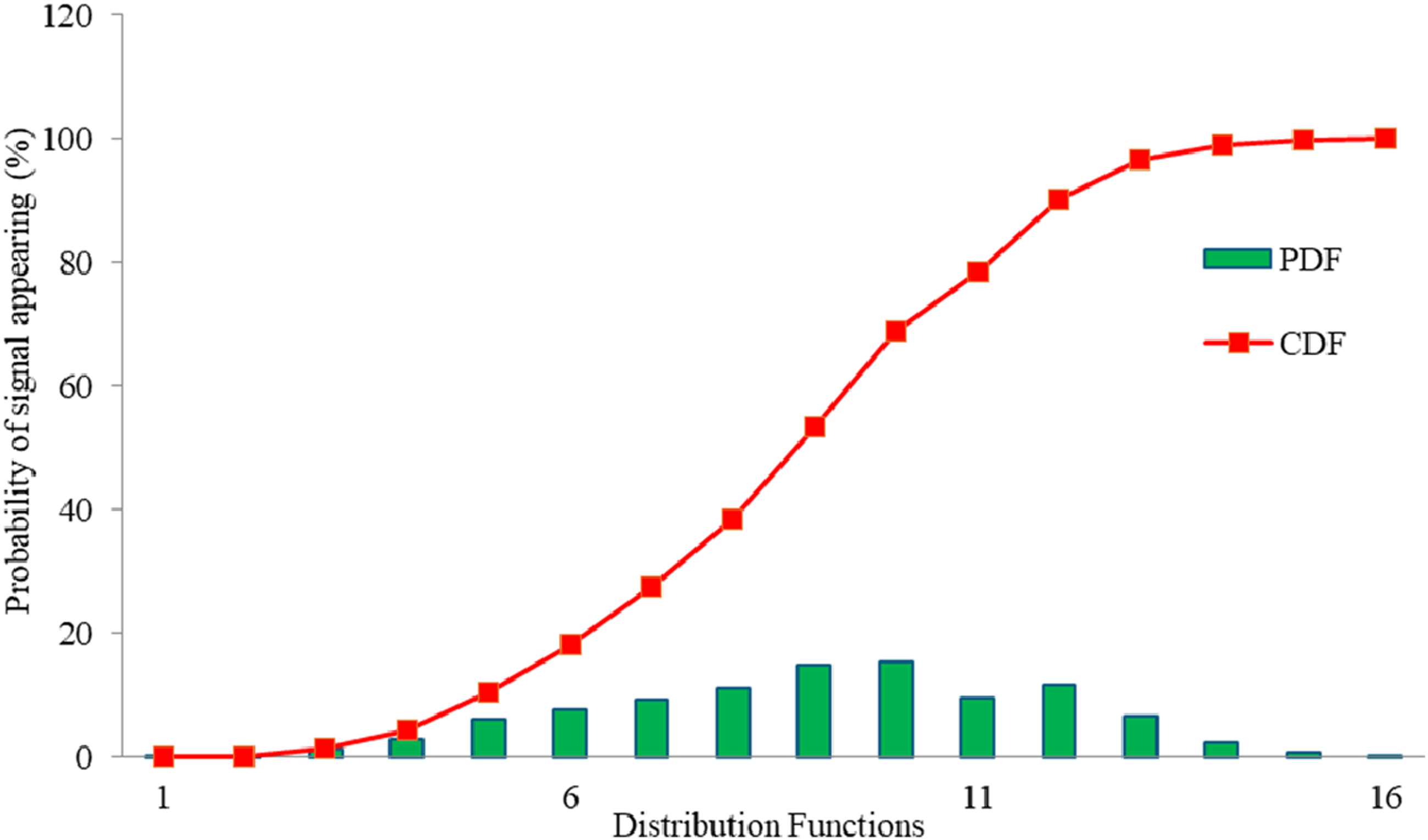
In Figure 9, it is evident that the distribution law obtained from the CDF of the signal over time is much better than the PDF model. From this observation, the authors propose to use CDF features when assessing structural changes over time using the data measurement model.

Structural dynamics model of beams

A beam structure is a model with dimensions where the length of the structure is much greater than its cross-sectional dimension. This study adopted a steel beam supported with a simple frame as shown in Figure 10.

Figure 10.

Beam model.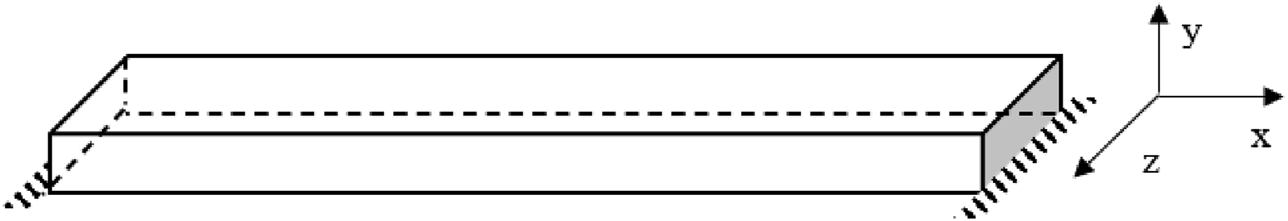

It is assumed that the beam behaves linearly during all load states so that according to the superposition principle, structural quantities such as displacement, deformation, or stress are considered as combinations of individual load cases. The effects of traffic loads on bridges can be separated into basic forms, such as axial, bending, torsion, and combined bending-torsion.

Basic vibration modes

Assume that the beam has a very small damping coefficient that can be neglected in this study.

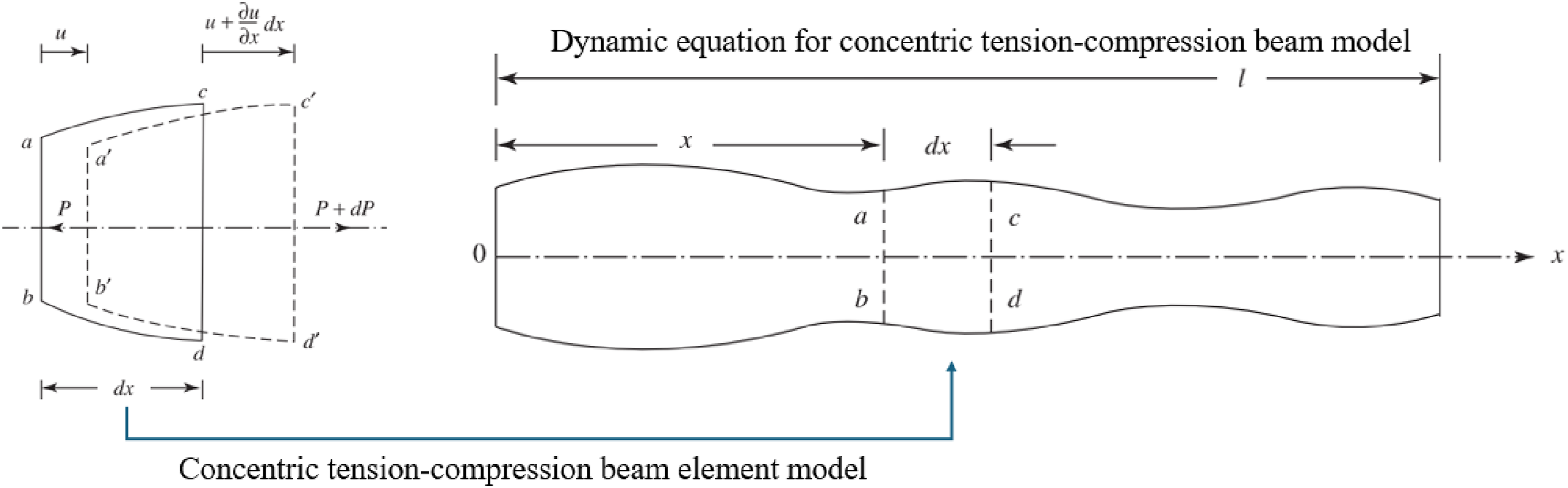
Longitudinal vibration of the beam structure under the action of axial force

On the basis of equation (27), where equation (27a) represents the dynamic equation of the beam structure subjected to axial tension and compression, and the natural frequency of this structural model is expressed as equation (27b), using the method of separation of variables from equation (27a), the solution of the equation is represented as equation (27c). Through equation (27c), we obtain an equation where we have the basic modes of vibration of the beam structure, as shown in Figure 11.

$\text{Differential}\hspace{0.17em}\text{equation}:EA\frac{{\partial }^{2}u}{\partial z^2}\left(x,t\right)+f\left(x,t\right)=\rho A\frac{{\partial }^{2}u}{\partial t^2}\left(x,t\right)$

(27a)

$\text{Fundamental}\hspace{0.17em}\text{natural}\hspace{0.17em}\text{frequency}:{\omega }_{\mathit{Ln}}=\frac{n\pi }{l}\sqrt{\frac{E}{\rho }}$

(27b)

$\text{Specific}\hspace{0.17em}\text{function}:U_n\left(x\right)={\varphi }_{\mathit{Ln}}\left(x\right)=C_n\hspace{0.17em}\mathit{cos}\frac{n\pi x}{l}$

(27c)

With u as the longitudinal displacement along the x-axis, l as the length of the beam, E as the modulus of elasticity, ρ as the mass density of the beam, and A as the cross-sectional area.

Figure 11.

Axial vibration of the bar.

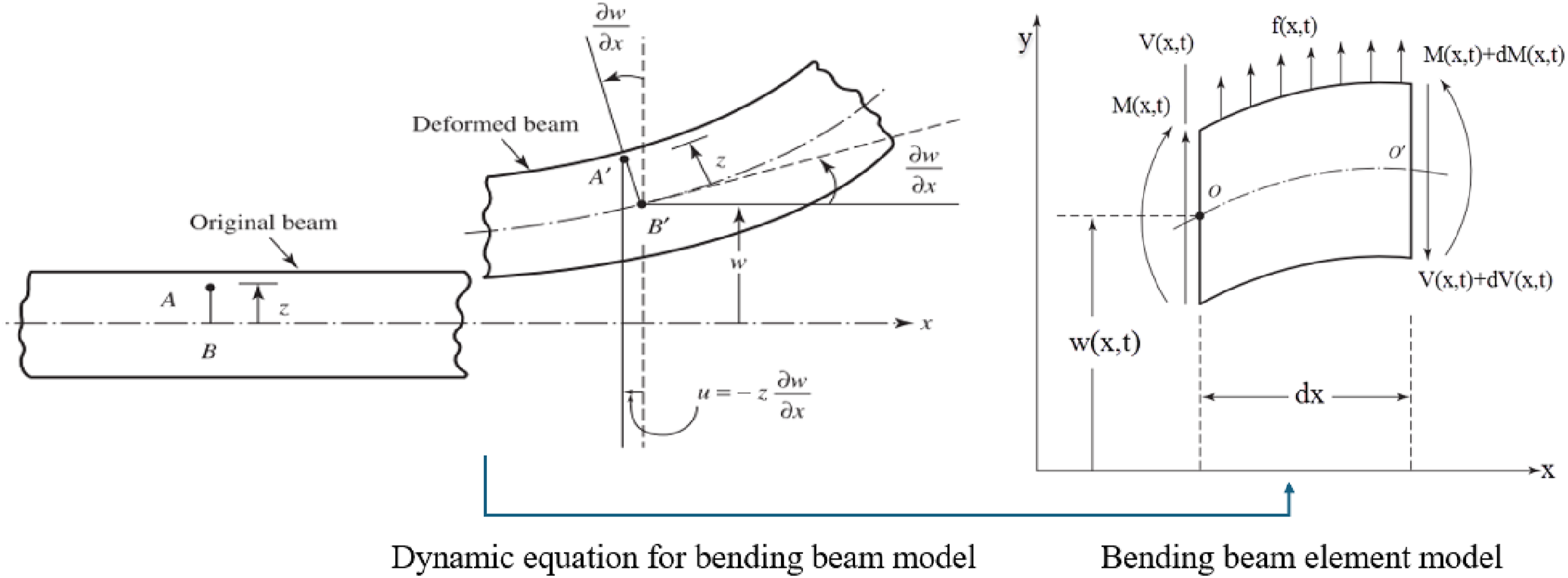
The bending vibration of the beam structure under the effect of forced force

Similarly to the longitudinal vibration model of the beam shown in Figure 11, the bending vibration model of the beam under the action of a forced load is depicted in Figure 12

$\text{Differential}\hspace{0.17em}\text{equation}:E{J}_z\frac{{\partial }^{2}w}{\partial z^2}\left(x,t\right)+f\left(x,t\right)=\rho A\frac{{\partial }^{2}w}{\partial t^2}\left(x,t\right)$

(28a)

$\text{Fundamental}\hspace{0.17em}\text{natural}\hspace{0.17em}\text{frequency}:{\omega }_{Bn}={\left(n\pi l\right)}^2\sqrt{\frac{E{J}_z}{\rho A}}$

(28b)

$\text{Specific}\hspace{0.17em}\text{function}:W_n\left(x\right)={\varphi }_{Bn}\left(x\right)=B_n\hspace{0.17em}\mathit{sin}\frac{n\pi x}{l}$

(28c)

where w is the displacement in the y direction, J _z is the cross-sectional moment of inertia on the z axis.

Figure 12.

Bending vibration of the beam structure.

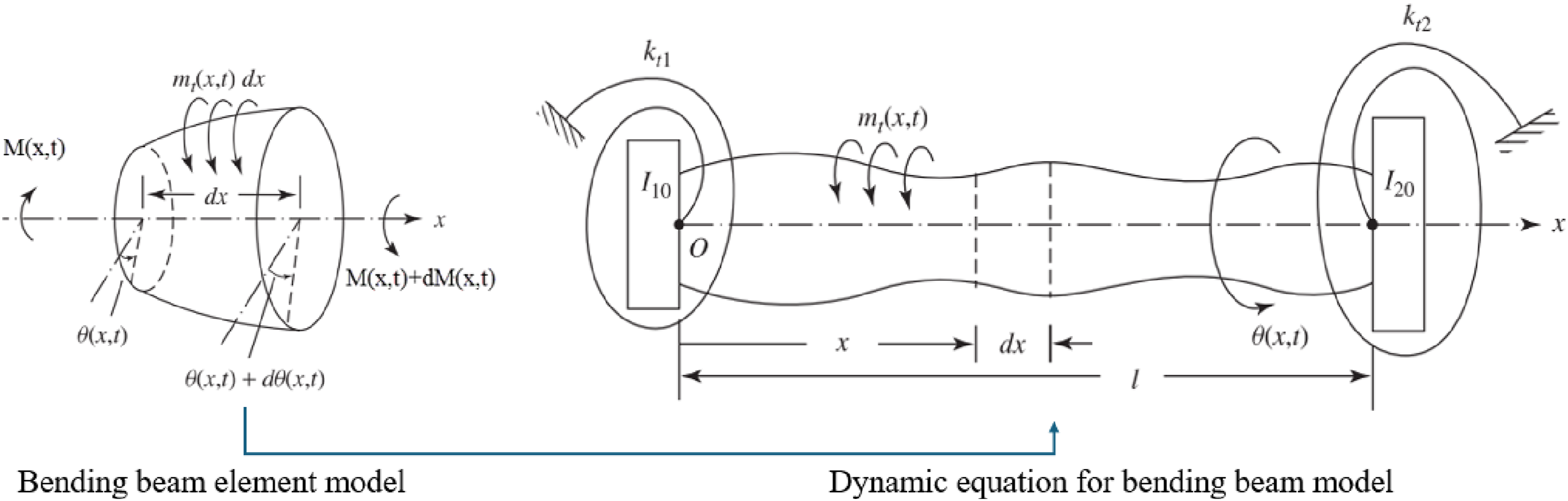
Torsional vibration of beam structure under the effect of forced force

$\text{Differential}\hspace{0.17em}\text{equation}:G{J}_x\frac{{\partial }^2\theta }{\partial z^2}\left(x,t\right)+f\left(z,t\right)=J_0\frac{{\partial }^2\theta }{\partial t^2}\left(x,t\right)$

(29a)

$\text{Fundamental}\hspace{0.17em}\text{natural}\hspace{0.17em}\text{frequency}:{\omega }_{Tn}=\frac{n\pi }{l}\sqrt{\frac{G{J}_x}{J_0}}$

(29b)

$\text{Specific}\hspace{0.17em}\text{function}:{\theta }_n\left(x\right)={\varphi }_{Tn}\left(x\right)=T_n\hspace{0.17em}\mathit{cos}\frac{n\pi x}{l}$

(29c)

Where θ is the rotation angle of the cross section about the x-axis, G is the shear elastic modulus, J ₀ is the mass moment of inertia per unit length. J _x the moment of inertia of the section on the x axis, as shown in Figure 13.

Figure 13.

Torsional vibration of the bar.

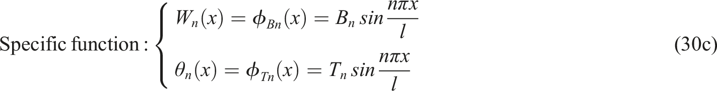
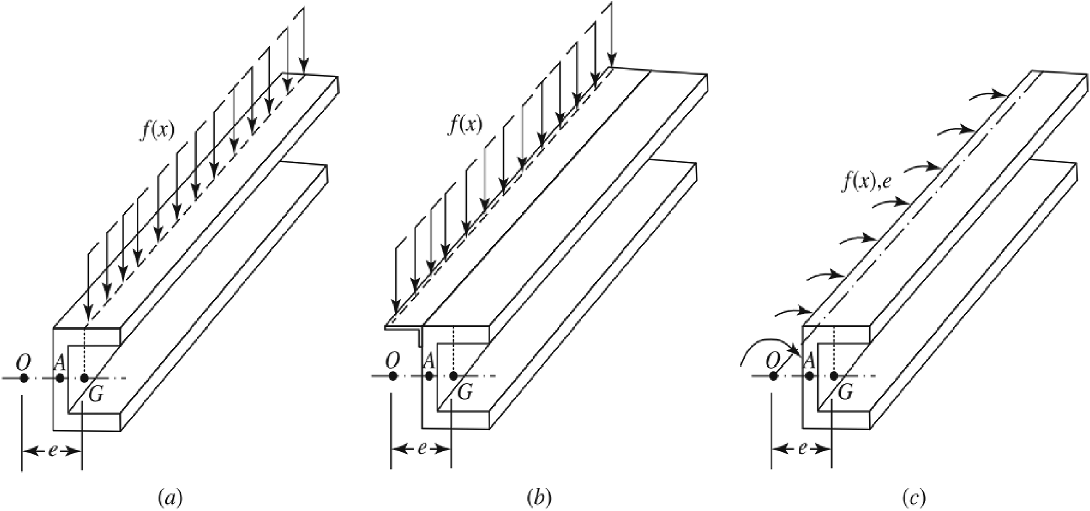
Simultaneous bending-torsional vibrations of the beam structure under the effect of a forced load

$\text{Differential}\hspace{0.17em}\text{equation}:\{\begin{array}{l}E{J}_z\frac{{\partial }^{2}w}{\partial z^2}\left(x,t\right)+f\left(x,t\right)=\rho A\frac{{\partial }^2\left(w-e\theta \right)}{\partial t^2}\left(x,t\right)\\ G{J}_x\frac{{\partial }^2\theta }{\partial z^2}\left(x,t\right)-{EJ}_w\frac{{\partial }^4\theta }{\partial z^4}\left(x,t\right)+f\left(x,t\right)e=\rho Ae\frac{{\partial }^2\left(w-e\theta \right)}{\partial t^2}\left(x,t\right)+\rho J_G\frac{{\partial }^2\theta }{\partial t^2}\left(x,t\right)\end{array}$

(30a)

$\text{Fundamental}\hspace{0.17em}\text{natural}\hspace{0.17em}\text{frequency}:{\omega }_{BTn}^2=\frac{\left({\omega }_{Tn}^2+{\omega }_{Bn}^2\right)\pm \sqrt{{\left({\omega }_{Tn}^2-{\omega }_{Bn}^2\right)}^2+4\lambda {\omega }_{Tn}^2{\omega }_{Bn}^2}}{2\left(1-\lambda \right)}$

(30b)

$\text{Specific}\hspace{0.17em}\text{function}:\{\begin{array}{l}{W}_n\left(x\right)={\varphi }_{Bn}\left(x\right)=B_n\hspace{0.17em}\mathit{sin}\frac{n\pi x}{l}\\ {\theta }_n\left(x\right)={\varphi }_{Tn}\left(x\right)=T_n\hspace{0.17em}\mathit{sin}\frac{n\pi x}{l}\end{array}$

(30c)

In which

${\omega }_{Bn}^2=\frac{E{J}_x{n}^4{\pi }^4}{l^4\rho A};\hspace{0.17em}{\omega }_{Tn}^2=\frac{G{J}_z{n}^2{\pi }^2{l}^2+E{J}_w{n}^4{\pi }^4}{l^4\rho \left(J_G+A{e}^2\right)};\hspace{0.17em}\lambda =\frac{A{e}^2}{J_G+A{e}^2}$

(30d)

In that case, where e is the distance from the center of shear to the symmetry axis of the beam shown in Figure 14, J _G is the monopole moment about the center of the cross section and J _w is the inertia sectional polar moment.

Figure 14.

Types of bar bearing. (a) Vertical force at center of gravity, (b) longitudinal force at sliding center, (c) moment at sliding center.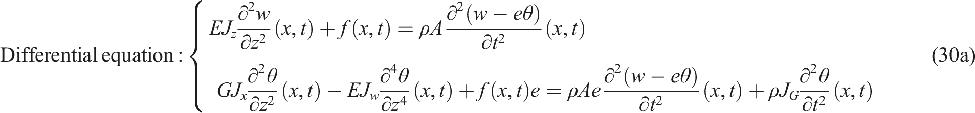

Forced vibration

The form of vibration at each natural frequency is commonly referred to as the mode shape function ϕ _n (z) of the system. The vibration equation for each mode shape of the structure with damping takes the form of as shown in equation (31):

${\ddot{q}}_j+2{\omega }_j{\xi }_j{\dot{q}}_j+{\omega }_j^2{q}_j=\underset{0}{\overset{l}{{\displaystyle \int }}}f\left(x,t\right){\varphi }_j\left(x\right)dx=F_j\left(t\right)$

(31)

In which: q _j is the standard coordinate of the j-th, f(x,t) is the active force per unit length of the bar, ω _j and ξ _j are the natural frequency and damping coefficient of the function of the j-th form, respectively, f _j (t) are the standard specific load of the function of the j-th shape in the generalized coordinate system.

Harmonic force function

If the behavior of the bridge structure is caused by the application of a harmonic forcing force f _j (t) = F _j sinωt then q(t) in equation (31) will be a function of the frequency of that forcing force, and the amplitude depends on the relationship between the forcing frequency and the natural frequency of the system.

$q_j=q_{0j}\hspace{0.17em}\mathit{sin}\left(\omega t-\phi \right)$

(32a)

$q_{0j}=F_j{H}_j\left(\omega \right)=\frac{F_j/k}{\sqrt{{\left(1-{\left(\omega /{\omega }_j\right)}^2\right)}^2+{\left(2{\xi }_j\omega /{\omega }_j\right)}^2}}$

(32b)

$\mathit{tan}\hspace{0.17em}\phi =\frac{2\xi \frac{\omega }{{\omega }_j}}{1-{\left(\frac{\omega }{{\omega }_j}\right)}^2}$

(32c)

In which q₀ is the vibration amplitude, H is the transfer function, and φ is the phase shift angle. We denote $\delta Q$ as the amplification factor of the vibration relative to the static displacement:

$\delta Q=\frac{q_{0}k}{f_0}=\frac{1}{\sqrt{{\left(1-{\left(\omega /{\omega }_j\right)}^2\right)}^2+{\left(2{\xi }_j\omega /{\omega }_j\right)}^2}}$

(33)

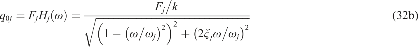
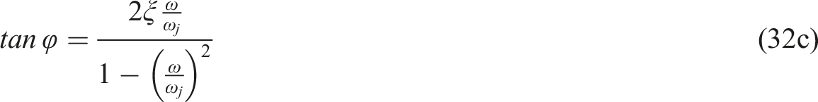
The phenomenon of significantly increased amplitude occurs at frequencies of forced vibration that coincide or are close to the natural frequencies, known as the resonance phenomenon. To ensure safety, the design process requires designing such that the natural frequencies of the components, especially the critical ones, do not coincide with the frequency of the force induced by the flow of traffic.

Random force function

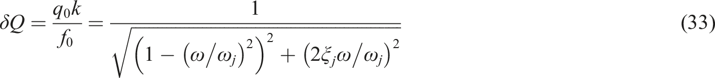
Moving objects on the bridge generate forces that cause the bridge to oscillate. The frequency of vibration depends on various factors such as the roughness of the bridge surface, the speed of the vehicle, or the inertial forces of the passing vehicles. In this case, the solution of equation (31) takes the following form after equation (34):

$q_j\left(t\right)=\frac{1}{{\omega }_{dj}}\underset{0}{\overset{l}{{\displaystyle \int }}}{\varphi }_j\left(x\right)\left[{{\displaystyle \int }}_o^t{e}^{-\xi {\omega }_j\left(t-\tau \right)}f\left(x,t\right)\mathit{sin}\hspace{0.17em}{\omega }_{dj}\left(t-\tau \right)d\tau \right]dz$

(34a)

$\text{with}\hspace{0.17em}\text{frequency}\hspace{0.17em}\text{damping}\hspace{0.17em}{\omega }_{dj}={\omega }_j\sqrt{1-{\xi }^2}$

(35)

Then, the vibrations of the mechanical system have the form:

$w\left(x,t\right)={{\displaystyle \sum }}_{j=1}^{\infty }{\varphi }_j\left(x\right)q_j\left(t\right)={{\displaystyle \sum }}_{j=1}^{\infty }\frac{{\varphi }_j\left(x\right)}{{\omega }_{dj}}\underset{0}{\overset{l}{{\displaystyle \int }}}{\varphi }_j\left(x\right)\left[{{\displaystyle \int }}_o^t{e}^{-\xi {\omega }_j\left(t-\tau \right)}f\left(x,t\right)\mathit{sin}\hspace{0.17em}{\omega }_{dj}\left(t-\tau \right)d\tau \right]dx$

(36)

In the simple case, passing vehicles create harmonic vibrations with n different frequencies ω _k , (k = 1,…,n). According to the solution from equation (31), the vibration equation of the structure takes the form:

$w\left(x,t\right)={{\displaystyle \sum }}_{j=1}^{\infty }{\varphi }_j\left(x\right)q_j\left(t\right)={{\displaystyle \sum }}_{j=1}^{\infty }{{\displaystyle \sum }}_{k=1}^n{\varphi }_j\left(x\right)F_{jk}{H}_j\left({\omega }_k\right)\mathit{sin}\hspace{0.17em}{\omega }_{k}t$

(37)

Experimental model

The experimental model in the study is presented in Figure 15. The research focuses on changing two main issues: (1) altering specific damages in the structure by creating damages and changing these damages during the experimental process and (2) changing the loading conditions on the experimental beaml.

Figure 15.

Experimental model of moving load on steel beam.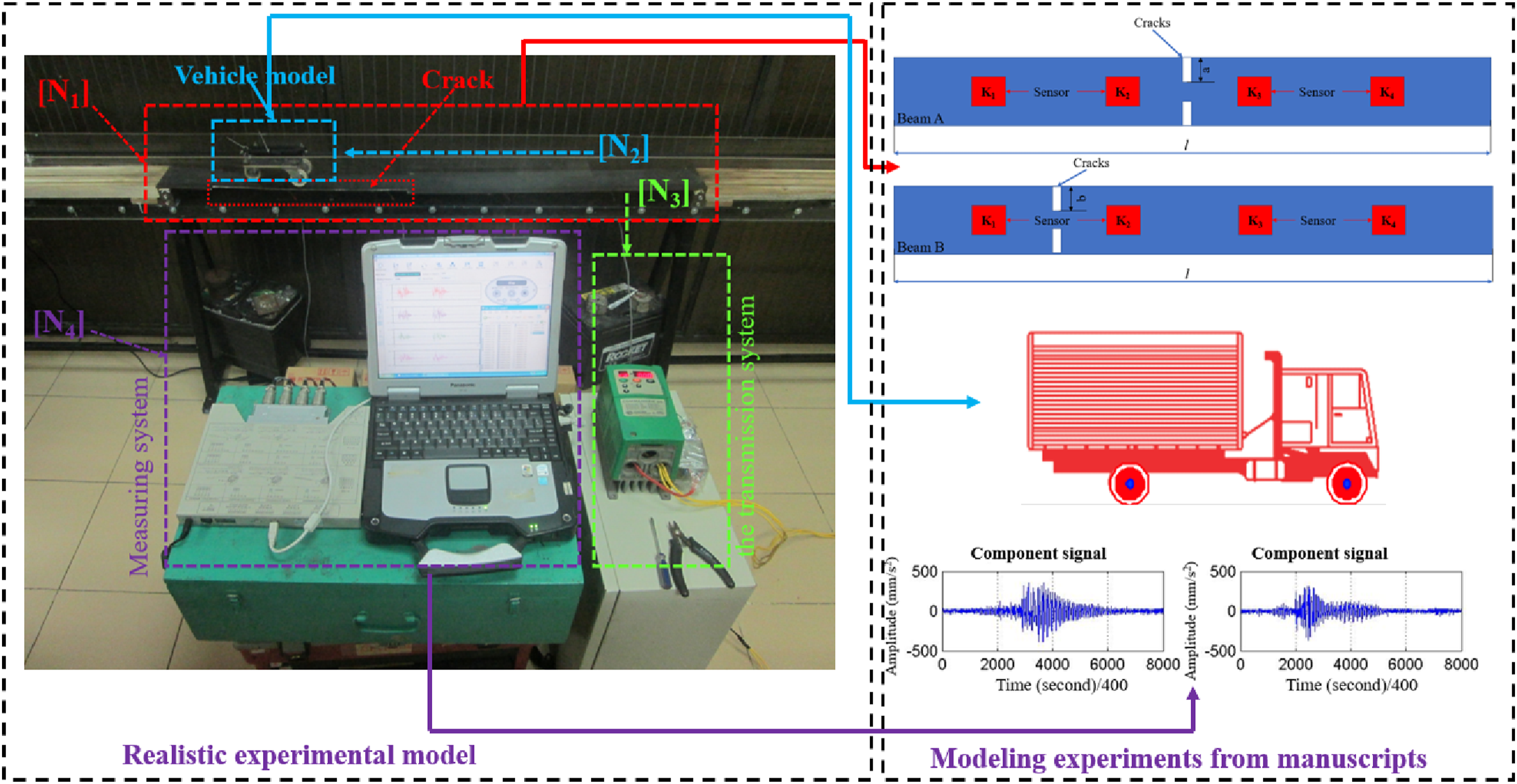

The test consists of the following main groups: structural model described by the beam structure (N1); moving load on the beam structure (N2); transmission system (N3) to assist the load moving on the structure with the ability to change the load on the structure, including the frequency converter (to change the frequency of the forced load) and motor (to change the movement speed); and measurement sensor system (N4) directly installed on the structure to collect measured data. The overall experimental model is depicted in Figure 15.

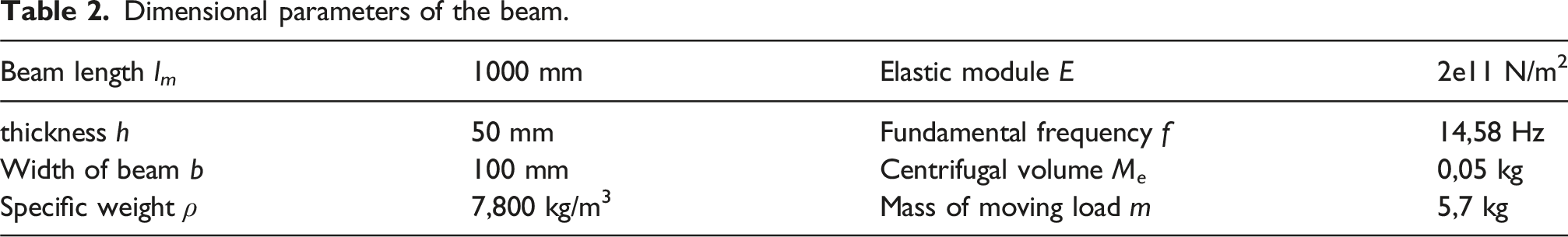
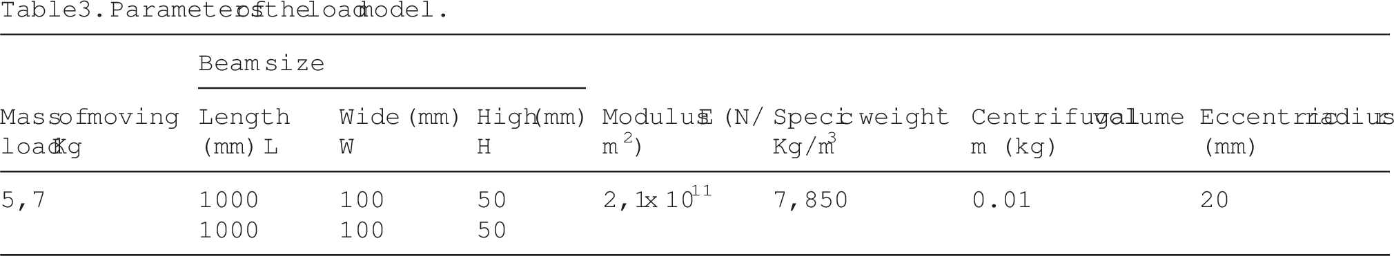
In this setup:

- Beam model [N1]: Steel beams that have or do not have defects are used. The defect posistions including (1) underneath the beam and (2) on the side of the beam.

- The beam is placed on two support pads and a rubber pad to support and absorb shock during the loading process. The parameters of all the beams [N1] are shown in Table 2.

- Moving load [N2]: The velocity of the moving load in this study is controlled through the transmission system [T3] using non-stretch cables. The parameters of the mobile load model are presented in Table 3. An eccentric block is added to the load model to generate harmonic forces Ω_i. This force can vary in rotational speed, allowing the experimental model to generate varying forces with different magnitudes and excitation frequencies.

- Drive system for loading [N3]: This system consists of a three-phase motor, a belt drive, and force control through a variable frequency drive. The purpose of the system is to transmit motion to the load, allowing it to move on the beam at different speeds.

- Measurement system [N4]: This system comprises a vibration acceleration measurement system with four sensors: VT1, VT2, VT3, VT4. They are evenly distributed along the beam, with sensor VT1 near the left support, VT2 and VT3 in the middle of the beam, and VT4 near the right support.

- The vibration measurements in this study were conducted using a high precision vibration accelerometer sensor (SENSR) with the instrument model SENSR GP 1P. The sensor, identified by serial number 1999, was manufactured by Reference LLC/sensr. The measurement process was documented under process number 224. The sensor has a general accuracy of ± (50 mg ± 5% of the reading), which ensures a reliable and accurate data collection throughout the study.

Table 2.

Dimensional parameters of the beam.

Beam length l m	1000 mm	Elastic module E	2e11 N/m2
thickness h	50 mm	Fundamental frequency f	14,58 Hz
Width of beam b	100 mm	Centrifugal volume M e	0,05 kg
Specific weight ρ	7,800 kg/m3	Mass of moving load m	5,7 kg

Table 3.

Parameters of the load model.

Mass of moving load Kg	Beam size			Modulus E (N/m2)	Specific weight ρ Kg/m3	Centrifugal volume m (kg)	Eccentric radius r (mm)
	Length (mm) L	Wide (mm) W	High (mm) H
5,7	1000	100	50	2,1 x 1011	7,850	0.01	20
	1000	100	50

Results

Changes in power spectrum images from Reality

With the load moving model on the defective beam under different speed conditions, the eccentric block’s rotation speed, and varying loads, experiments were conducted to capture corresponding vibration signals for the continuously moving load on the beam structure in cycles from slow to fast movement with different levels of defects and increasing defect severity on the beam. The vibration signals of the beam structure corresponding to each damaged state were experimentally performed multiple times to check for errors, as shown in Figure 16. From the acquired signals corresponding to all velocity levels, the power spectra of the random signals were determined, as shown in Figure 17.

Figure 16.

Vibration signals obtained corresponding to the same velocity.

Figure 17.

Power spectrum obtained corresponding to a defect level.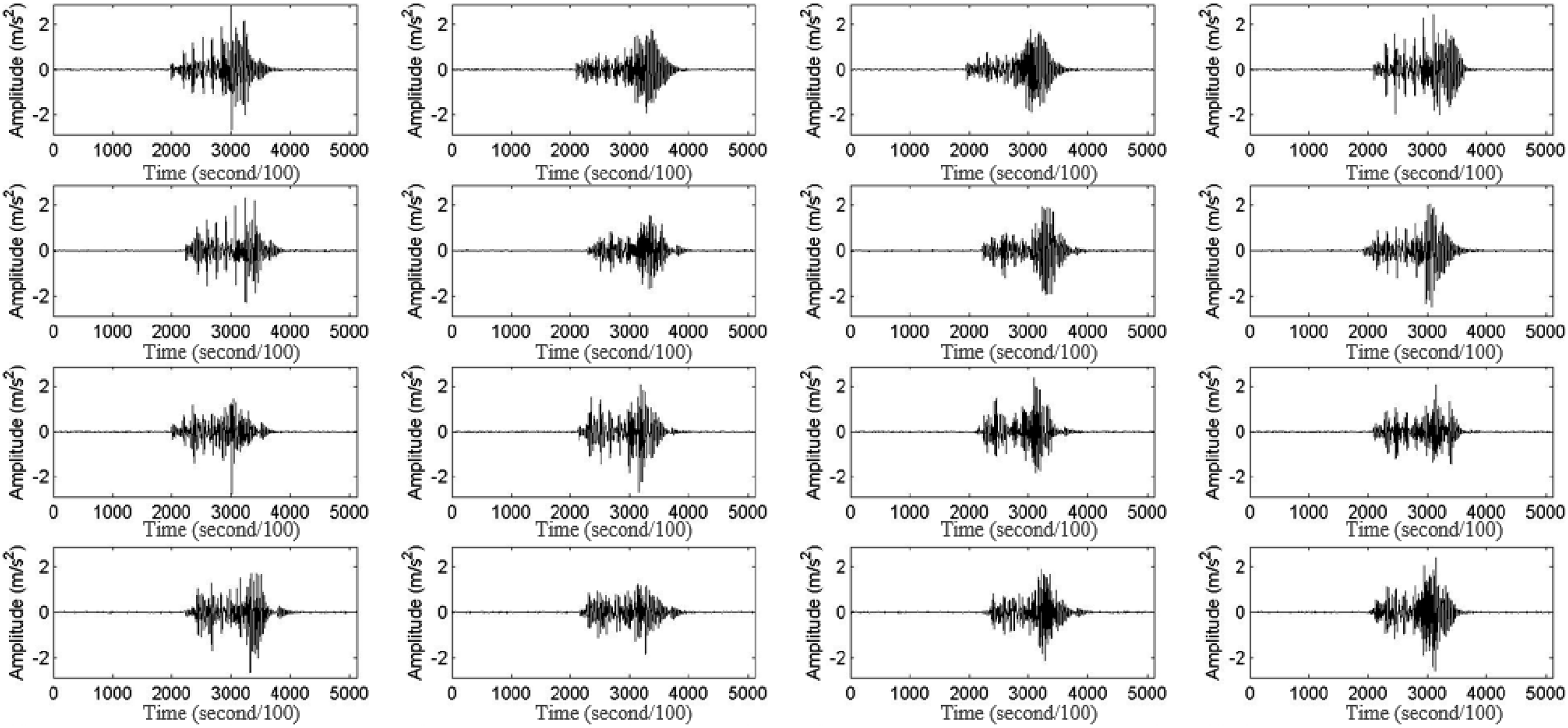

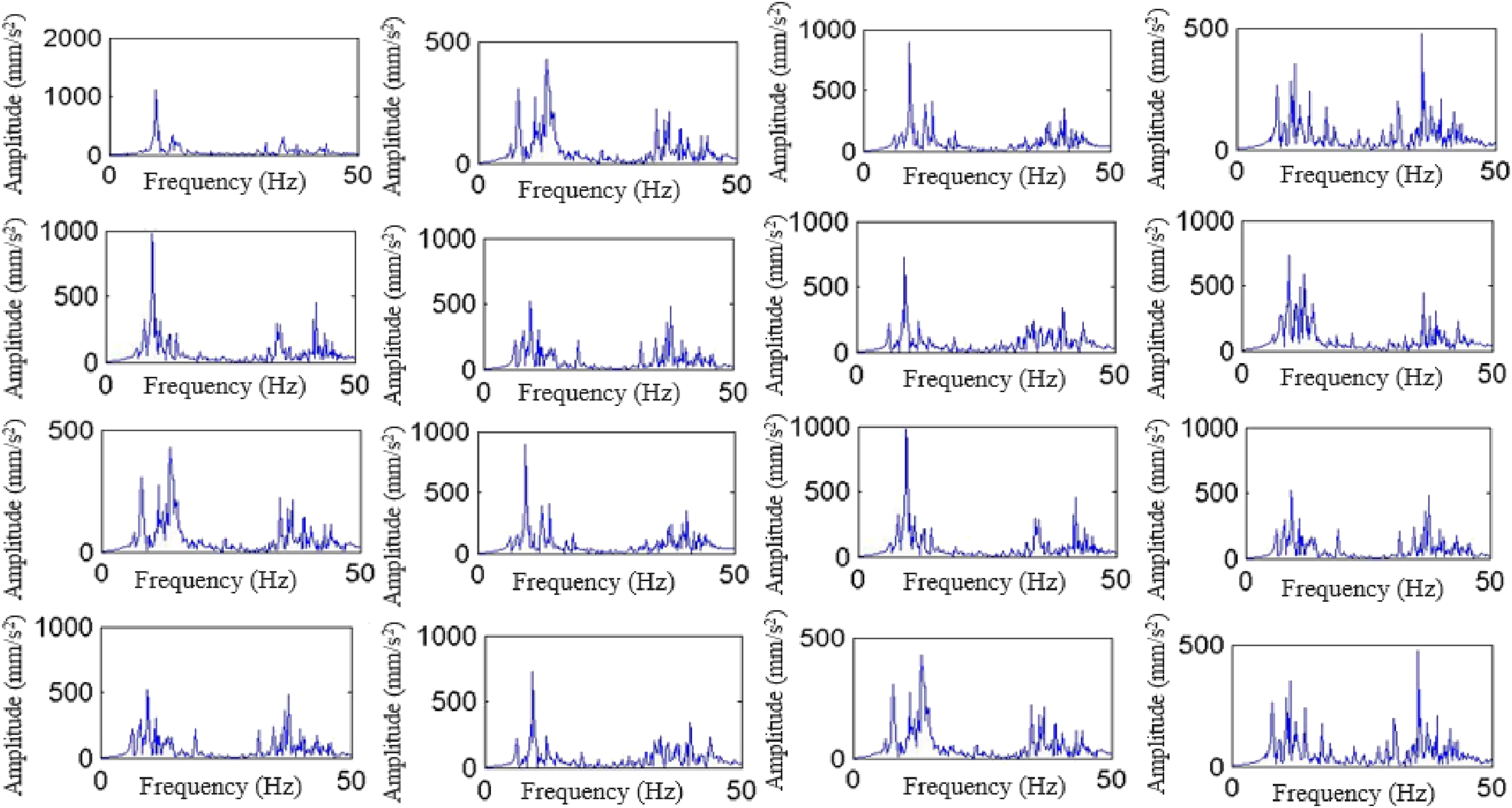
As analyzed in the theoretical section, assuming that the random load has a constant density function, the characteristics in the frequency domain will largely depend on the structural form function. The vibration acceleration signals obtained from the sensors at different positions are shown in Figure 17. The study cannot evaluate the differences through signals in the time domain because of the minimal changes in the original signal when the beam structure has defects. Furthermore, the characteristics of the original signal always depend on the load and the external conditions. Additionally, there are considerable noise and unwanted signals during the signal acquisition process. Therefore, the use of only the original signal characteristics during the beam vibration process cannot identify the appearance or growth of defects over time.

In contrast to the original signals obtained from the acceleration sensors, the vibration spectra of the signals obtained from Figure 16 are represented in Figure 17 through Fourier analysis. Observing the results as in Figure 17 shows the difference in the spectral shape in each boundary condition of the experimental beam structure. This difference reflects changes in the defect level, the velocity of movement and the movement of the load on the beam. To illustrate the differences in the spectral shape, two factors are considered: (1) the amplitude of the response frequency in the spectrum and (2) the value of that frequency. The difference in spectral amplitude between different measurement times is less considered in this study because it is a characteristic that depends on many influencing conditions and still contains noise during signal acquisition. Therefore, this study explores changes in spectral shape during changes in the external conditions on the structure. Depending on each state of the defect, this study proposes to evaluate changes in spectral shape as a feature of the process of assessing and monitoring structural degradation.

Changes in the area of the spectrum

Side defect of the beam

Defects in the structure are created by symmetric cuts 1.5 mm wide and 5 mm deep, with varying lengths of defect expansion. The test model is depicted in Figure 18, where the characteristic of this model is the active creation of defects on the beam side. This experimental method demonstrates the weakening of the beam structure models through the growth of defects in experimental cases along the width of the beam structure. This experimental model will be conducted in two cases: the first case with beams having the Ai defect arranged in the middle of the beam (with i being the level of growth of the defect in different experimental states) located between positions VT2 and VT3 as shown in Figure 19; and the second case with beams having two defects, in addition to the B_i defect similar to A_i located in the middle of VT1 and VT2, the second defect created is C_i placed between positions VT3 and VT4. The various defects in the beam structure in the study are shown in Table 4.

Figure 18.

Modeling a defect in a beam structure.

Figure 19.

Modeling two defects in a beam structure.

Table 4.

Level of side beam defects in Cases 1 and 2.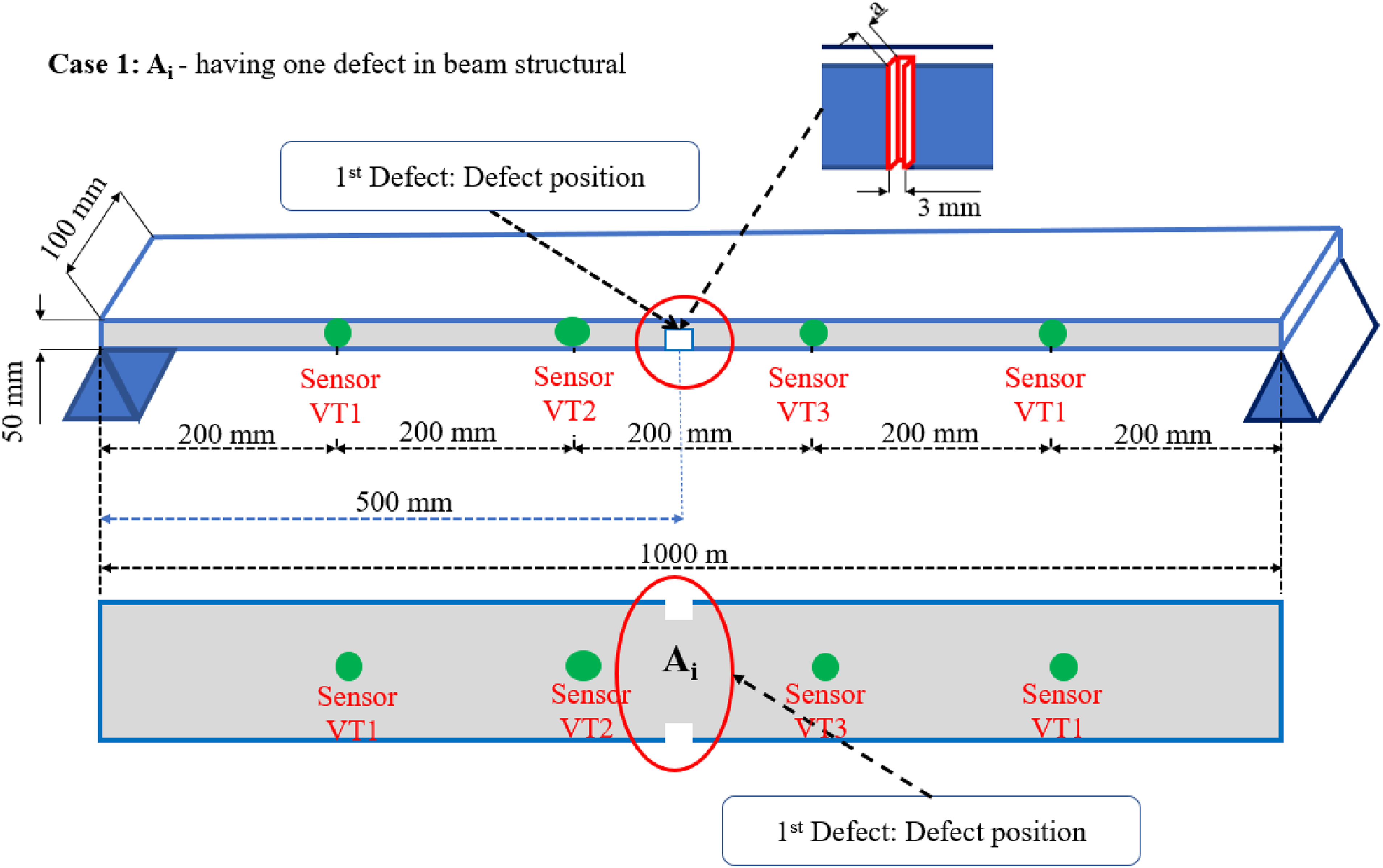

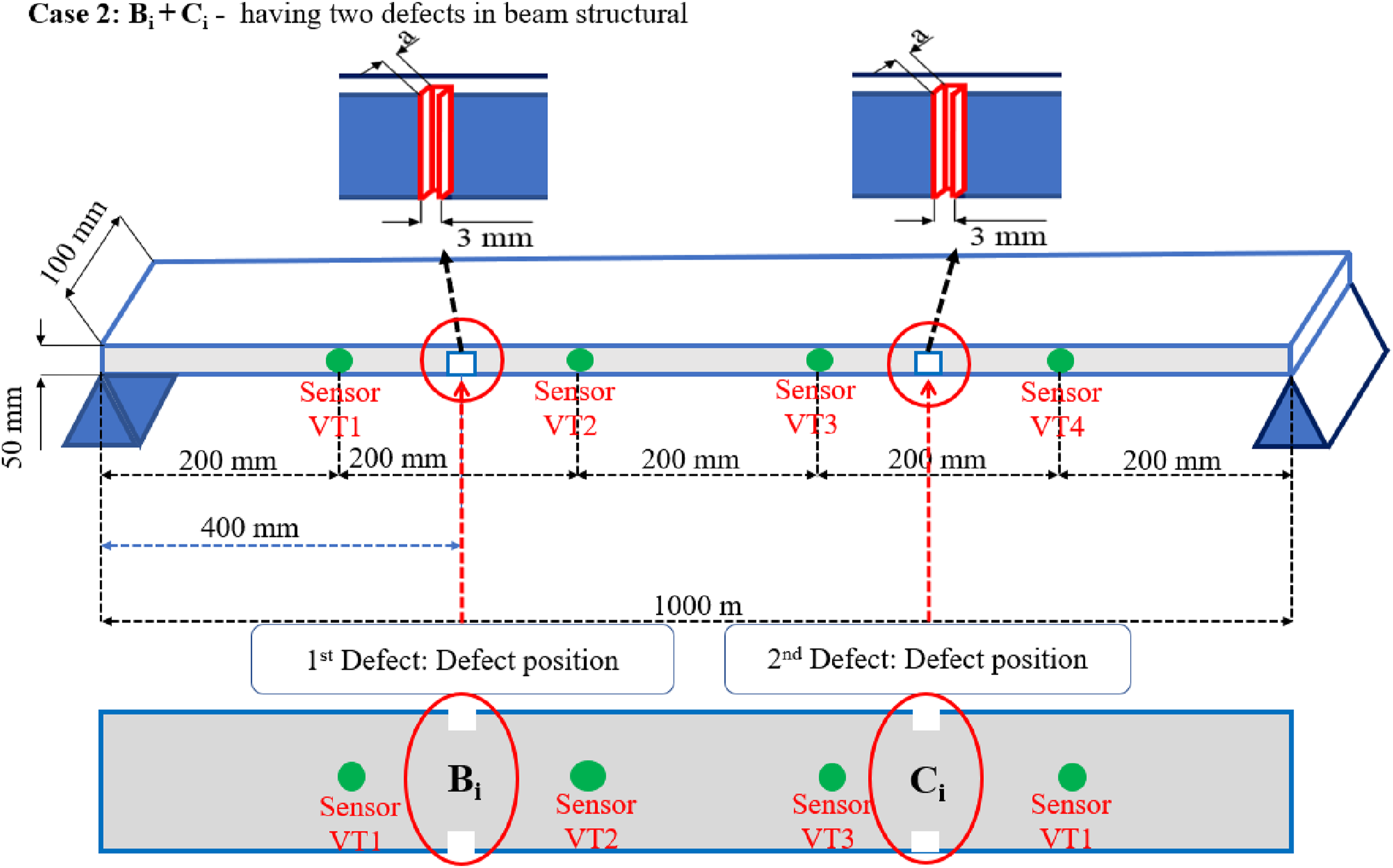
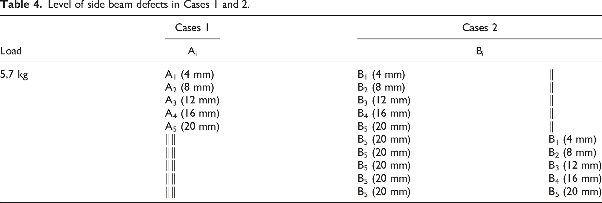
Load	Cases 1	Cases 2
	Ai	Bi
5,7 kg	A1 (4 mm)	B1 (4 mm)	‖‖
	A2 (8 mm)	B2 (8 mm)	‖‖
	A3 (12 mm)	B3 (12 mm)	‖‖
	A4 (16 mm)	B4 (16 mm)	‖‖
	A5 (20 mm)	B5 (20 mm)	‖‖
	‖‖	B5 (20 mm)	B1 (4 mm)
	‖‖	B5 (20 mm)	B2 (8 mm)
	‖‖	B5 (20 mm)	B3 (12 mm)
	‖‖	B5 (20 mm)	B4 (16 mm)
	‖‖	B5 (20 mm)	B5 (20 mm)

The minimum scale of damage that the proposed spectral moment analysis method can reliably detect was determined to be 4 mm in width and 5 mm in depth in beam structures, as demonstrated in the controlled laboratory experiments as shown in Table 4. This threshold reflects the smallest defect size that caused measurable changes in the M₀, indicating shifts in energy distribution across the frequency spectrum. However, for smaller defects, the method’s sensitivity is limited due to minimal energy redistribution and the influence of noise. Accurate detection at this scale is highly dependent on optimized sensor placement near damage-prone areas and maintaining a high signal-to-noise ratio (SNR). To enhance sensitivity to smaller-scale damage, future advancements could include the use of higher-order spectral moments, cumulative spectral moment models, and high-resolution sensors. These improvements would enable the method to detect even more subtle damage, extending its applicability to a broader range of structural health monitoring scenarios.

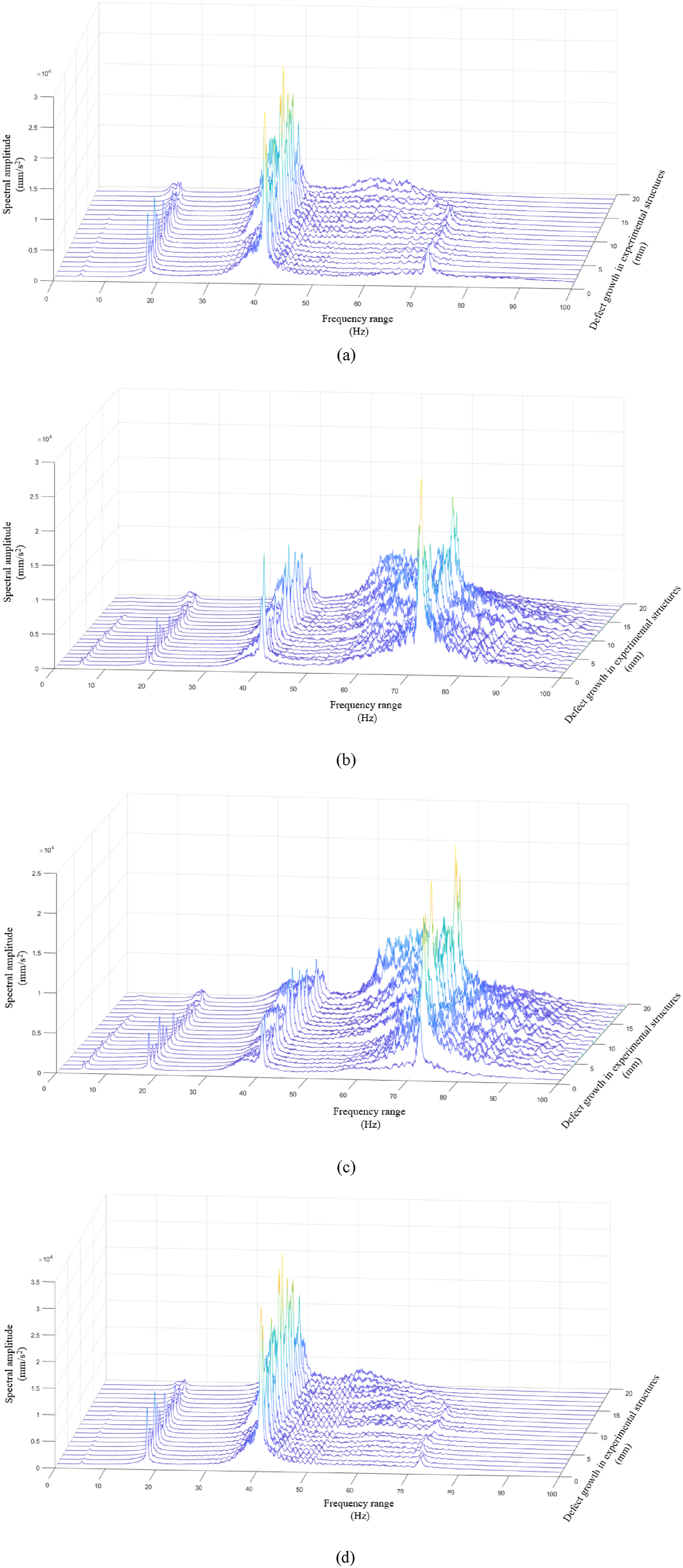
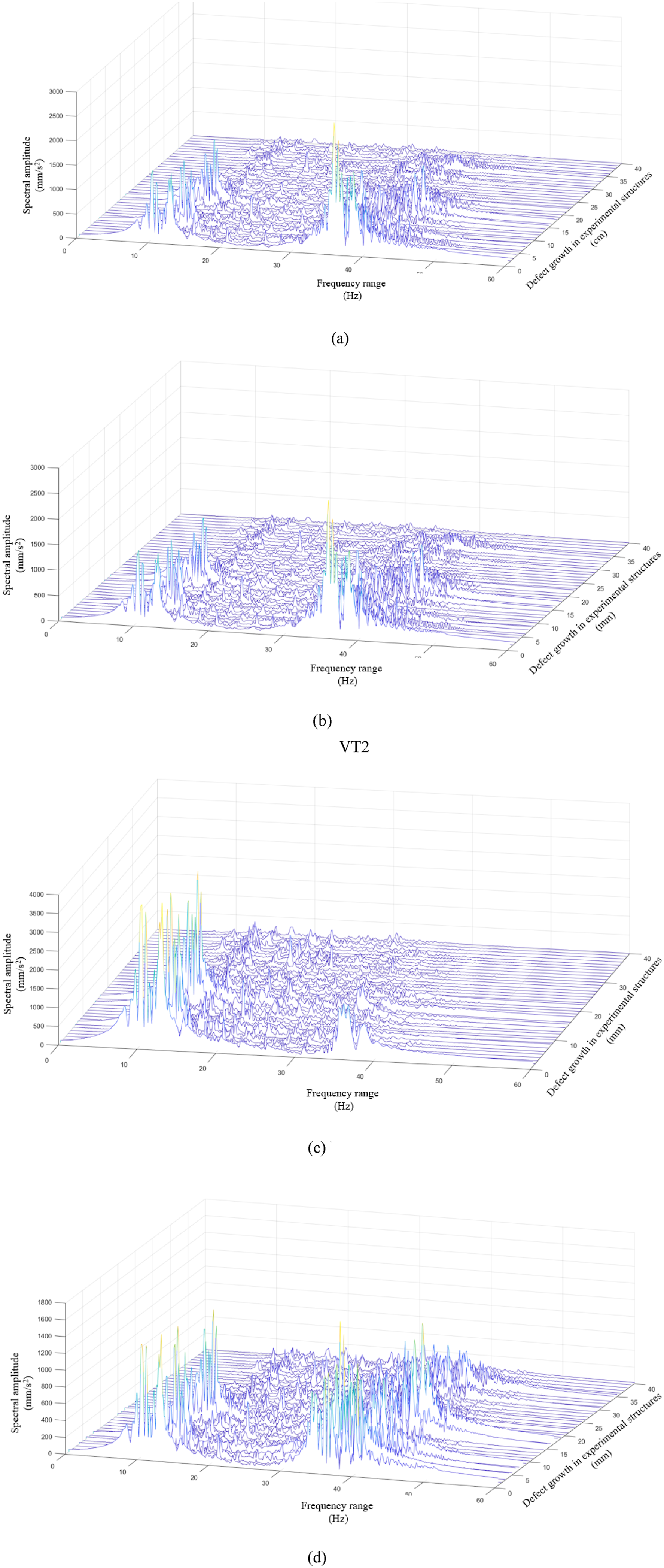
Similarly to Section 4.1, through the measurement of vibrations created by the moving load on the beam corresponding to different defective situations. The vibration spectra for each type of beam defect obtained are depicted in Figure 20 in Case 1 (a single beam defect) and Figure 21 in Case 2 (two beam defects). From Figures 20 and 21, it is observed that regardless of whether there are one or two defects, the vibration spectra always exhibit two dominant frequency regions, or so-called dominant frequency zones. The first frequency zone ranging from 7.5 to 15 Hz, with the highest spectral values typically concentrated around the range of 13 – 13.5 Hz. Similarly, the second frequency zone typically has a wider spectral spread ranging from 30 Hz to 48 Hz, with the highest frequency values usually concentrated around the range of 35-36 Hz. Besides these two dominant frequency zones, there also exists a region between these two frequency zones. To assess the presence of this region, this study posits it as the region containing noise or surplus energy values during the transition of defect states. Subsequent studies will dive into this third frequency zone. However, on the basis of the characteristics of these vibration spectra, the study draws the following evaluations.

- It is also observed that irrespective of the experimental case, the variation in the shape of the vibration spectrum always follows the rule that increasing the defect level progressively increases the spectral amplitude of the first vibration frequency zone. However, the frequency values of the experimental cases remain almost unchanged throughout the experiment. This implies that the spectral amplitude of the vibration is the primary factor reflecting the change in the shape of the spectrum under defect conditions and the development of defect levels. According to theoretical model analysis, this change in the shape of the spectrum represents the process of energy shifting from higher- to lower-frequency zones. Specifically, in this experiment, the study shows that the change in frequency amplitude shifts from higher- to lower-frequency zones.

- During the experiment, the shape of the vibration spectrum in Case 1 (with a defect located at VT2 and VT3) under the influence of defects created on the beam shows that all energy from the second frequency zone completely shifts to the first frequency zone, leading to a significant increase in the amplitude of the first frequency zone. Specifically, the vibration spectrum model at VT2 and VT3 with the second frequency zone has a much lower amplitude compared to the other two zones. This indicates that the influence of the defect only affects the positions around that defect without affecting the farther positions, specifically VT1 and VT4. Thus, the results of this study demonstrate that the change in spectrum image occurs only in the region where the defect exists and where the sensor is placed close to that defect. Furthermore, the strong energy shift from high- to low-frequency zones is a parameter capable of assessing the existence and development of defects in the structure.

- In contrast to Case 1, in Case 2, where defects are evenly distributed, the shape of the vibration spectrum does not change significantly, including the spectral values and amplitudes. The distribution of the vibration spectrum is symmetric on both sides. However, the results also show a strong shift of the high-frequency zone to the low-frequency zone, corresponding to the change in defects on the beam structure.

- From the above results, it is evident that the change in spectrum shape reflects the existence and growth of defects in different experimental states. This study also reveals the limitations of the spectrum identification model, that it can only detect major and non-cyclic defects and requires sensors to be placed close to the defects. In other cases, the study cannot detect the presence of defects.

Figure 20.

Relationship between vibration spectrum and defect growth in beam structures in Case 1. (a) Visual change of the vibration spectrum with the growth of a defect in the beam at position VT1. (b) Visual change of the vibration spectrum with the growth of a defect in the beam at position VT2. (c) Visual change of the vibration spectrum with the growth of a defect in the beam at position VT3. (d) Visual change of the vibration spectrum with the growth of a defect in the beam at position VT4.

Figure 21.

Relationship between vibration spectrum and defect growth in beam structures in Case 2. (a) Visual change of the vibration spectrum with the growth of two defects in the beam at position VT1. (b) The visual change of the vibration spectrum with the growth of two defects in the beam at position VT2. (c) Visual change of the vibration spectrum with the growth of two defects in the beam at position VT3. (d) Visual change of the vibration spectrum with the growth of two defects in the beam at position VT4.

Investigation of the zero-order spectral moment (M₀)

As analyzed above, it is clear that the variation of the spectrum shape can represent the ability to assess the presence of defects in the beam structures and the growth of those defects in each experimental case. To investigate changes in the vibration spectrum between defect levels, the study divided the frequency domain into regions corresponding to the first observable frequency region on the frequency spectrum. The results from Figure 22 show that the width of the spectrum in Case 1 ranges from 7.5 to 15 Hz, with the maximum spectral value typically concentrated around the range of 13 to 13.5 Hz. Similarly, in the second frequency region, the spectrum width typically extends from 30 to 48 Hz, with the maximum frequency value typically concentrated around the range of 35-36 Hz, as depicted in Figure 22 for the cases of single defect beam, and Figure 23 shows the results of a beam with two defects.

Figure 22.

Relationship between vibration spectrum and defect growth in beam structures in Case 1. (a) The area of the vibration spectrum changes with the growth of a defect in the beam at location VT1. (b) The area of the vibration spectrum changes with the growth of a defect in the beam at location VT2. (c) The area of the vibration spectrum changes with the growth of a defect in the beam at the location VT3. (d) The area of the vibration spectrum changes with the growth of a defect in the beam at the location VT4.

Figure 23.

Relationship between vibration spectrum and defect growth in beam structures in Case 2. (a) The area of the vibration spectrum changes with the growth of two defects in the beam at location VT1. (b) The area of the vibration spectrum changes with the growth of two defects in the beam at location VT2. (c) The area of the vibration spectrum changes with the growth of two defects in the beam at location VT3. (d) The area of the vibration spectrum changes with the growth of two defects in the beam at location VT4.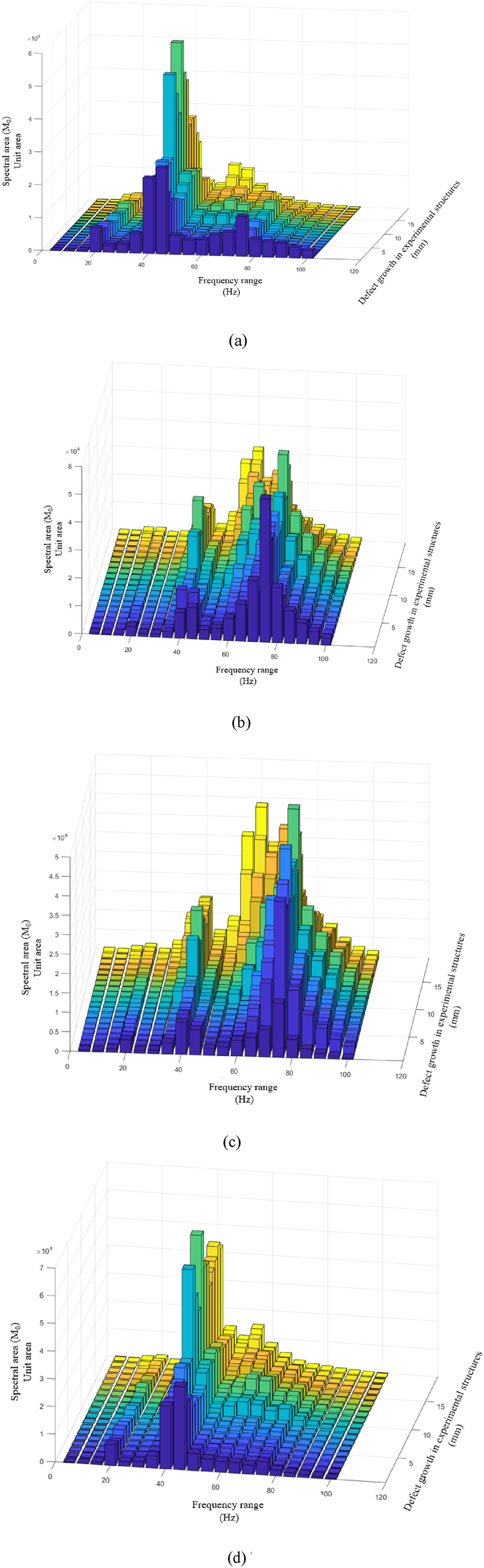

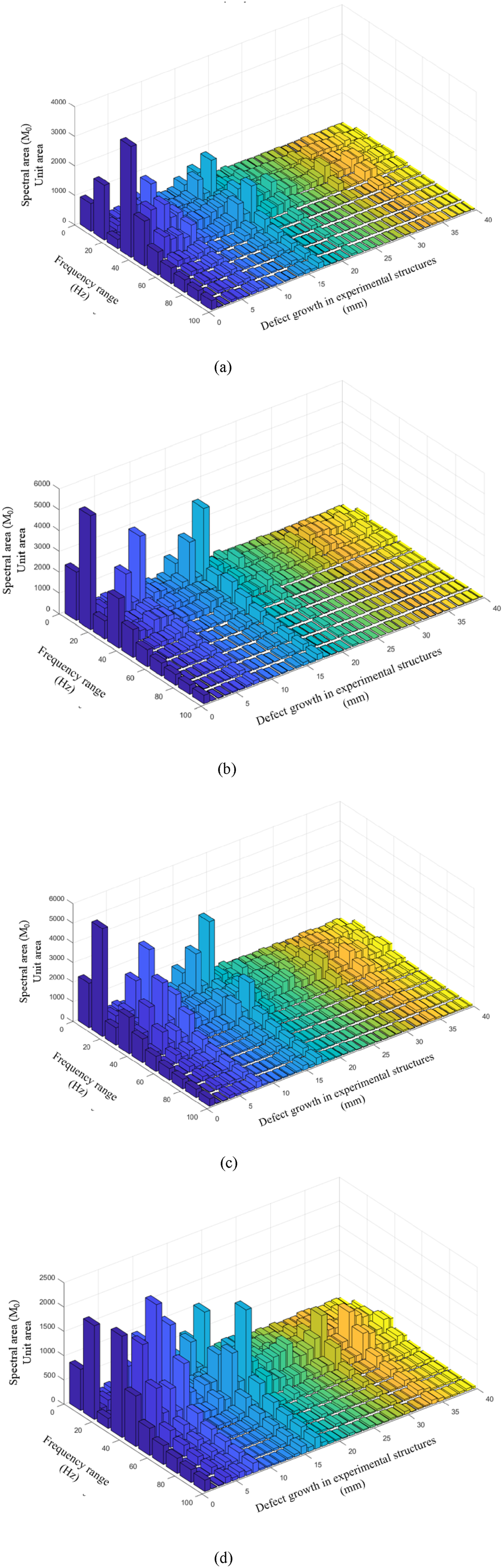
The results in Figure 22 show that the M₀ value extracted from the vibration spectrum of the model through experiments as shown in Figures 18 and 19, indicates the length of the frequency ranges in the first region ranging from 7.5 to 15 Hz and the frequency range in the second resonance region ranging from 30 to 48 Hz, at all sensor positions Vti and there is a decreasing trend in amplitude with the growth of the defect. The M₀ value reflects the variation in the area of the vibration spectrum that corresponds to different defect states in both models:

- The M₀ value whether there is only one defect or multiple defects on the beam, at all VTi positions, showing that its amplitude decreases with increasing experimental defect levels. Specifically, when the defect level reaches 15 mm, it enters the stage of decreasing area in the frequency ranges. Figure 22(a)-(d) show that at four different VTs, in the initial stage (when the beam defect is small), the change in the spectrum area is insignificant. However, when the defect influence level is high, meaning that the defect extends in the beam, the spectrum area decreases and completely disappears for 20 mm in Case 1 and 40 mm in Case 2 (the sum of two damages). Also, for the case of two defects in the beam, the M₀ value decreases much faster than in the model with one defect.

- The difference in Case 1 is that VT1 and VT4 have only one area, while VT2 and VT3 always have two areas at the frequency region values of 40 Hz and 70 Hz, respectively. This shows that the position of the defect will greatly affect the change in the shape of the vibration spectrum of the structure through the M₀ spectral moment model. Meanwhile, in Case 2 with two beam defects, the change in the M₀ value also occurs similarly at the four different positions. This indicates that the M₀ model can be very sensitive to the presence of defects in the beam, as well as to evaluate the growth of those defects over time or in terms of defect expansion.

- The primary differences between Figures 20–23 lie in the representation of the structural response at varying levels of damage and within different frequency ranges. Figures 20 and 21 depict the overall frequency spectra for different damage conditions, showing how the spectral shape evolves as the damage level increases. In contrast, Figures 22 and 23 focus on specific frequency bands that highlight significant shifts in the vibration spectra, which are crucial for identifying the progression and extent of damage. The frequency bands in Figures 22 and 23 differ because they represent different stages of damage progression. As the damage intensifies, energy shifts from one frequency band to another, which is reflected in the changes to the width and location of the frequency bands between these figures. The process of identifying the width of these frequency bands was based on the analysis of the cumulative spectral moment values. We determined the bands by observing where the most significant energy shifts occurred as damage levels increased. The width of each band correlates with the frequency zones where the amplitude variations were most pronounced, providing key insights into the structural health and damage progression at each stage.

The drawback of this M₀ model is that it cannot detect the presence of defects when the defect value is still low, meaning that, although it can serve as an indicator of the presence of the defect, the defect level must be large enough for the M₀ model to clearly detect its presence. Because in the range of small defect values, the variation of the M₀ value is not clear and the change in value is insignificant compared to expectations. Therefore, new methods must be proposed to be able to identify the presence of defects in the early stages.

For a continuous system, the power spectrum at each defect position also depends on the shape of each vibration mode at that position, as theoretically analyzed in Section 2.4.2. To assess the relationship between the change in the value of the spectral moment at different positions corresponding to the growth level of the defect, if the study only considers the relative value of the spectral moment with the growth of the defect, it can be expressed as follows equation (38):

$\mathrm{\Delta }{M}_{i\left(n\right)}=\frac{{M_i}_{\left(n\right)}-{M_1}_{\left(n\right)}}{M_{1\left(n\right)}}$

(38)

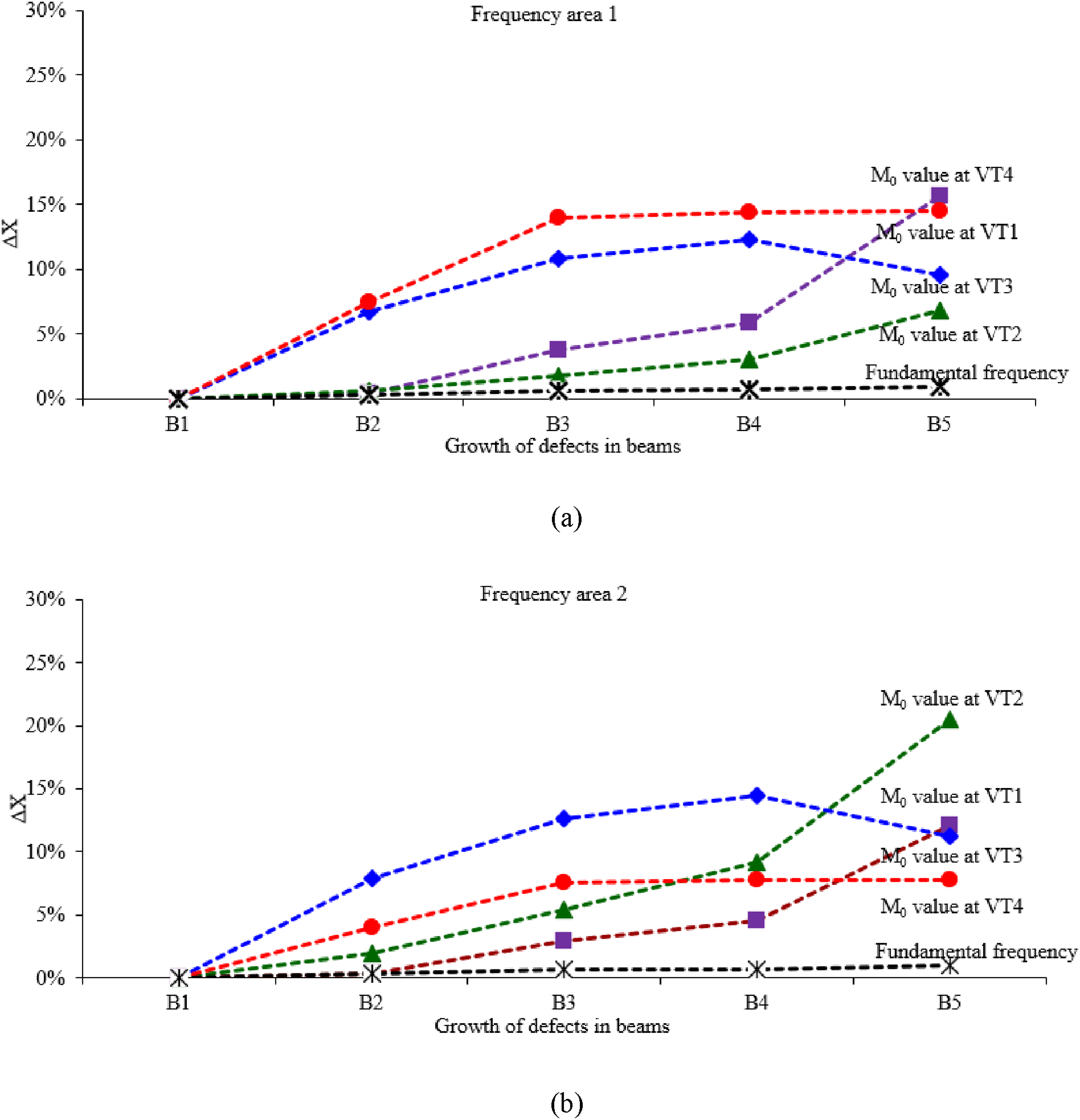
The results of Figures 24 and 25 of the study indicate that at all four positions, the value of ΔM₀ for region one will increase proportionally with the degree of growth of the defect. Similarly, ΔM₀ for region two will decrease with the degree of growth of the defect. This means that when the structure contains multiple defects or the defects are sufficiently large, almost all of the energy of the vibration spectrum from this region will shift to the first frequency region and disappear completely when the defect level becomes large enough. From an overall perspective, as the defect grows, the relative values of the M₀ spectral moment for both regions (the difference values between two states) increase at all four positions. When the defect grows to states A3 and B5, the ΔM₀ values at all positions change by more than 5%, while the natural frequency changes only by 1%. This shows that the ΔM₀ index increases much more than the change in natural frequency, as clearly shown in Figures 24 and 25. This indicates that the ΔM₀ spectral moment index is much more sensitive than the natural frequency in the identification of defects, according to the theory of spectral moments of continuous systems. Furthermore, the study also clarifies how the use of the spectral moment value helps investigate characteristics for an effective and rational assessment of damage.

Figure 24.

Changes in ΔM ₀ for frequency region one and frequency region 2 with the degree of growth of the defect in Case 1. (a) Relationship between area change and defect growth in frequency area 1 in case 1. (b) Relationship between the change in area and the growth of the defect in frequency area 2 in case 1.

Figure 25.

Changes in ΔM ₀ for frequency region one and frequency region 2 with the degree of growth of the defect in Case 2. (a) Relationship between area change and defect growth in frequency area 1 in case 2. (b) Relationship between area change and defect growth in frequency area 2 in case 2.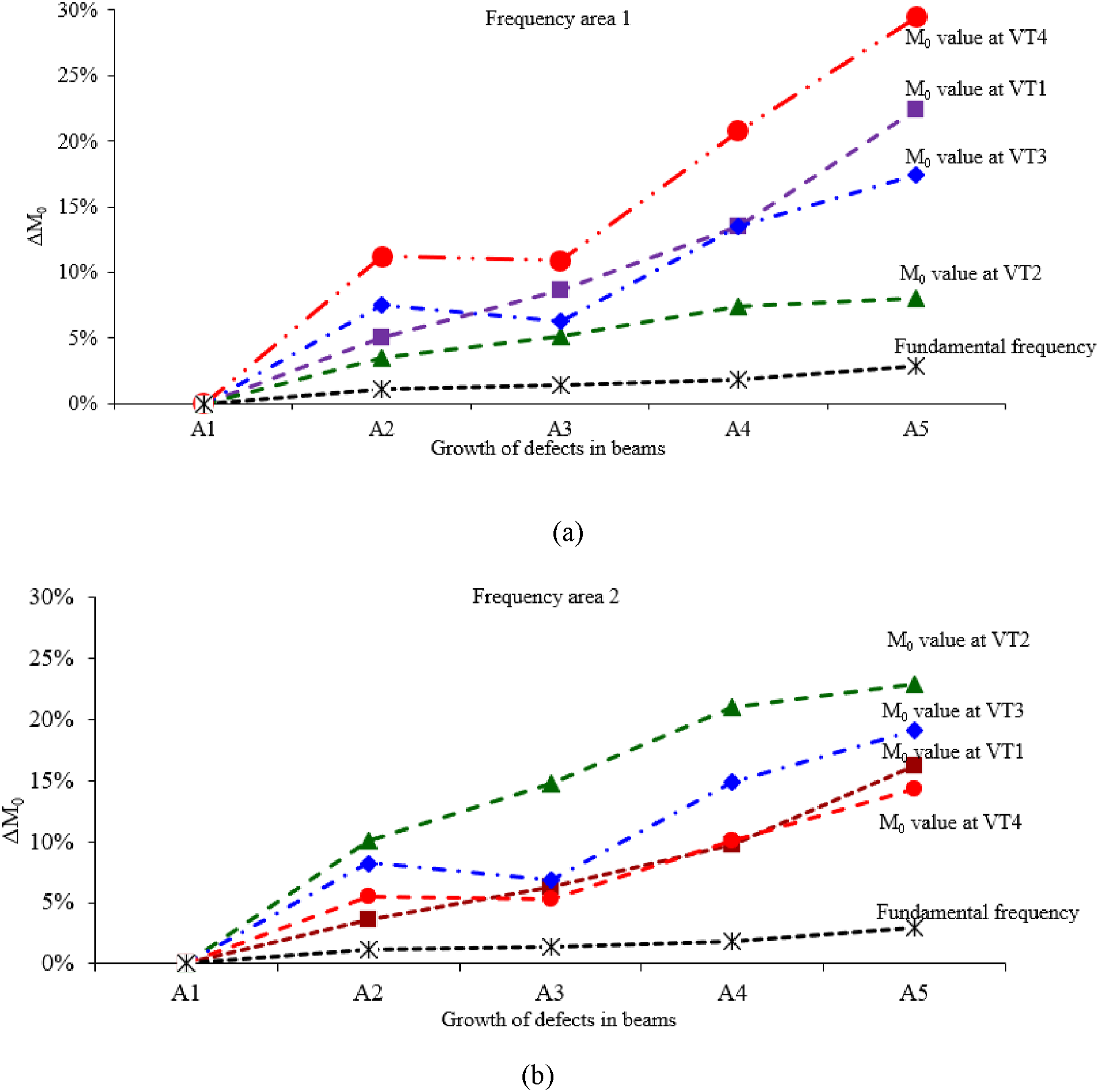

The spectral moment analysis approach offers the potential to estimate the remaining service life of a structure by tracking damage progression and quantifying structural degradation. The zeroth-order spectral moment (M₀) is highly sensitive to changes in energy distribution caused by structural damage, such as reductions in stiffness or increases in damping. By monitoring trends in M₀ values over time, this method provides critical insights into the progression of cracks, corrosion, or fatigue. Additionally, integrating spectral moment analysis with predictive models—such as machine learning or finite element simulations—can enhance its capability to forecast structural performance and estimate failure thresholds. While this study primarily focuses on detecting and localizing damage, future work could establish direct correlations between spectral moment trends and service life, enabling a comprehensive framework for lifecycle prediction and maintenance planning.

Cumulative model of spectral moment values

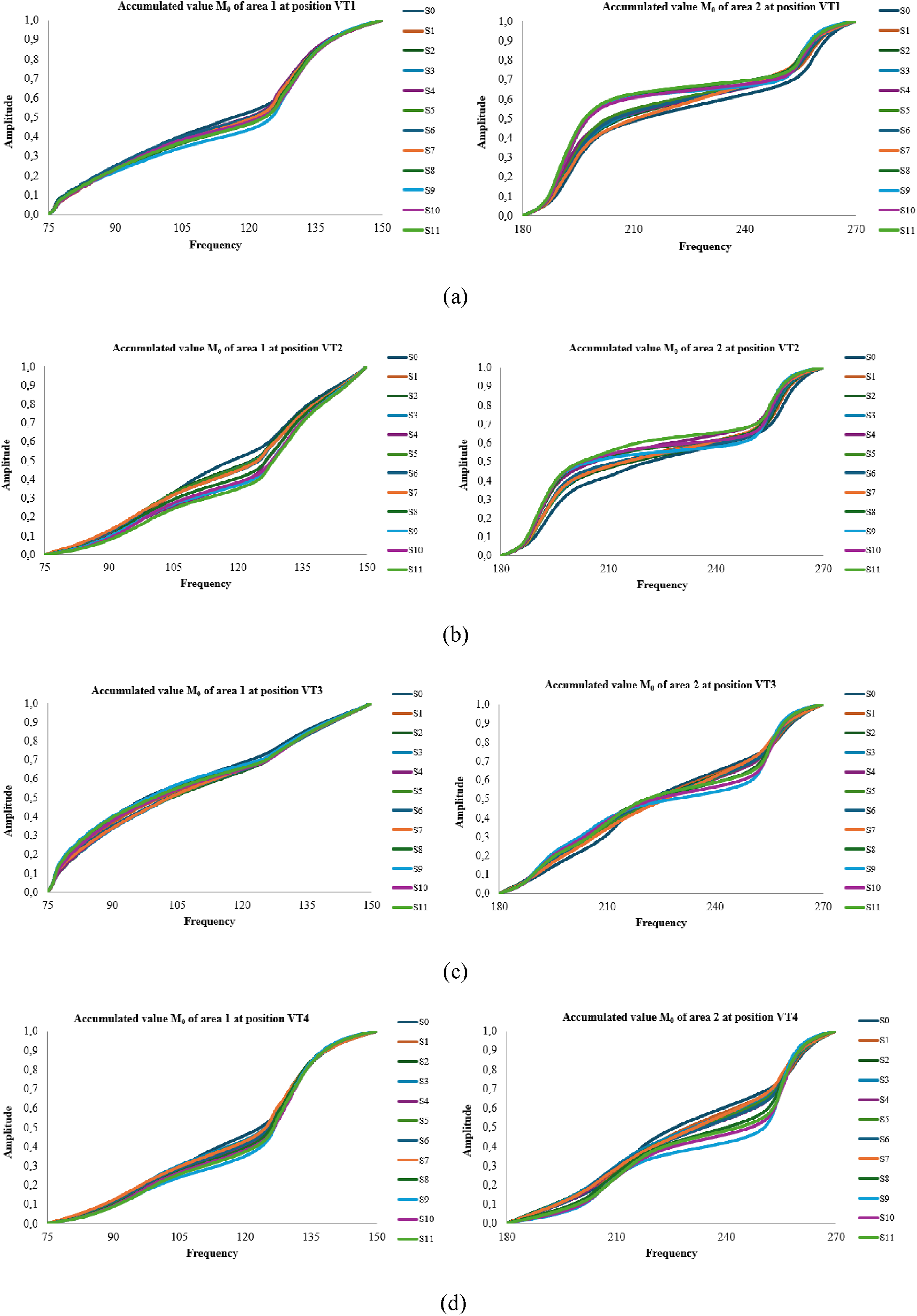
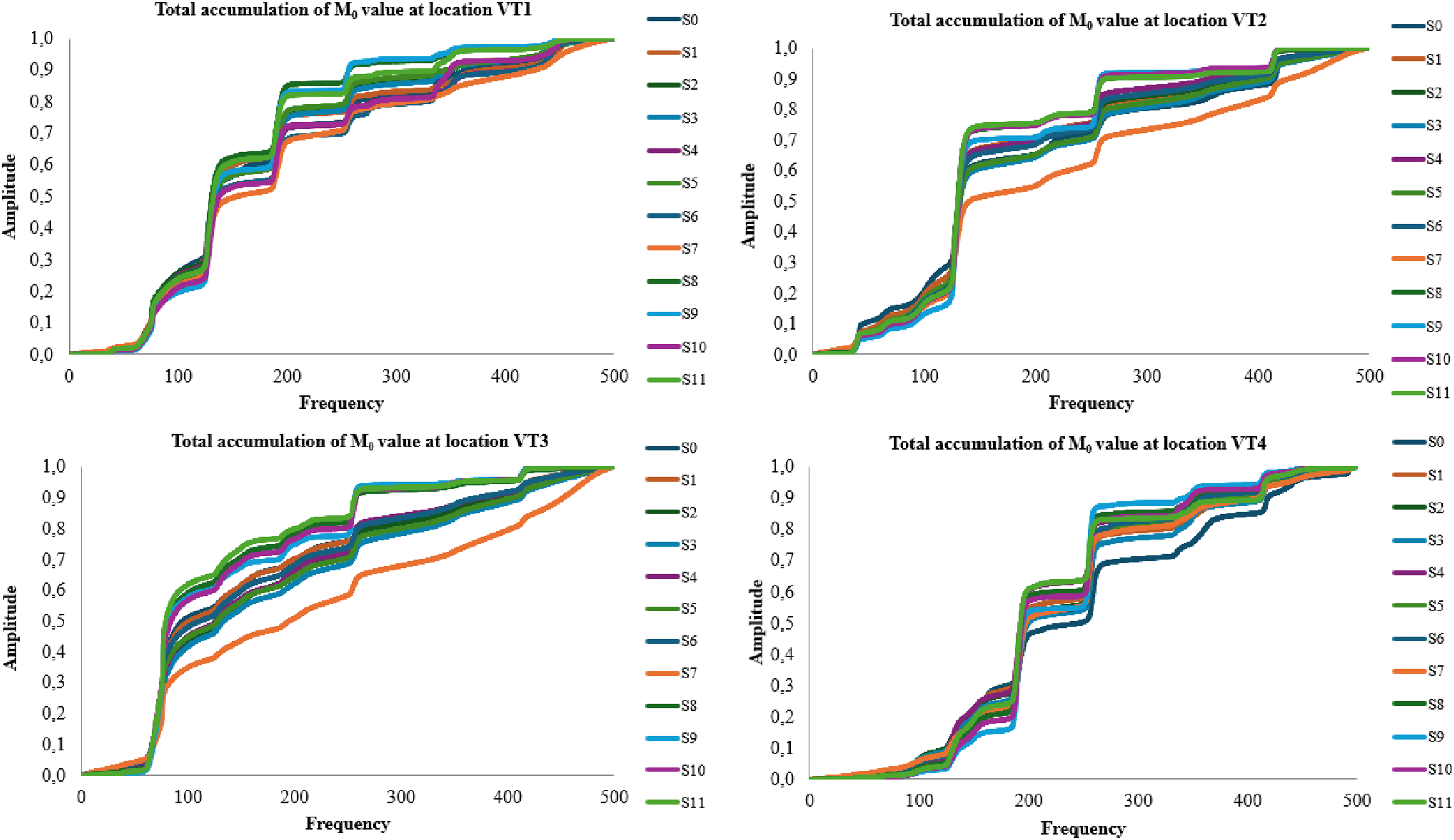
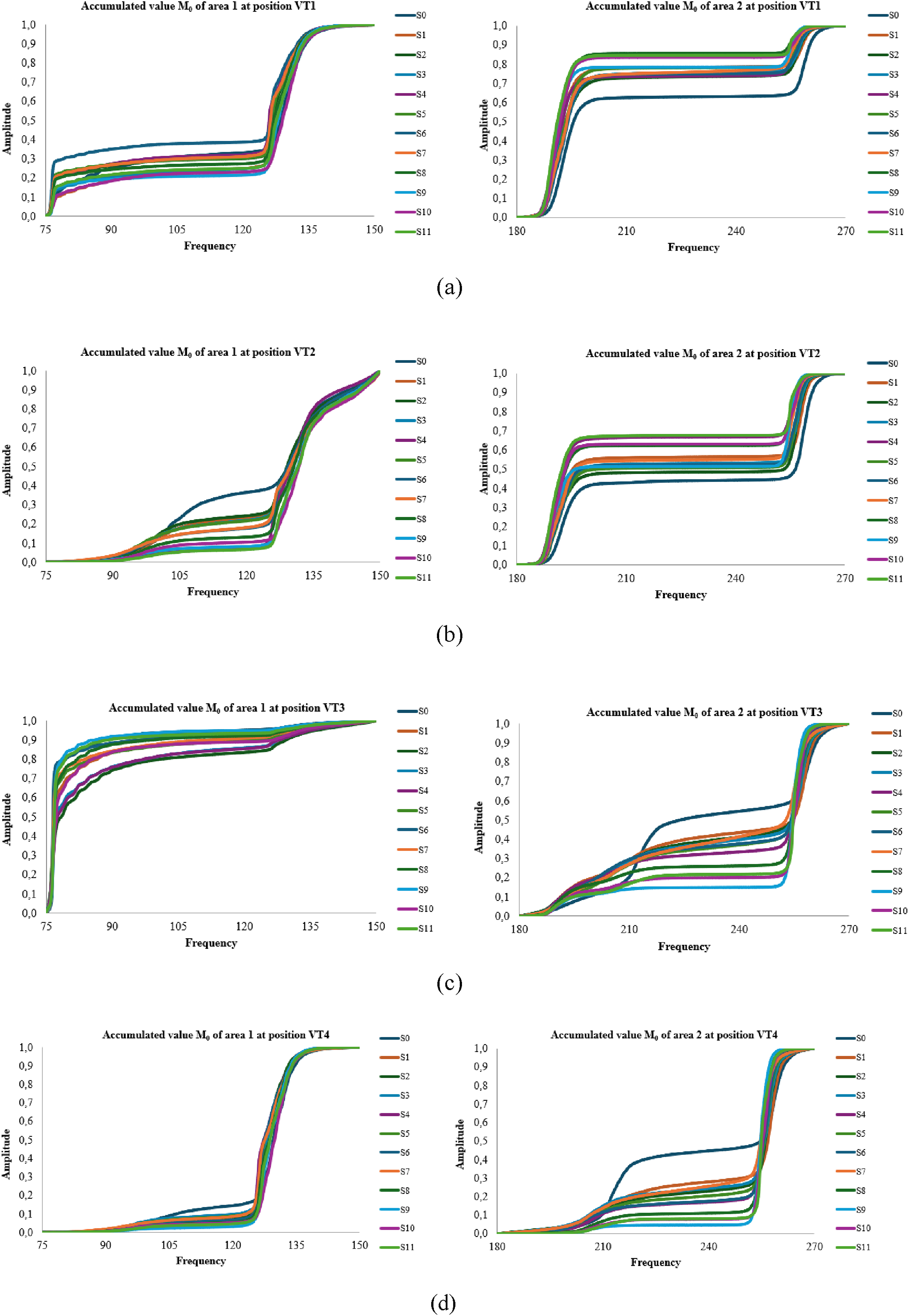
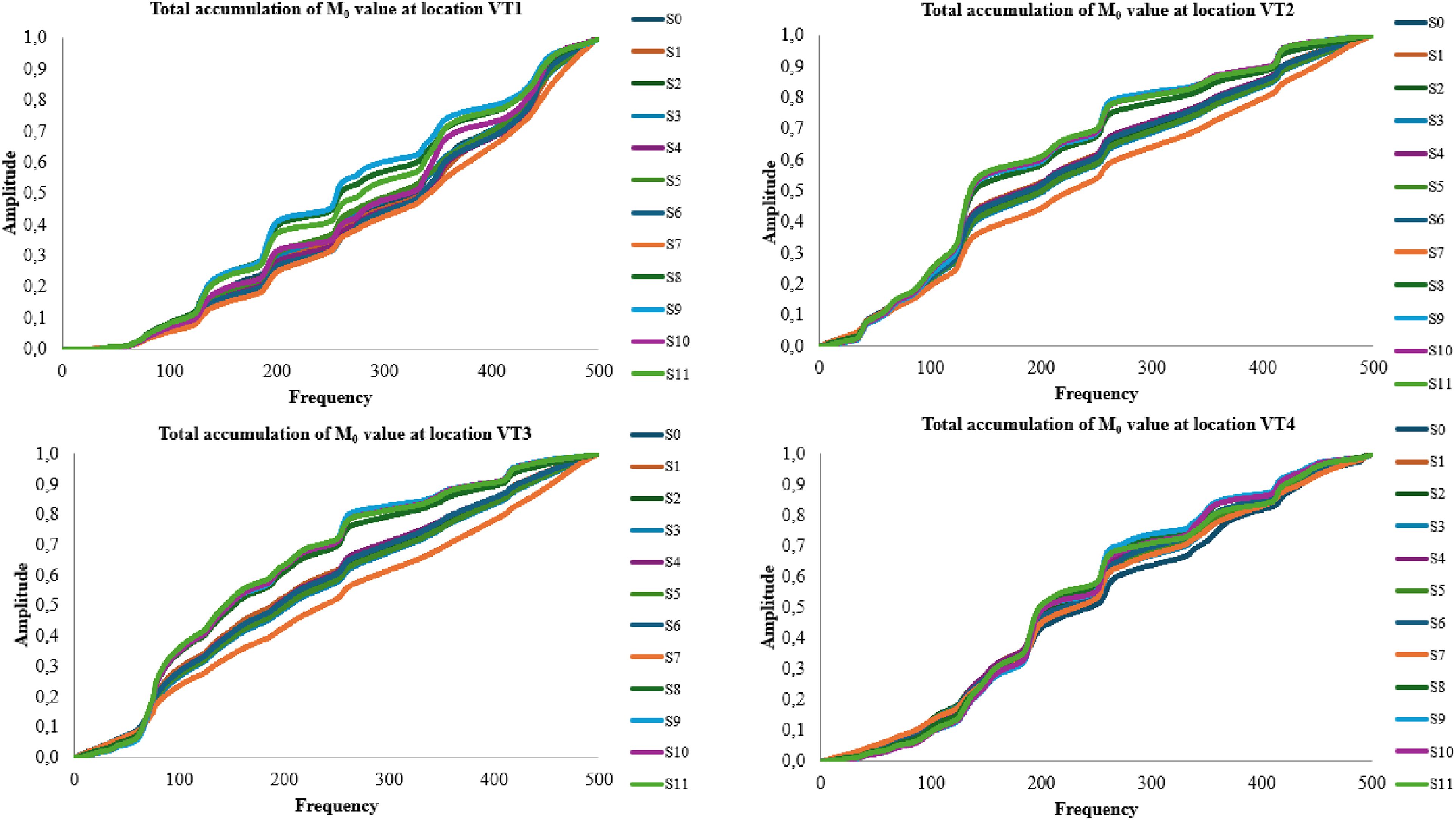
As discussed above, the advantage of the M₀ spectral moment model is its sensitivity to the presence and development of defects within the structure. However, it cannot be denied that the M₀ model can only accurately and sensitively detect defects when the defect level is sufficiently high to affect the shape of the vibration spectrum, thus altering the M₀ spectral moment values. This study proposes an additional model that calculates the cumulative values of M₀ moments to demonstrate and identify structural damage early on.

- Figures 26–29 illustrate the cumulative spectral moment values (M₀) at various stages of damage progression along the beam. These figures allow the identification of specific defect locations by tracking changes in the spectral moment values corresponding to different levels of damage. As the damage level increases from S1 to S11, significant shifts in the cumulative M0 values are observed. These changes help pinpoint the areas of the beam where damage has occurred, as spectral moment values are sensitive to variations in the structural response. Localized shifts in the cumulative M₀ values reflect areas with defects, enabling the detection of both the location and severity of the damage. Therefore, by analyzing the cumulative spectral moment values at each damage stage (S1–S11), we can identify how the damage progresses and where it is concentrated.

- The terms S1–S11 in the figure legend represent the increasing levels of damage applied to the beam during the experiment. S1 corresponds to the lowest level of damage, while S11 represents the highest level of damage that could be introduced in this experiment. These stages describe a gradual progression of defects, allowing us to examine how the structural response changes as the damage becomes more severe. The cumulative M0 values at each stage reflect the extent of damage, with more pronounced changes at higher levels of damage (e.g., S11), indicating significant structural deterioration

- Using the cumulative model of the spectral moment values (M₀), it can be demonstrated that structural weakening mainly depends on its overall stiffness from Figures 25 and 27, the differences between the single-defect model (Model 1) and the dual-defect model (Model 2) are clearly evident. For the single defect case, VT1 and VT4 are hardly affected by defects during operation due to similar and slow accumulation processes at these positions. On the contrary, for VT2 and VT3, changes in the accumulation process of M₀ spectral moment values occur abruptly and rapidly, especially in the second resonant region within the frequency range. In the case of the dual defect beam model, changes in the accumulation process can easily identify the presence and growth of defects in the structure, since accumulation occurs rapidly and intensively when the structure has multiple defects as Figures 26 and 28. This demonstrates that this model is suitable for theoretical analysis, since the spectral moment values directly depend on the overall stiffness through the vibration spectrum.

- This cumulative spectral moment value model demonstrates its importance as an important analytical tool in the field of structural engineering, especially in research on the impact of defects on beams. By using this model, researchers can fully understand and describe how defects affect the structure over time because the cumulative spectral moment value model enables the identification of specific defect locations on the beam. This is crucial, as the location of the defect can influence the response of the beam under load, thus affecting structural integrity.

Figure 26.

The model accumulates the spectral moment of four VT in Case 1. (a) The model accumulates the spectral moment value M₀ at VT1 in case 1. (b) The model accumulates the spectral moment value M₀ at VT2 in case 1. (c) The model accumulates the spectral moment value M₀ at VT3 in case 1. (d) The model accumulates the spectral moment value M₀ at VT4 in case 1.

Figure 27.

Relationship between the total spectral moment accumulation model and defect growth at the 4 VT locations in Case 1. (a) The model accumulates the spectral moment value M₀ at VT1 in case 2. (b) The model accumulates the spectral moment value M₀ at VT2 in case 2. (c) The model accumulates the spectral moment value M₀ at VT3 in case 2. (d) The model accumulates the spectral moment value M₀ at VT4 in case 2.

Figure 28.

The model accumulates the spectral moment of four VT in Case 2.

Figure 29.

Relationship between the total spectral moment accumulation model and defect growth at the four VT locations in Case 2.

Conclusions, limitations and future research directions

Conclusions

This study presents a comprehensive approach using spectral moment analysis and cumulative spectral moment models to enhance the detection and evaluation of structural damage in beam structures. The primary objective was to develop an effective, cost-efficient method to identify the location, type, and extent of damage, particularly in early stages where traditional methods may fall short. The experimental results achieved this objective by demonstrating that spectral moment values, specifically the zeroth-order moment (M₀), are highly sensitive indicators of damage. These values accurately reflect shifts in energy distribution from higher to lower frequency zones, highlighting the presence and progression of structural issues.

The cumulative spectral moment model further strengthens this analysis by enabling detailed tracking of how damage evolves over time and pinpointing affected areas. The findings underscore that this approach can detect damage with precision and offer timely insights that facilitate prompt repair or maintenance. This reinforces the model’s potential as a practical tool for structural health monitoring, capable of improving safety, minimizing risk, and extending the lifespan of engineering structures.

Moreover, conducting the research in a controlled laboratory setting proved the model’s practicality by reducing costs and analysis time compared to prior studies. However, the study also notes limitations in detecting minor or non-repetitive defects when sensors are positioned far from the damage site, suggesting future research should explore enhanced sensor placement strategies.

In conclusion, the alignment of this method with the manuscript’s objectives is clear: it provides an innovative, scalable solution for real-time structural damage assessment. The results offer a foundation for future applications and adaptations in various engineering contexts, supporting more reliable decision-making regarding repair, reinforcement, or replacement of damaged components. This research solidifies the spectral moment analysis as a significant contribution to advancing structural health monitoring methodologies.

Limitations

This study primarily focuses on using spectral moment analysis for detecting and localizing structural damage, without directly addressing the estimation of remaining service life. A key limitation is the lack of established correlations between spectral moment trends and structural failure criteria, which are essential for predicting service life. Additionally, the study does not account for environmental and operational variability, such as temperature fluctuations or dynamic loading conditions, which can significantly influence the progression of structural damage.

Future research directions

Future research will focus on extending the spectral moment analysis framework to estimate the remaining service life of structures. This includes developing robust correlations between spectral moment trends (e.g., zeroth-order spectral moment M0) and structural failure thresholds. Integration with predictive models, such as machine learning algorithms and finite element simulations, will enable more accurate lifecycle predictions. Moreover, incorporating the effects of environmental and operational factors into the analysis will enhance the method’s applicability in real-world scenarios, making it a comprehensive tool for structural health monitoring and maintenance planning.