Sage Journals: Discover world-class research

Abstract

This article presents a hybrid control method for an automotive suspension system to improve smoothness and comfort and eliminate the influence of sensor noise. The proposed algorithm is formed by combining an active disturbance rejection control technique and a dynamic fuzzy technique based on an extended state observer. The article’s novel contribution is to propose a solution for determining a reference signal and adjusting control parameters using soft computing techniques. Simulations are performed in three cases (corresponding to three types of road excitation signals) to validate the performance of the proposed algorithm. According to the calculation results, the displacement and acceleration of the vehicle body are significantly reduced when the proposed technique is applied to control the active suspension system. The error of the road disturbance observed by the extended state observer does not exceed 0.5 mm, while the error of the vehicle body displacement is less than 0.001 mm. In addition, the chattering phenomenon caused by sensor noise is completely eliminated once the proposed algorithm controls the active suspension system. In conclusion, the algorithm introduced in this work provides superior performance over traditional control methods, which is validated by simulation results.

Keywords

Active suspension system active disturbance rejection control dynamic fuzzy sensor noise

Introduction

Road roughness is one of the many sources of vehicle vibrations, directly affecting ride comfort. A traditional passive suspension system cannot provide sufficient performance in controlling vehicle vibrations. As a result, ride comfort and handling stability are severely degraded under severe driving conditions. Nowadays, conventional passive suspension systems are gradually being replaced by controllable suspension systems to improve ride comfort and road holding. According to Nguyen and Nguyen, controllable suspension systems are classified into active suspensions with hydraulic actuators or linear motors, semi-active suspensions with magnetorheological dampers, and pneumatic suspensions.¹ Active suspension systems provide superior performance in controlling vehicle vibrations compared to the other two systems. The hydraulic actuator of the active suspension system operates based on the displacement of hydraulic servo valves, which are controlled by a predefined controller.²

Literature review

Active suspension systems are controlled by various methods. Each control method depends on the type of system, the control object, and the control target. The proportional integral derivative (PID) algorithm is suitable for linear single input and single output (SISO) systems. In Ref. 3, Haemers et al. designed a PID controller to control a full suspension model. The system parameters were optimized by a genetic algorithm (GA). However, the sprung mass acceleration was massive, exceeding 15 m/s². Another optimization method called ant colony optimization (ACO) was applied to find PID gains for the suspension system, which was introduced by Gad et al.⁴ This algorithm was inspired by a biology mechanism based on identifying the movement of ants across nodes. The simulation showed that the sprung mass acceleration was reduced, but the signal was delayed in phase. Another method used to tune the optimal parameters for PID control was proposed in Ref. 5, known as the advanced firefly algorithm (AFA). Talib et al. concluded in Ref. 5 that vehicle body acceleration and response were improved by 56.5% and 67.1% compared to passive suspension. However, the performance of AFA compared to other algorithms was not much different. A complex PID control system for a nonlinear active suspension model was presented in Ref. 6 by Dahunsi et al. They applied evolutionary and global techniques to optimize the control system. The output of the first PID controller was the input of the second PID controller, which was applied to control the front right actuator. The remaining actuators were controlled similarly. The number of parameters to be tuned was quite large, increasing the problem’s computational complexity. In Ref. 7, Mahmoodabadi and Nejadkourki proposed a fuzzy algorithm to tune the adaptive law for suspension PID control. This fuzzy algorithm was constructed by simple membership functions and tuned by particle swarm optimization (PSO). The computational results showed that the displacement and acceleration of the vehicle body were reduced compared to some other control methods. In Ref. 8, Aboelela and Hennas improved the suspension PID control by adding two more control parameters, resulting in fractional order PID (FOPID). The control parameters were optimized based on the integral of absolute and square errors using adaptive weighted PSO and GA. The computational results showed that the performance of these optimization methods was better than the traditional Zeigler and Nichols approach. In Ref. 9, Swethamarai and Lakshmi proposed an adaptive fuzzy FOPID control method for active suspension. The membership functions were described based on symmetric triangular functions. The results obtained in Ref. 9 were evaluated by vibration dose value (VDV) and root mean square (RMS) criteria. Li and Shi implemented a PID mechanism based on the deep deterministic policy gradient method.¹⁰ The computational results in Ref. 10 concluded that the acceleration decreased, but the suspension travel and dynamic load did not change significantly. A new approach was implemented in Ref. 11 by Liu et al. They used grey wolf optimizer (GWO) to tune the fuzzy PID controller online. The fuzzy algorithm used the system error and its derivative as input. The simulation results revealed that the improvement was insignificant compared to other methods.

The above PID algorithm can only be applied to conventional SISO systems. The linear quadratic regulator (LQR) algorithm is suitable for systems formed by multiple input and multiple output (MIMO). In Ref. 12, Nguyen et al. designed LQR control for a half-suspension system to minimize the cost function. However, the received signal was out of phase with the passive suspension. Das et al. utilized the adaptive predator–prey optimization technique to optimize the Q and R matrices to solve the problem of early convergence of LQR control.¹³ A significant improvement in the optimization of parameter matrices was introduced in Ref. 14 by Başak. Coati and grey wolf optimization (CGWO) algorithms tuned the Q and R matrices based on the conditions related to ride comfort, handling stability, and driving safety. In Ref. 15, Nagarkar et al. conducted a study to find the optimal coefficients for suspension LQR control using GA. The simulation results showed that the performance of LQR-GA was slightly improved compared to conventional LQR. An integrated controller based on LQR and sliding mode control (SMC) mechanisms was applied to the suspension control to address parametric uncertainties and external random disturbances.¹⁶ However, the improvement in performance when the vehicle was subjected to random disturbances was insignificant compared to conventional LQR.

A robust control method based on a finite-frequency H_∞ mechanism was presented in Ref. 17 by Jing et al. They examined the vehicle’s vibrations in the frequency domain between 4 and 8 Hz. The number of uncertainties mentioned in Ref. 17 was quite large. A similar method was presented in Ref. 18 by Wang et al. They compared the results obtained between controlled and passive suspensions, while other algorithms were not mentioned. Therefore, it was not easy to evaluate the performance of the robust fault-tolerant H_∞ method, which was presented in Ref. 18. According to Chen et al.,¹⁹ robust H_∞ control could solve structural nonlinearity for active suspension systems. The results in Ref. 19 were only presented in the frequency domain, and evaluating the performance in the time domain was difficult. A combination of H_∞ and H₂ for a multi-objective dynamic system was presented in Ref. 20 by Afshar et al. This method considered external disturbances and uncertainties to improve handling performance and ride comfort. The system’s stability was evaluated using Lyapunov and linear matrix inequality (LMI) criteria. Although the vehicle vibration was improved, the phase shift phenomenon still existed.

Several other robust control methods have been applied to improve the performance of automotive suspension systems. In Ref. 21, Pang et al. proposed an adaptive backstepping control (BSC) technique to control both vehicle body acceleration and displacement, which considered uncertainties. The parameters of a virtual controller were tuned online to improve the vehicle’s stability. According to the simulation results, the dynamic load was unstable at certain times. In Ref. 22, Sun et al. proposed a fuzzy adaptive BSC technique for the active suspension system. However, this was only a theoretical method, and no computational results have been shown. An adaptive BSC tracking control mechanism was designed in Ref. 23 by Pang et al. for nonlinear suspension systems, which considered parametric uncertainties. This algorithm was formulated based on the barrier Lyapunov function (BLF), which is highly complex. A BSC rule based on the radial basis function (RBF) was introduced in Ref. 24 by Homayoun et al. to address mismatched uncertainties. Although the system error was improved, chattering still occurred. Nguyen designed a sliding mode control (SMC) scheme for the active suspension system with five state variables.²⁵ The computational results showed that the acceleration and displacement of the vehicle body were significantly reduced by applying this method. However, the output signal began to chatter when the phase transition occurred, and the acceleration of the unsprung mass reached a significant level. A fuzzy SMC approach was proposed in Ref. 26 by Arslan to improve the ride comfort of the passenger vehicle. The slope of the sliding surface was adjusted by a fuzzy controller, which was formed by symmetrical membership functions. The simulation results in Ref. 26 showed that the displacement of the vehicle body was significantly reduced by utilizing the above method, but the output signal was subjected to heavy chatter. Gu et al. suggested that the effects of disturbances and uncertainties on actuator parameters led to system performance degradation.²⁷ They designed a hybrid SMC scheme based on the reference signal synthesized from skyhook and groundhook controls to address this issue. The calculations in Ref. 27 revealed that the control parameter adjustment significantly affected acceleration. In addition, the vehicle body displacement error was significant, and this signal was chattered. Pang et al. developed a sliding mode observer based on the Takagi–Sugeno fuzzy model for the automotive suspension system.²⁸ Although the observed error was small, the results obtained were not comparable with other methods, making it difficult to evaluate the algorithm’s performance. Nguyen and Nguyen proposed a combination of SMC and PID to control suspension vibrations. As described in Ref. 29, the output of the sliding mode controller was considered the input signal of the PID controller. As a result, the displacement and acceleration of the sprung mass were significantly reduced by utilizing this control method. However, the signal at the initial stage was unstable, and chattering occurred. The phase delay phenomenon occurred when applying SMC to control the suspension system model with five state variables, according to Nguyen et al.³⁰ In Ref. 31, Ovalle et al. designed a continuous sliding mode controller to mitigate chattering. The final control signal was synthesized from two component signals. The simulation results concluded that the chattering effect was slightly improved, but it still had the potential to cause some adverse effects on the system. A super-twisting sliding mode control (STSMC) mechanism was proposed in Ref. 32 by Zahra and Abdalla to suppress chattering and resolve nonlinear uncertainties. The unknown parameters and uncertainties were estimated through a soft computing technique, while the control parameters were optimized by the artificial bee colony (ABC) algorithm. This method was highly effective in reducing displacement and acceleration values; however, the effects of chattering were not completely eliminated. The SMC mechanism is generally robust to external disturbances and uncertainties but is susceptible to the chattering effect.^33–35

External disturbances have a negative impact on the system vibration and need to be eliminated. An active disturbance rejection control (ADRC) method was introduced in Ref. 36 by Fareh et al. to solve this problem. This method can be applied to many automotive mechatronic systems, such as suspension systems,³⁷ electric power steering systems,³⁸ and anti-lock braking systems.³⁹ In Ref. 40, Li et al. conducted an experimental investigation to verify the performance of ADRC for vehicle suspension. The output results were improved compared to passive suspension but lacked comparison with other control methods. A nonlinear dynamic model of the suspension system, which was controlled by the ADRC scheme, was introduced by Li et al.⁴¹ The full model was divided into three subsystems and controlled by three controllers. A tracking differentiator determined the reference signal, and the state variables were estimated by an extended state observer (ESO). However, the performance improvement was not significant compared to conventional fuzzy PD.⁴¹ The effect of chattering still existed when ADRC techniques were applied to control automotive suspension systems, as demonstrated by the results in Ref. 42.

Research gaps and new contributions

The above studies have partially addressed the requirements for ride comfort and suspension system handling stability. However, some issues persist, leading to adverse effects on the system. First, the output results are extensive under some conditions.^3,10,11 Second, the phase shift and chattering phenomena persist, causing the vehicle’s ride comfort to deteriorate.^{4,12,20,24–27,29,30,33–35,42} Third, some algorithms’ performance improvement is insufficiently substantial, making the output change insignificant.^5,16,41 Fourth, some control methods have high complexity, leading to many challenges in the calculation process.^6,17,32 Finally, comparing the algorithms is necessary to demonstrate their performance.^{18,19,22,28,40}

This article proposes an ADRC scheme for reducing vehicle body displacement based on an observer and a soft computation technique to address the above limitations. The ESO estimates the state variables and external disturbances instead of being measured directly by physical sensors, reducing the system cost and sensor error. The observer parameters are tuned by the dynamic fuzzy technique instead of fixed selection to improve the adaptiveness of the system to changes in external conditions. This combination is highly effective in improving the observer accuracy and control performance compared to existing fixed parameter selection methods. The proposed fuzzy computing technique is configured based on two inputs: sprung mass displacement error and external disturbance, which are divided into different levels depending on their values. The control law is formulated based on a dual PID mechanism to track the desired control force and eliminate the influence of disturbances. This is a novel combination to improve ride comfort and adaptive stability, which varies with different road disturbances.

The article is structured into four sections. Literature reviews and new contributions are presented in the Introduction section. The mathematical model of the system and the control method will be introduced in the second section. The third section will present the simulation results and comparison with other methods. Finally, some comments will be given in the Conclusion section.

Mathematical method

This section introduces the dynamic model of the suspension system and the system’s control algorithm.

Suspension model

Figure 1 shows a physical model of the suspension system, including sprung mass (m_s), unsprung mass (m_u), sprung mass displacement (z_s), unsprung mass displacement (z_u), and road excitation (z_r).

Figure 1.

Suspension system model.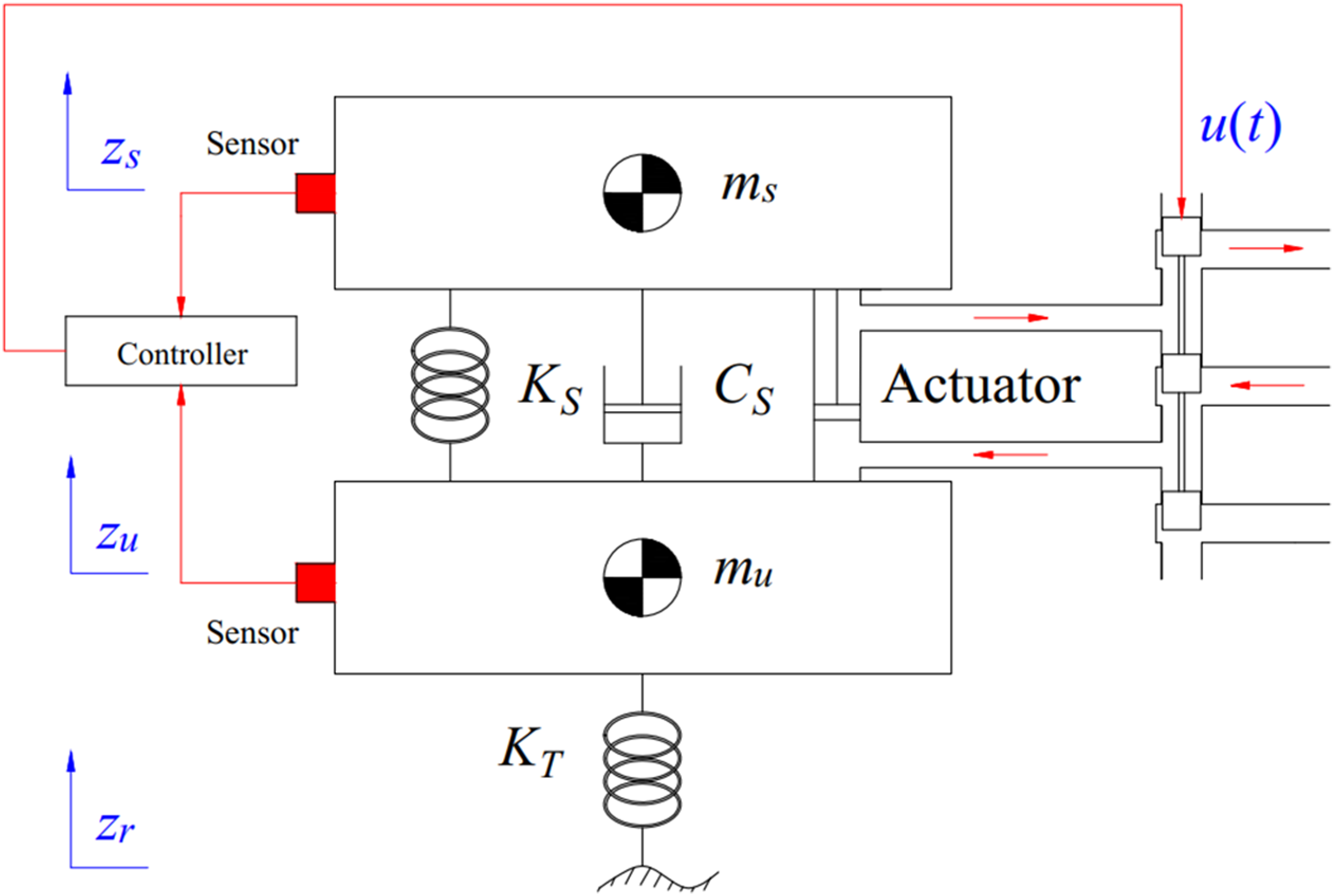

Applying D’Alembert’s principle to find the dynamic equations of the system, we get (1) and (2).

F_{i s} = F_{K S} + F_{C S} + F_{A S}

(1)

F_{i u} = F_{K T} - F_{K S} - F_{C S} - F_{A S}

(2)

The linking forces are determined according to equations (3)–(8), in which F_KS is the suspension spring force, F_CS is the suspension damping force, F_AS is the suspension actuator force, F_KT is the tire spring force, F_is is the inertia force of the sprung mass, F_iu is the inertia force of the unsprung mass, K_S is the stiffness of the suspension spring, C_S is the stiffness of the suspension damper, K_T is the stiffness of the tire spring, γ_i are coefficients of the hydraulic actuator, and u(t) is the control signal.

F_{K S} = K_{S} (z_{u} - z_{s})

(3)

F_{C S} = C_{S} ({\dot{z}}_{u} - {\dot{z}}_{s})

(4)

F_{K T} = K_{T} (z_{r} - z_{u})

(5)

{\dot{F}}_{A S} = γ_{1} u (t) - γ_{2} F_{A S} - γ_{3} ({\dot{z}}_{s} - {\dot{z}}_{u})

(6)

F_{i s} = m_{s} {\ddot{z}}_{s}

(7)

F_{i u} = m_{u} {\ddot{z}}_{u}

(8)

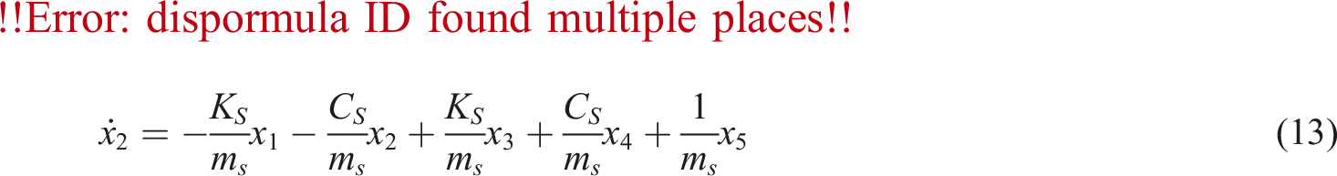
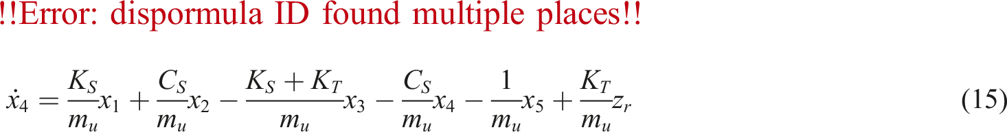
Substituting the linking equations into (1) and (2), we get (9) and (10).

m_{s} {\ddot{z}}_{s} = - K_{S} z_{s} - C_{S} {\dot{z}}_{s} + K_{S} z_{u} + C_{S} {\dot{z}}_{u} + F_{A S}

(9)

m_{u} {\ddot{z}}_{u} = K_{S} z_{s} + C_{S} {\dot{z}}_{s} - (K_{S} + K_{T}) z_{u} - C_{S} {\dot{z}}_{u} - F_{A S} + K_{T} z_{r}

(10)

Let the state variables be as mentioned in (11). Taking their derivatives, we obtain (12) to (16).

{[\begin{array}{l} x_{1} & x_{2} & x_{3} & x_{4} & x_{5} \end{array}]}^{T} = {[\begin{array}{l} z_{s} & {\dot{z}}_{s} & z_{u} & {\dot{z}}_{u} & F_{A} \end{array}]}^{T}

(11)

{\dot{x}}_{1} = x_{2}

(12)

{\dot{x}}_{2} = - \frac{K_{S}}{m_{s}} x_{1} - \frac{C_{S}}{m_{s}} x_{2} + \frac{K_{S}}{m_{s}} x_{3} + \frac{C_{S}}{m_{s}} x_{4} + \frac{1}{m_{s}} x_{5}

(13)

{\dot{x}}_{3} = x_{4}

(14)

{\dot{x}}_{4} = \frac{K_{S}}{m_{u}} x_{1} + \frac{C_{S}}{m_{u}} x_{2} - \frac{K_{S} + K_{T}}{m_{u}} x_{3} - \frac{C_{S}}{m_{u}} x_{4} - \frac{1}{m_{u}} x_{5} + \frac{K_{T}}{m_{u}} z_{r}

(15)

{\dot{x}}_{5} = - γ_{3} x_{2} + γ_{3} x_{4} - γ_{2} x_{5} + γ_{1} u (t)

(16)

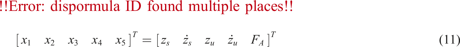
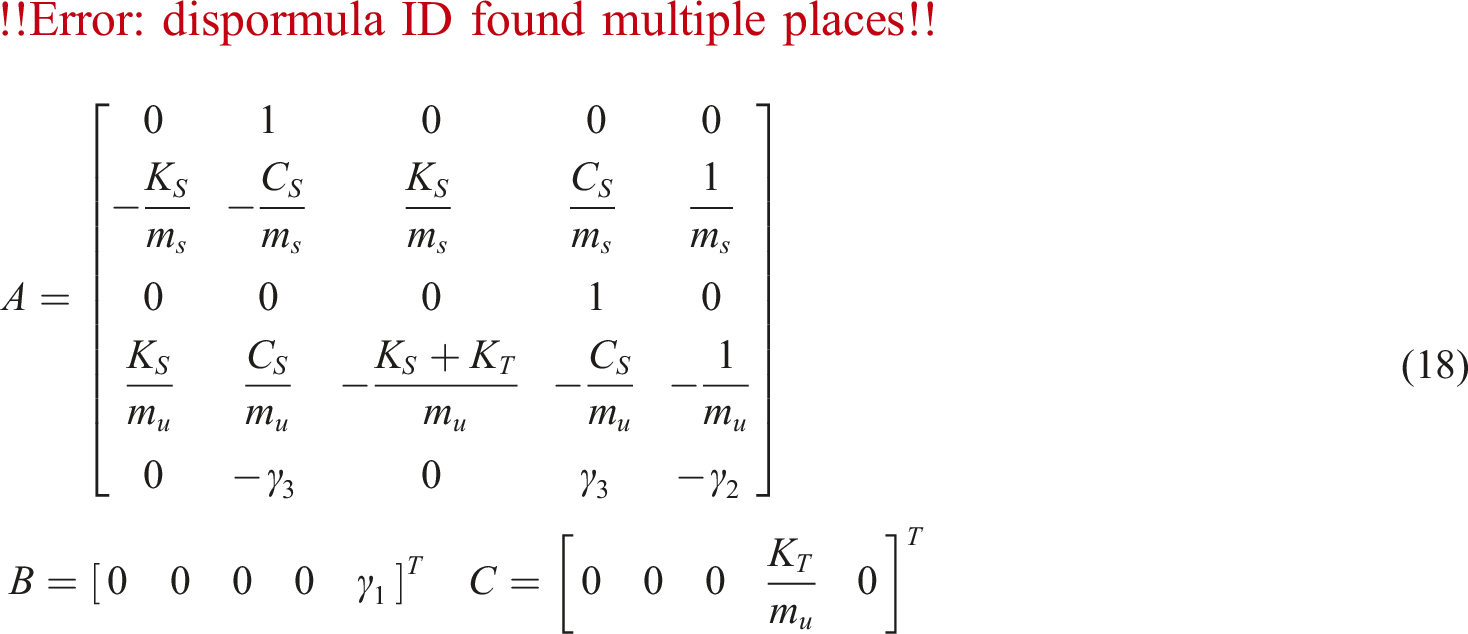
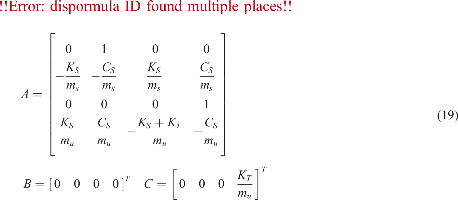
The automotive oscillation model is rewritten according to (17), which is established by equations from (11) to (16). The state matrices are determined according to (18) for the active suspension system and according to (19) for the passive suspension system.

[\dot{x}] = A [x] + B u (t) + C z_{r}

(17)

\begin{array}{l} A = [\begin{array}{c} 0 & 1 & 0 & 0 & 0 \\ - \frac{K_{S}}{m_{s}} & - \frac{C_{S}}{m_{s}} & \frac{K_{S}}{m_{s}} & \frac{C_{S}}{m_{s}} & \frac{1}{m_{s}} \\ 0 & 0 & 0 & 1 & 0 \\ \frac{K_{S}}{m_{u}} & \frac{C_{S}}{m_{u}} & - \frac{K_{S} + K_{T}}{m_{u}} & - \frac{C_{S}}{m_{u}} & - \frac{1}{m_{u}} \\ 0 & - γ_{3} & 0 & γ_{3} & - γ_{2} \end{array}] \\ \begin{array}{l} B = {[\begin{array}{l} 0 & 0 & 0 & 0 & γ_{1} \end{array}]}^{T} & C = {[\begin{array}{l} 0 & 0 & 0 & \frac{K_{T}}{m_{u}} & 0 \end{array}]}^{T} \end{array} \end{array}

(18)

\begin{array}{l} A = [\begin{array}{c} 0 & 1 & 0 & 0 \\ - \frac{K_{S}}{m_{s}} & - \frac{C_{S}}{m_{s}} & \frac{K_{S}}{m_{s}} & \frac{C_{S}}{m_{s}} \\ 0 & 0 & 0 & 1 \\ \frac{K_{S}}{m_{u}} & \frac{C_{S}}{m_{u}} & - \frac{K_{S} + K_{T}}{m_{u}} & - \frac{C_{S}}{m_{u}} \end{array}] \\ \begin{array}{l} B = {[\begin{array}{l} 0 & 0 & 0 & 0 \end{array}]}^{T} & C = {[\begin{array}{l} 0 & 0 & 0 & \frac{K_{T}}{m_{u}} \end{array}]}^{T} \end{array} \end{array}

(19)

Control model

In this article, we propose designing the hybrid control algorithm for the active suspension system. This algorithm is shaped by combining the ADRC and dynamic fuzzy techniques. The controlled object is the actuator force (x₅). The ADRC controller is formed based on the ESO and dual PID feedback control law.

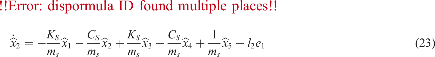
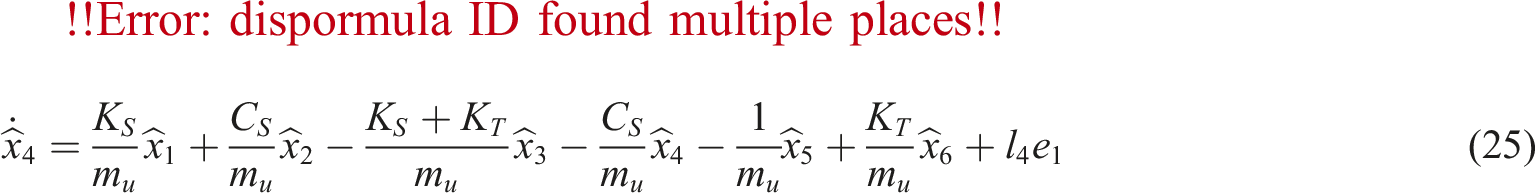
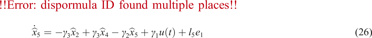
Assume that the sensor only measures the sprung mass displacement signal (x₁); the ESO estimates the remaining signals. Let the error between the measured and observed signals be e₁, as indicated by (20). According to (21), the system disturbance (z_r) is described through an augmented state variable (x₆). The remaining state variables are determined by integrating equations from (22) to (27), where l_i are gain parameters.

e_{1} = x_{1} - {\hat{x}}_{1}

(20)

{\hat{x}}_{6} = z_{r}

(21)

{\dot{\hat{x}}}_{1} = {\hat{x}}_{2} + l_{1} e_{1}

(22)

{\dot{\hat{x}}}_{2} = - \frac{K_{S}}{m_{s}} {\hat{x}}_{1} - \frac{C_{S}}{m_{s}} {\hat{x}}_{2} + \frac{K_{S}}{m_{s}} {\hat{x}}_{3} + \frac{C_{S}}{m_{s}} {\hat{x}}_{4} + \frac{1}{m_{s}} {\hat{x}}_{5} + l_{2} e_{1}

(23)

{\dot{\hat{x}}}_{3} = {\hat{x}}_{4} + l_{3} e_{1}

(24)

{\dot{\hat{x}}}_{4} = \frac{K_{S}}{m_{u}} {\hat{x}}_{1} + \frac{C_{S}}{m_{u}} {\hat{x}}_{2} - \frac{K_{S} + K_{T}}{m_{u}} {\hat{x}}_{3} - \frac{C_{S}}{m_{u}} {\hat{x}}_{4} - \frac{1}{m_{u}} {\hat{x}}_{5} + \frac{K_{T}}{m_{u}} {\hat{x}}_{6} + l_{4} e_{1}

(25)

{\dot{\hat{x}}}_{5} = - γ_{3} {\hat{x}}_{2} + γ_{3} {\hat{x}}_{4} - γ_{2} {\hat{x}}_{5} + γ_{1} u (t) + l_{5} e_{1}

(26)

{\dot{\hat{x}}}_{6} = l_{6} e_{1}

(27)

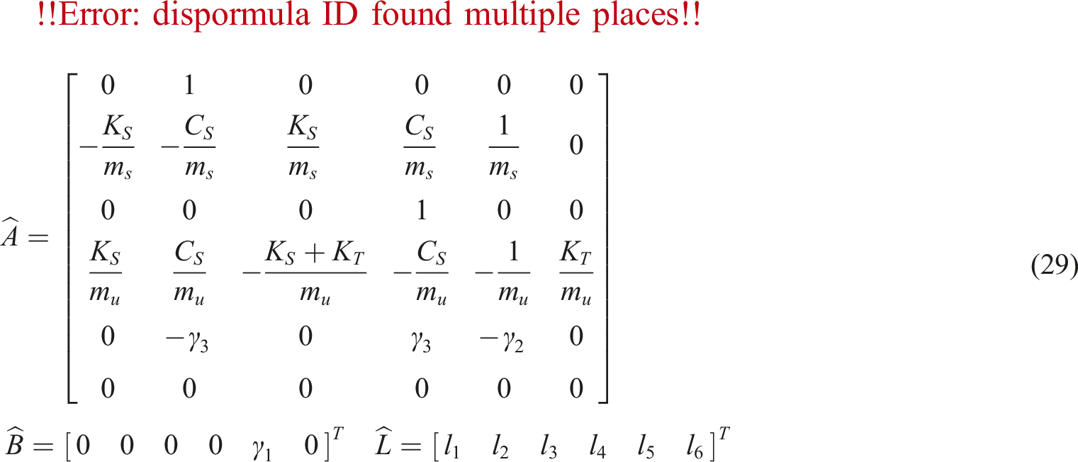
The above equations are rewritten concisely, according to (28). The expanded matrices are explained in (29).

[\dot{\hat{x}}] = \hat{A} [\hat{x}] + \hat{B} u (t) + \hat{L} e_{1}

(28)

\begin{array}{l} \hat{A} = [\begin{array}{c} 0 & 1 & 0 & 0 & 0 & 0 \\ - \frac{K_{S}}{m_{s}} & - \frac{C_{S}}{m_{s}} & \frac{K_{S}}{m_{s}} & \frac{C_{S}}{m_{s}} & \frac{1}{m_{s}} & 0 \\ 0 & 0 & 0 & 1 & 0 & 0 \\ \frac{K_{S}}{m_{u}} & \frac{C_{S}}{m_{u}} & - \frac{K_{S} + K_{T}}{m_{u}} & - \frac{C_{S}}{m_{u}} & - \frac{1}{m_{u}} & \frac{K_{T}}{m_{u}} \\ 0 & - γ_{3} & 0 & γ_{3} & - γ_{2} & 0 \\ 0 & 0 & 0 & 0 & 0 & 0 \end{array}] \\ \begin{array}{l} \hat{B} = {[\begin{array}{l} 0 & 0 & 0 & 0 & γ_{1} & 0 \end{array}]}^{T} & \hat{L} = {[\begin{array}{l} l_{1} & l_{2} & l_{3} & l_{4} & l_{5} & l_{6} \end{array}]}^{T} \end{array} \end{array}

(29)

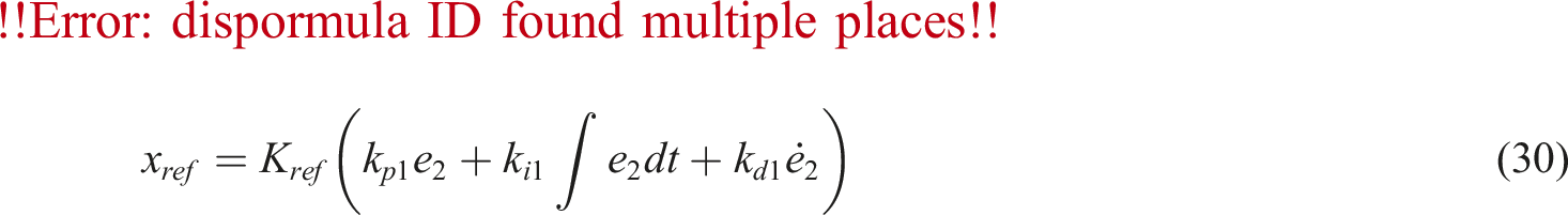
Previous research results show that the control force is in the opposite direction to the disturbance, and the value of the control force is much larger than the value of the disturbance^43,44 (*). Furthermore, the vehicle body’s displacement is in the same direction as the system disturbance^45–47 (**). Based on these comments, we propose to use a reference signal (x_ref) as the target control force, as shown in (30). As mentioned earlier (*), the control force and disturbance have similar variation, but their values differ due to their different units. Therefore, the reference signal (x_ref) can be generated by utilizing a PID algorithm to generate a desired signal based on the disturbance error (e₂), which is then amplified by a gain coefficient (K_ref). This ensures that the target control force (x_ref) tends to vary following the external disturbance, and its values are always guaranteed to be consistent. In this work, the disturbance error (e₂) is determined by the difference between the observed system disturbance and the observed vehicle body displacement, according to (31). This equation is consistent with the comment given above (**). A constant (K_e) is used in (31) to ensure the similarity between x₆ and x₁, that is, to reduce the steady-state error.

x_{r e f} = K_{r e f} (k_{p 1} e_{2} + k_{i 1} \int e_{2} d t + k_{d 1} {\dot{e}}_{2})

(30)

e_{2} = {\hat{x}}_{6} - K_{e} {\hat{x}}_{1}

(31)

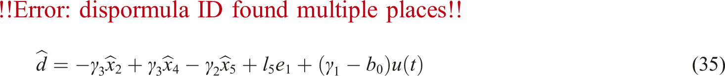
The control mechanism of ADRC is depicted in Figure 2. As per this description, the control signal (u(t)) is determined by (32). The initial control signal (u₀) is calculated based on a PID controller (33), where e₃ represents the error between the reference signal and the controlled signal, determined by (34). A comprehensive explanation of the system’s total disturbances is provided in (35), where b₀ denotes a critical gain. Using the ESO to determine the change of external disturbance and total disturbance provides several advantages. First, the system cost is significantly reduced because it is not necessary to use expensive physical sensors. Second, the influence of sensor noise is eliminated. Third, the influence of measurement error and delay is minimized, increasing the system’s processing speed. Finally, the total disturbance identification (35) helps eliminate adverse effects on the system, thus improving the controller’s performance.

u (t) = \frac{u_{0} - \hat{d}}{b_{0}}

(32)

u_{0} = k_{p 2} e_{3} + k_{i 2} \int e_{3} d t + k_{d 2} {\dot{e}}_{3}

(33)

e_{3} = x_{r e f} - {\hat{x}}_{5}

(34)

\hat{d} = - γ_{3} {\hat{x}}_{2} + γ_{3} {\hat{x}}_{4} - γ_{2} {\hat{x}}_{5} + l_{5} e_{1} + (γ_{1} - b_{0}) u (t)

(35)

Figure 2.

Control scheme.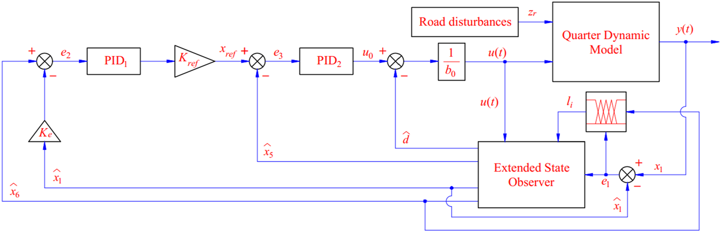

The choice of gain parameters (l_i) is essential because it determines the ESO’s performance. In reality, the road excitation (external disturbance) changes continuously over time and may not follow any rules. Therefore, the choice of fixed gain parameters may degrade the system’s performance in some cases, even if those parameters have been calculated optimally. In this article, we propose to design a dynamic fuzzy algorithm to tune l₁ and l₂ to improve the system’s adaptability.

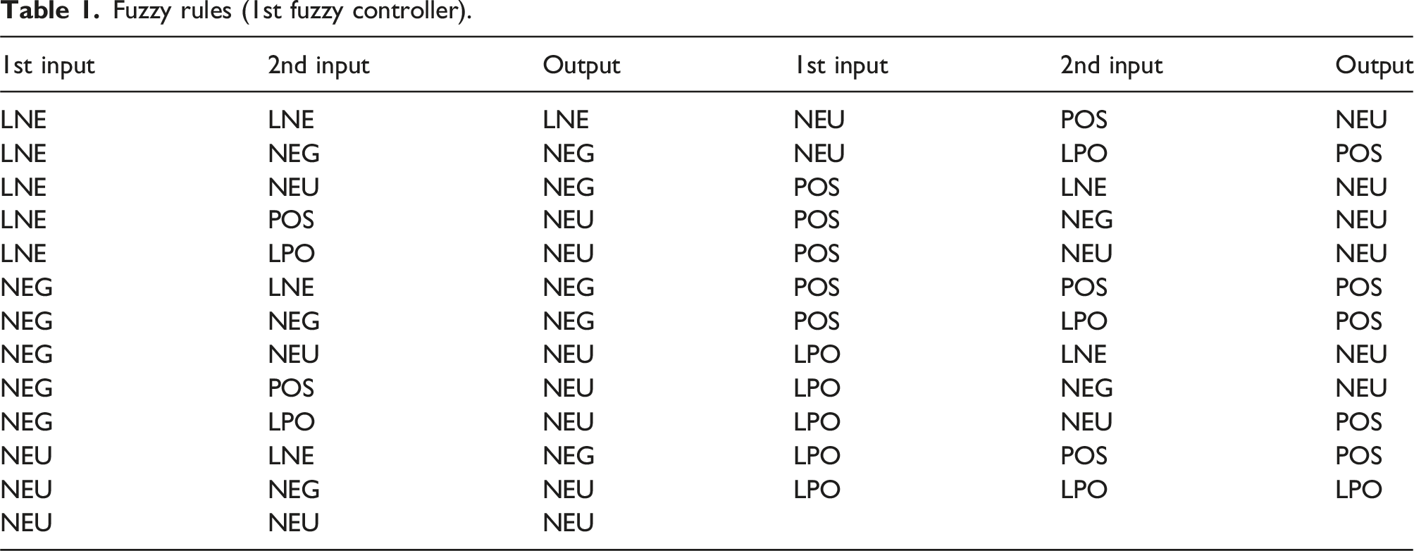
The first fuzzy controller is utilized to tune l₁. This controller is formed by two inputs and one output. The first input is the error between the measured and observed signals (e₁), while the other input is the observed road disturbances. The second fuzzy controller tunes l₂ and shares a structure with the first one. The second input, however, is the derivative of the road disturbance signal.

Figure 3(a) provides information about the membership functions utilized for the first fuzzy controller’s first input. This figure illustrates that the first input (e₁) undergoes fuzzification through triangular and trapezoidal functions. Triangular membership functions (TRIMFs) are employed for a small error range, while trapezoidal membership functions (TRAPMFs) determine membership degrees for larger error values. As for the second input, Gaussian membership functions (GAUSSMFs) replace the triangular functions (Figure 3(b)). The system considers five levels: Large Negative (LNE), Negative (NEG), Neutral (NEU), Positive (POS), and Large Positive (LPO). Equations (36) and (37) model the first input using TRIMFs and TRAPMFs, respectively. Regarding the second input, GAUSSMFs and TRAPMFs are represented by equations (38) and (39), respectively.

μ_{F 11} (e_{1}; a, b, c) = \max (\min (\frac{e_{1} - a}{b - a}, \frac{c - e_{1}}{c - b}), 0)

(36)

μ_{F 11} (e_{1}; a, b, c, d) = \max (\min (\frac{e_{1} - a}{b - a}, 1, \frac{d - e_{1}}{d - c}), 0)

(37)

μ_{F 12} ({\hat{x}}_{6}; σ, c) = e^{- \frac{{({\hat{x}}_{6} - c)}^{2}}{2 σ^{2}}}

(38)

μ_{F 12} ({\hat{x}}_{6}; a, b, c, d) = \max (\min (\frac{{\hat{x}}_{6} - a}{b - a}, 1, \frac{d - {\hat{x}}_{6}}{d - c}), 0)

(39)

Figure 3.

Membership functions: (a) the first input of 1st fuzzy controller, (b) the second input of 1st fuzzy controller, (c) the first input of 2nd fuzzy controller, and (d) the second input of 2nd fuzzy controller.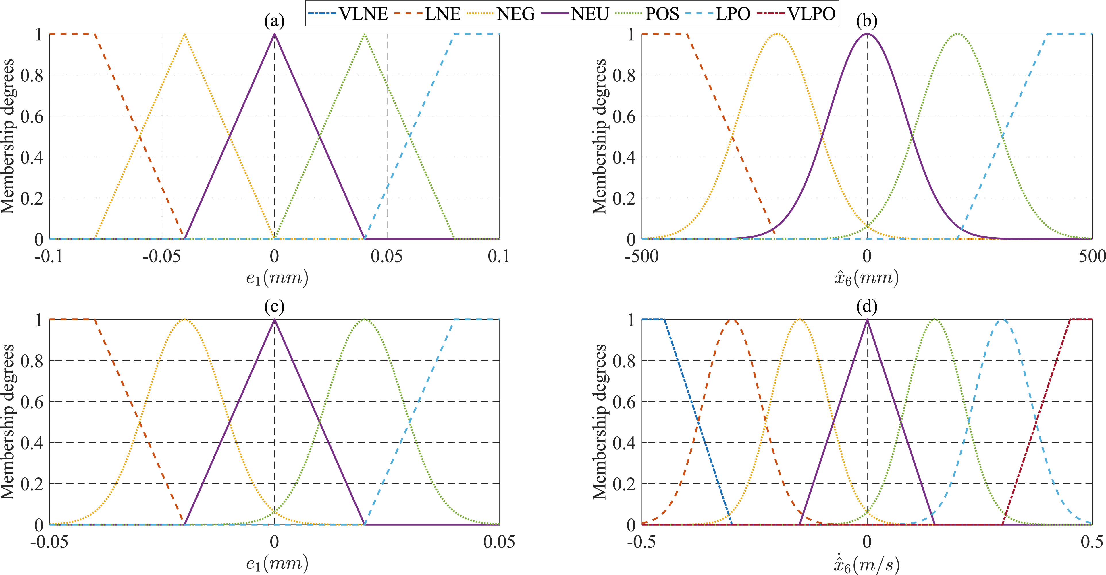

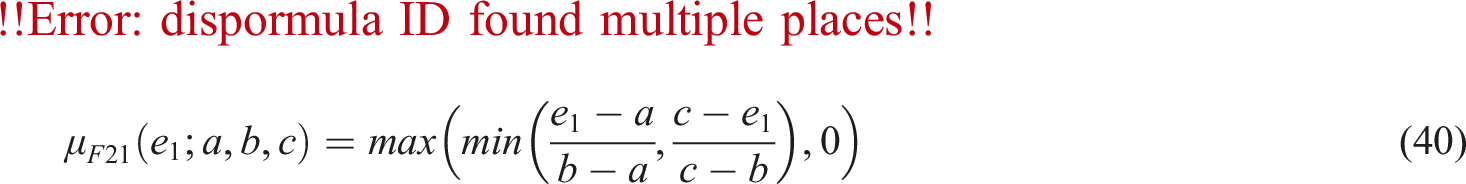
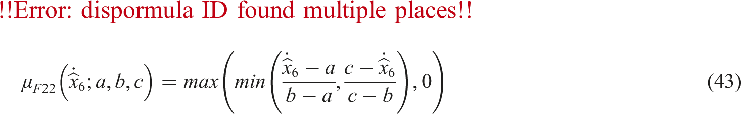
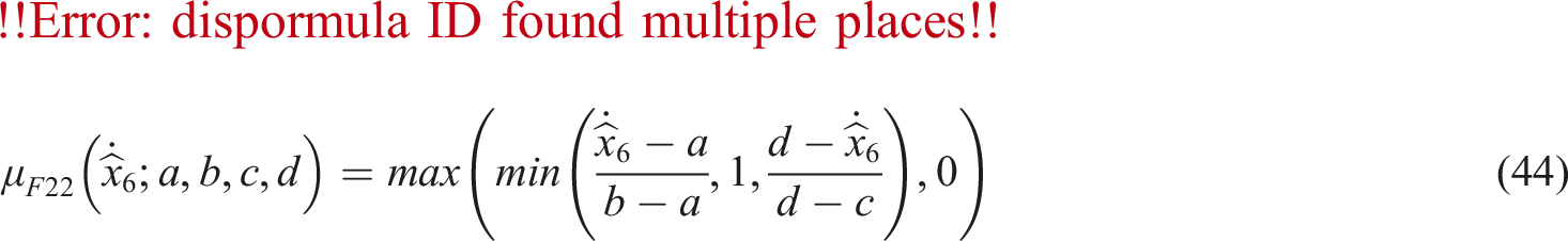
An improvement in membership functions is seen when GAUSSMFs are substituted for TRIMFs. A central TRIMF is still utilized to enhance the system’s response speed (Figure 3(c)). The number of MFs in Figure 3(d) is more substantial than previous figures, introducing two additional steps: Very Large Negative (VLNE) and Very Large Positive (VLPO). This adjustment aims to mitigate abrupt value changes when the disturbance speed varies. The structure of the membership functions mentioned in Figure 3(c) (the first input) is shown in equations from (40) to (42). Likewise, equations from (43) to (45) delineate the formulation of the MFs for the second input.

μ_{F 21} (e_{1}; a, b, c) = \max (\min (\frac{e_{1} - a}{b - a}, \frac{c - e_{1}}{c - b}), 0)

(40)

μ_{F 21} (e_{1}; a, b, c, d) = \max (\min (\frac{e_{1} - a}{b - a}, 1, \frac{d - e_{1}}{d - c}), 0)

(41)

μ_{F 21} (e_{1}; σ, c) = e^{- \frac{{(e_{1} - c)}^{2}}{2 σ^{2}}}

(42)

μ_{F 22} ({\dot{\hat{x}}}_{6}; a, b, c) = \max (\min (\frac{{\dot{\hat{x}}}_{6} - a}{b - a}, \frac{c - {\dot{\hat{x}}}_{6}}{c - b}), 0)

(43)

μ_{F 22} ({\dot{\hat{x}}}_{6}; a, b, c, d) = \max (\min (\frac{{\dot{\hat{x}}}_{6} - a}{b - a}, 1, \frac{d - {\dot{\hat{x}}}_{6}}{d - c}), 0)

(44)

μ_{F 22} ({\dot{\hat{x}}}_{6}; σ, c) = e^{- \frac{{({\dot{\hat{x}}}_{6} - c)}^{2}}{2 σ^{2}}}

(45)

Note: a, b, c, d, and σ are specific coefficients. It is noted that the coefficients mentioned in equations (36) to (45) are different.

The output of the fuzzy controller is calculated by the fuzzy rules, which are listed in Table 1 (1st fuzzy controller) and Table 2 (2nd fuzzy controller).

Table 1.

Fuzzy rules (1st fuzzy controller).

1st input	2nd input	Output	1st input	2nd input	Output
LNE	LNE	LNE	NEU	POS	NEU
LNE	NEG	NEG	NEU	LPO	POS
LNE	NEU	NEG	POS	LNE	NEU
LNE	POS	NEU	POS	NEG	NEU
LNE	LPO	NEU	POS	NEU	NEU
NEG	LNE	NEG	POS	POS	POS
NEG	NEG	NEG	POS	LPO	POS
NEG	NEU	NEU	LPO	LNE	NEU
NEG	POS	NEU	LPO	NEG	NEU
NEG	LPO	NEU	LPO	NEU	POS
NEU	LNE	NEG	LPO	POS	POS
NEU	NEG	NEU	LPO	LPO	LPO
NEU	NEU	NEU

Table 2.

Fuzzy rules (2nd fuzzy controller).

1st input	2nd input	Output	1st input	2nd input	Output	1st input	2nd input	Output
LNE	VLNE	VLNE	NEG	LPO	POS	POS	NEU	NEU
LNE	LNE	LNE	NEG	VLPO	LPO	POS	POS	POS
LNE	NEG	LNE	NEU	VLNE	NEG	POS	LPO	LPO
LNE	NEU	NEG	NEU	LNE	NEG	POS	VLPO	LPO
LNE	POS	NEG	NEU	NEG	NEU	LPO	VLNE	NEG
LNE	LPO	NEU	NEU	NEU	NEU	LPO	LNE	NEU
LNE	VLPO	POS	NEU	POS	NEU	LPO	NEG	POS
NEG	VLNE	LNE	NEU	LPO	POS	LPO	NEU	POS
NEG	LNE	LNE	NEU	VLPO	POS	LPO	POS	LPO
NEG	NEG	NEG	POS	VLNE	NEG	LPO	LPO	LPO
NEG	NEU	NEU	POS	LNE	NEG	LPO	VLPO	VLPO
NEG	POS	NEU	POS	NEG	NEU

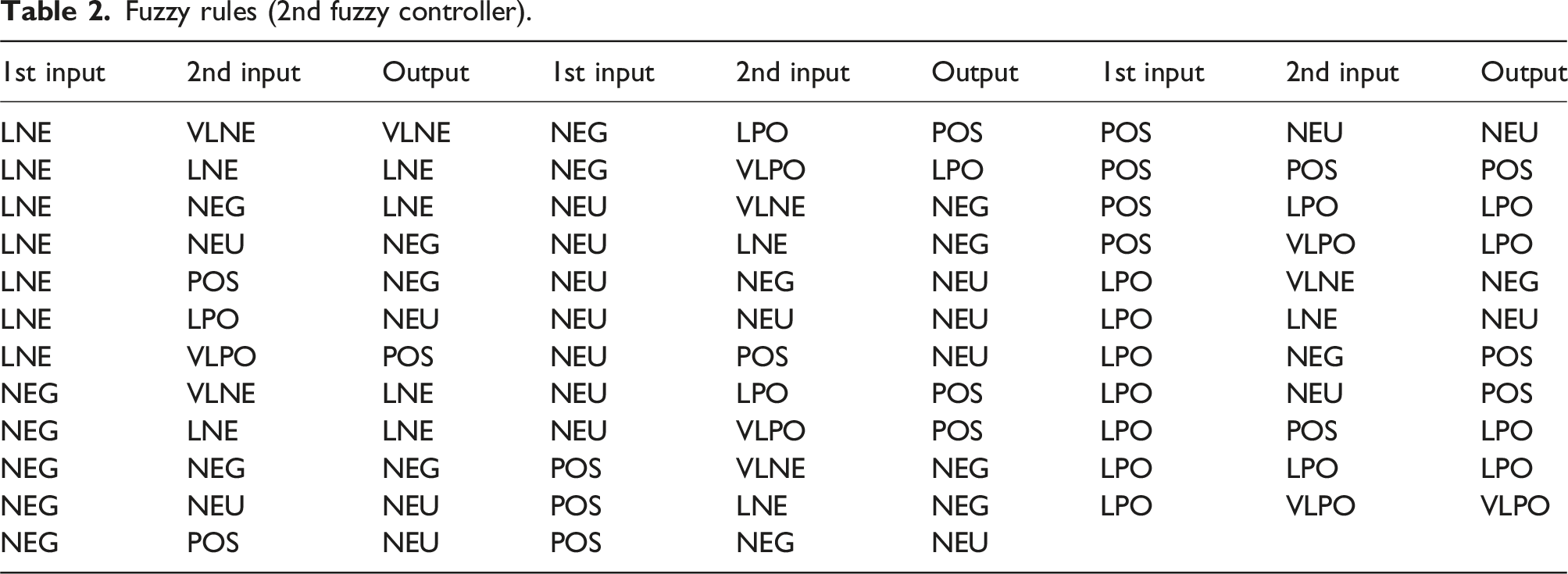
The relationship between the inputs and outputs of fuzzy controllers is illustrated by fuzzy surfaces (Figure 4). These surfaces are formed based on the MFs and fuzzy rules mentioned above.

Figure 4.

Fuzzy surfaces: (a) fuzzy surfaces for 1st controller and (b) fuzzy surfaces for 2nd controller.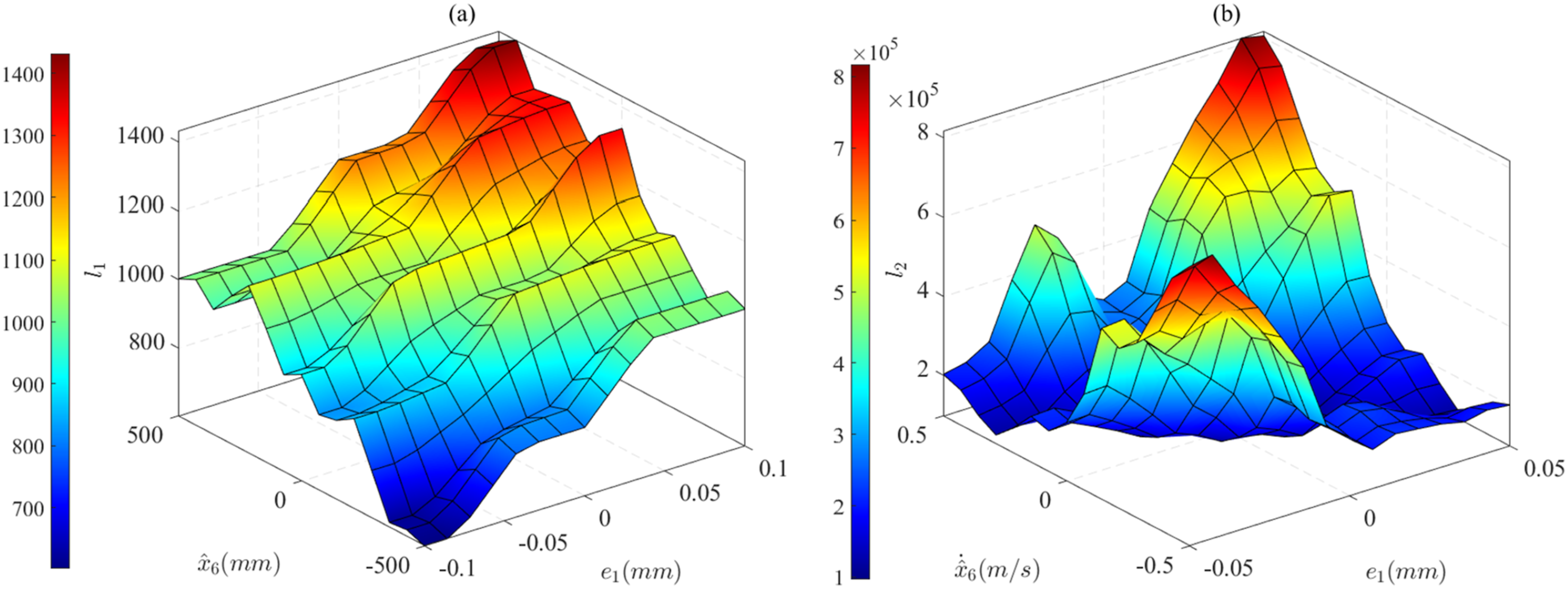

Simulation and discussion

Simulations are performed to validate the performance of the proposed algorithm. Road disturbances are the excitation sources causing vehicle vibrations (inputs to the problem), while the outputs include sprung mass displacement, sprung mass acceleration, and suspension travel. Three cases are investigated, corresponding to three types of road disturbances: sinusoidal excitation, step excitation, and trapezoidal excitation. The results obtained by the proposed algorithm (ADRCF) are compared with other control methods to demonstrate the algorithm’s effectiveness. The vehicle specifications are listed in Table 3, referenced from CARSIM and recalibrated to suit real-world conditions. The specifications of the actuator should be referred to in Ref. 44.

Table 3.

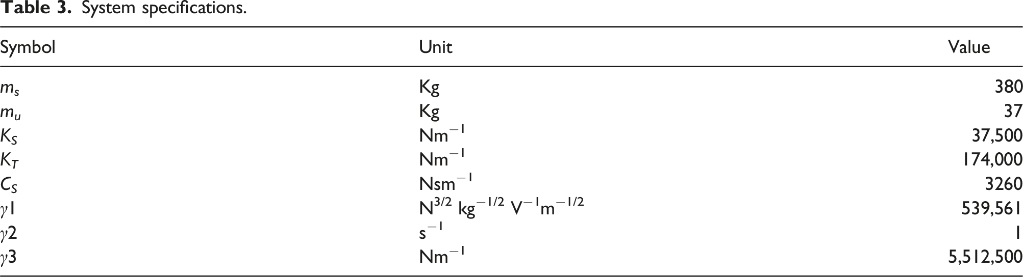
System specifications.

Symbol	Unit	Value
m _s	Kg	380
m _u	Kg	37
K _S	Nm⁻¹	37,500
K _T	Nm⁻¹	174,000
C _S	Nsm⁻¹	3260
γ1	N^3/2 kg^−1/2 V⁻¹m^−1/2	539,561
γ2	s⁻¹	1
γ3	Nm⁻¹	5,512,500

Sinusoidal excitation

The sinusoidal excitation is considered a road disturbance in the first case of investigation. The simulation results are illustrated by the subplots in Figure 5. Looking at Figure 5(a) more closely, one can see that the disturbance signal observed by the ESO (cyan dashed line) closely follows the actual disturbance signal (gray solid line). The simulation results show that the RMS error between the actual signal (measured by the sensor) and the signal estimated by the ESO is 0.406 mm, while the mean error is only −0.005 mm.

Figure 5.

The simulation results under sinusoidal excitation: (a) road disturbances, (b) sprung mass displacement, (c) sprung mass acceleration, and (d) suspension travel.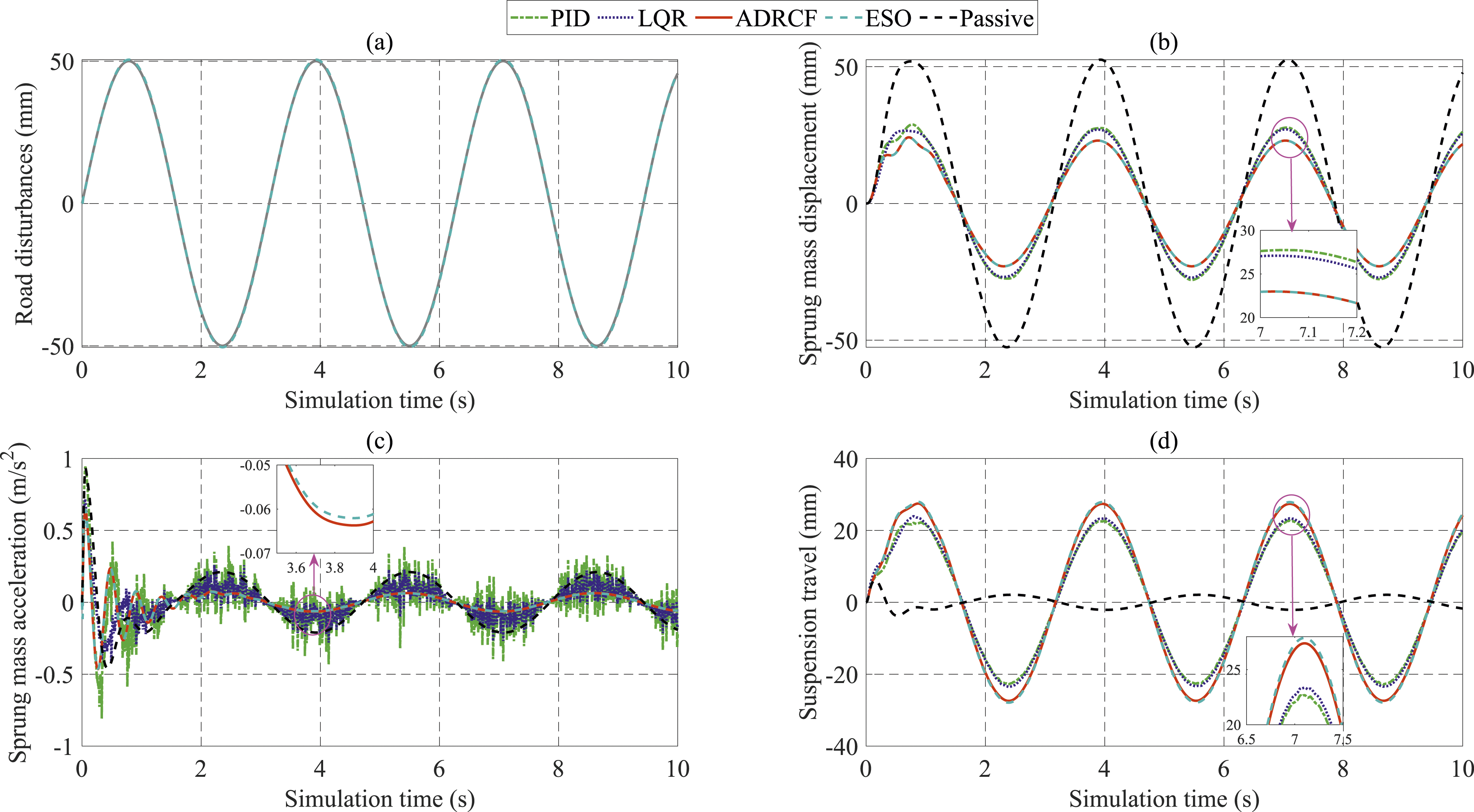

The variation of the sprung mass (vehicle body) displacement with time is illustrated in Figure 5(b). If the vehicle is equipped with only passive suspension, the vehicle body displacement can be as high as 52.576 mm. A significant degradation is seen when the passive suspension system is replaced by the active suspension system, which the conventional PID controller controls. The peak value of sprung mass displacement is reduced to 28.868 mm, slightly higher than that of LQR (27.142 mm). Once the proposed method (ADRCF) is applied to control the vehicle suspension system, the peak displacement of the vehicle body is only 24.178 mm, which is 0.001 mm higher than the value observed by the ESO. In terms of continuous vibration, the RMS value must be considered. According to the findings of the study, the RMS value of vehicle body displacement is 37.702 mm (Passive), 20.011 mm (PID), and 19.561 mm (LQR). The ADRCF algorithm provides superior performance compared to the conventional control methods, which causes the RMS value of vehicle body displacement to decrease sharply to 16.555 mm. The value observed by the ESO is approximately the actual value with zero error (after the result has been rounded). Furthermore, the proposed method almost eliminates the phase shift phenomenon.

Figure 5(c) shows the variation of the sprung mass acceleration over time. The peak acceleration of the vehicle body is 0.930 m/s² when the vehicle has only conventional passive suspension. This value increases to 0.943 m/s² when passive suspension is replaced by active suspension controlled by the traditional PID technique. The ride comfort is improved by applying the proposed control technique, which reduces the peak acceleration value to 0.646 m/s². The error obtained from the ESO compared to ADRCF is only 0.464%. The sensor noise phenomenon causes the acceleration to undergo continuous chattering. As a result, the RMS acceleration obtained from the PID controller is 0.175 m/s², which is 0.02 m/s² lower than that obtained from the passive suspension. In this case, the acceleration of the vehicle body obtained by the LQR controller is negatively affected by sensor noise, causing its RMS value to increase to 0.121 m/s². The result obtained by the ADRCF method is lower than that of the above control methods, causing the RMS acceleration to decrease to 0.101 m/s², which is close to the observed value.

The last subplot in Figure 5 depicts the change in suspension travel. Looking at Figure 5(d) more closely, we can see that the suspension system operates more vigorously when controlled by the ADRCF algorithm, causing the suspension travel to increase to 27.477 mm (peak value) and 19.600 mm (RMS value). The observed errors are 1.776% and 1.801%, respectively. The performance of the PID and LQR controllers is similar. As a result, the results obtained from the two conventional controllers are nearly identical. The passive suspension system performs much worse than the controlled suspension system.

Step excitation

A step excitation signal is utilized in the second case study. The profile of road disturbances is shown in Figure 6(a). The simulation results show that the maximum error between the actual and observed signals is approximately 2.5 mm (at the time of the sudden increase in the excitation pulse). Then, the error decreases to less than 0.5 mm. The displacement of the vehicle body is the largest when the vehicle has only passive suspension (73.598 mm), which is greater than the road disturbance. After reaching the peak, this value decreases to 50 mm, equivalent to the road disturbance (Figure 5(b)). The PID controller reduces the vehicle body displacement to 56.985 mm, which is 14.198 mm higher than the LQR. After that, the signal obtained from the PID and LQR controllers tends to decrease and remains the same with a slight difference. The ADRCF algorithm provides superior performance in reducing the vehicle body displacement, which reduces the value to 45.603 mm (peak value) and 22.347 mm (steady value). In this case, the error observed by the ESO is negligible.

Figure 6.

The simulation results under step excitation: (a) road disturbances, (b) sprung mass displacement, (c) sprung mass acceleration, and (d) suspension travel.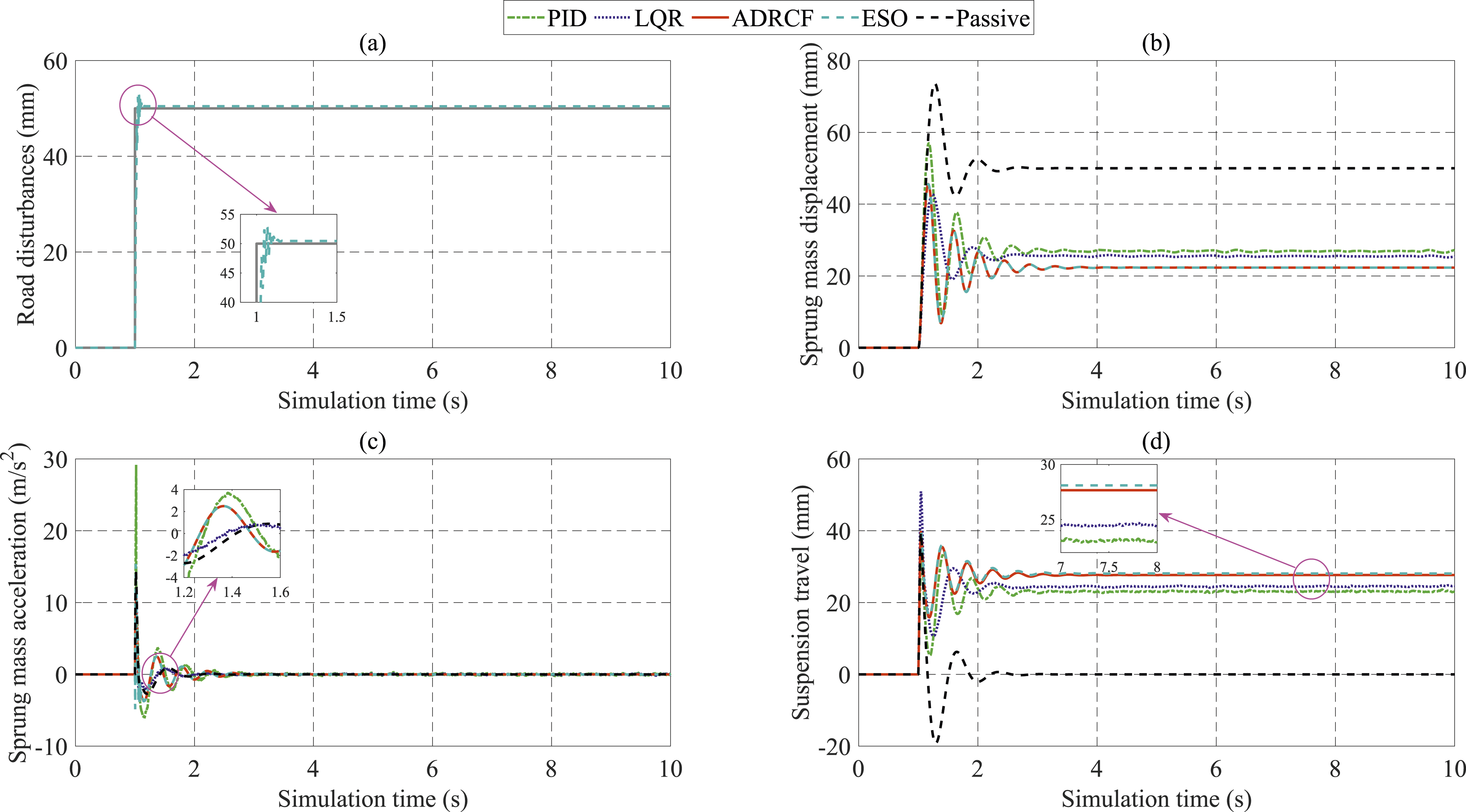

The vehicle body acceleration increases suddenly when applying the PID technique to control the suspension system (Figure 6(c)), up to 29.175 m/s². After that, this value gradually decreases to zero. The passive suspension system’s acceleration peaks at 14.338 m/s², 2.517 m/s² higher than the LQR control. The proposed algorithm’s control performance is superior to the two conventional control methods mentioned above. As a result, the peak value of the acceleration is only 10.583 m/s². In this case, the signal observed by the ESO has a significant error from the signal directly measured by the sensor, which is considered a limitation of the proposed algorithm.

Figure 6(d) presents suspension travel over time. Overall, the error between the observed signal and the value measured by the sensor is negligible (about 0.5 mm).

Trapezoidal pulse excitation

A trapezoidal pulse excitation is considered in the final case study. The ESO illustrates the profile of road disturbances (Figure 7(a)). The simulation results show that the observed error is small (less than 0.5 mm). The displacement of the vehicle body is significant when the vehicle only uses the conventional passive suspension system. The performance of the PID and LQR controllers is similar, reducing the displacement of the vehicle body by about half (Figure 7(b)). Compared with the two conventional control methods mentioned above, the ADRCF algorithm is more effective in reducing the sprung mass displacement based on its ability to adapt to various conditions. In this case, the vehicle body displacement observed by the ESO is close to the actual value with negligible error.

Figure 7.

The simulation results under trapezoidal pulse excitation: (a) road disturbances, (b) sprung mass displacement, (c) sprung mass acceleration, and (d) suspension travel.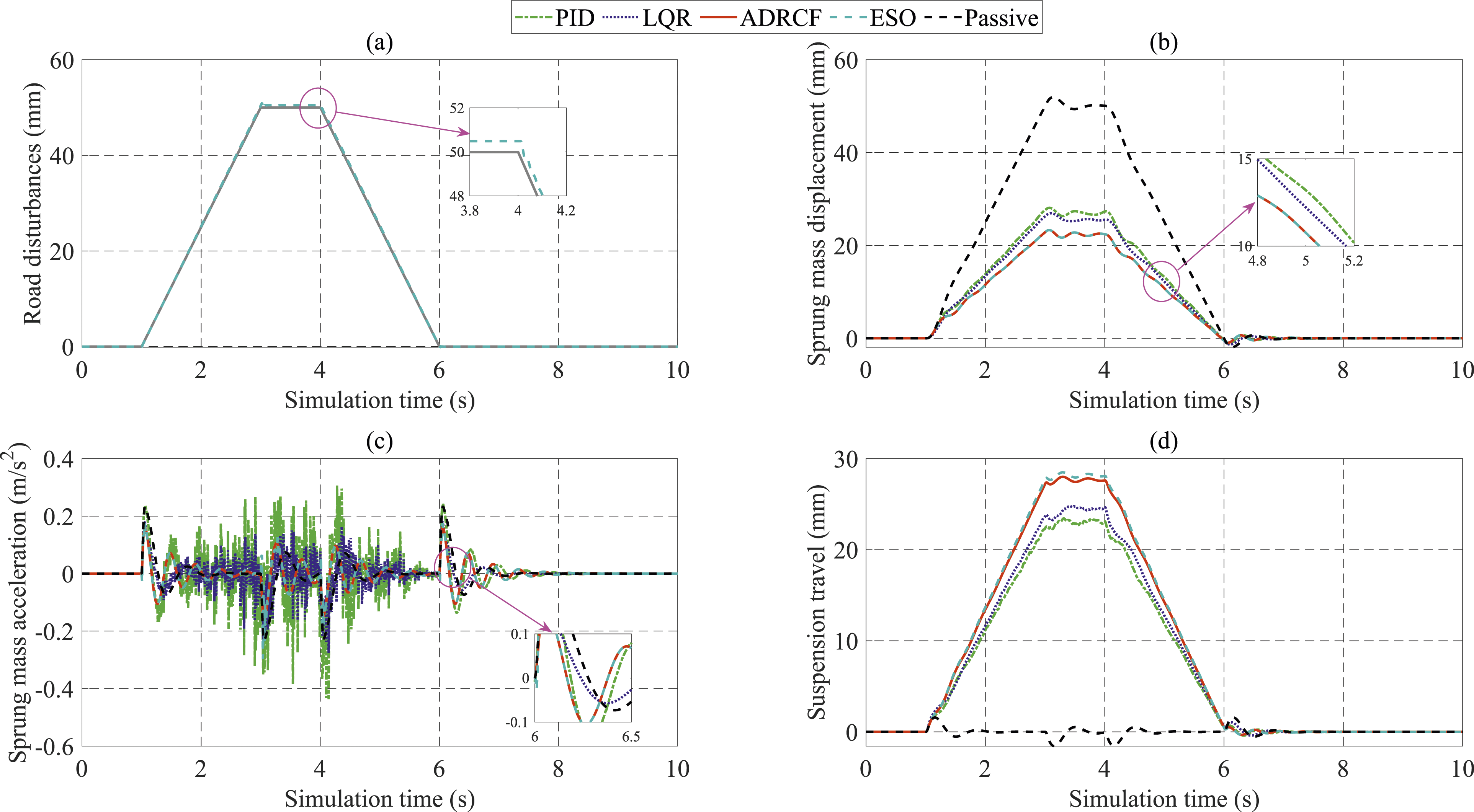

If the suspension system is controlled by PID and LQR controllers, the sprung mass acceleration will undergo intense chattering (Figure 7(c)). This is due to the phenomenon of sensor noise. In this article, we propose to use the ADRCF controller based on the ESO to estimate the change in the output state variables. The simulation results show that the proposed controller’s acceleration signal fluctuates more smoothly than the other two controllers.

Finally, the change in suspension travel is illustrated in Figure 7(d). According to this description, the suspension travel is the largest when the ADRCF algorithm controls the suspension system. At the same time, the performance of the PID and LQR controllers is only about 80% of that of the proposed algorithm. In this case, the observed error is less significant than 0.5 mm.

The simulation results above show that the displacement and acceleration of the vehicle body are reduced when the controllable active suspension system replaces the conventional passive suspension system. The values obtained by the proposed controller are superior to those of the PID and LQR controllers. The active suspension system needs to work harder to ensure that the acceleration and displacement are slight, that is, the suspension travel is increased compared to the passive suspension system. Finally, the results estimated by the ESO are highly accurate, which offers excellent potential in predicting the changes in values instead of having to measure them directly with expensive sensors. Overall, the ADRCF algorithm provides superior performance in suspension control, which overcomes some of the drawbacks of conventional control methods.

Conclusion

The active suspension system provides better comfort and smoothness than the conventional passive suspension system. The hybrid control algorithm is introduced in this article to control the performance of the automotive suspension system based on the reduction of vehicle body displacement. The proposed algorithm is formulated based on the ADRC technique, which was established by combining PID and ESO. The control parameters are tuned by dynamic fuzzy techniques to enhance the system’s adaptability.

The performance of the proposed algorithm is validated by simulation. According to the article’s findings, the vehicle body displacement is significantly reduced when the proposed technique is applied to control the suspension system, compared with the two traditional control techniques (PID and LQR). In addition, the observed signal tracks the actual signal with high accuracy. Additionally, the influence of sensor noise is significantly suppressed when the ADRCF method is applied.

Although the proposed algorithm performs better in controlling the system, it still has some limitations. First, the observed error is still significant in some moments when the vehicle body is subjected to sudden excitation. The reason for this is that the control parameters are not optimally selected. Second, uncertainties are not considered in the actuator’s dynamic model. Third, the vehicle dynamics model must be extended to consider the influence of roll and pitch angles. These are expected to be addressed in future works.

Footnotes

Declaration of conflicting interests

The author(s) declared no potential conflicts of interest with respect to the research, authorship, and/or publication of this article.

Funding

The author(s) received no financial support for the research, authorship, and/or publication of this article.

ORCID iD

Tuan Anh Nguyen

References

Nguyen

. The dynamic model and control algorithm for the active suspension system. Math Probl Eng 2023; 2023: 2889435. DOI: 10.1155/2023/2889435.

Wang

Zhao

Gong

, et al. Research on robust model predictive control for electro-hydraulic servo active suspension systems. IEEE Access 2018; 6: 3231–3240. DOI: 10.1109/access.2017.2787663.

Haemers

Derammelaere

Ionescu

C-M

, et al. Proportional-integral state-feedback controller optimization for a full-car active suspension setup using a genetic algorithm. IFAC-PapersOnLine 2018; 51(4): 1–6. DOI: 10.1016/j.ifacol.2018.06.004.

Gad

Metered

Bassiuny

, et al. Vibration control of MR-Damped half truck suspension system using proportional integral derivative controller tuned by ant colony optimization. SAE Technical Paper 2024; 1: 23. DOI: 10.4271/2024-01-2289.

Ab Talib

Mat Darus

Mohd Samin

, et al. Vibration control of semi-active suspension system using PID controller with advanced firefly algorithm and particle swarm optimization. J Ambient Intell Hum Comput 2020; 12(1): 1119–1137. DOI: 10.1007/s12652-020-02158-w.

Dahunsi

Dangor

Pedro

, et al. Proportional + integral + derivative control of nonlinear full-car electrohydraulic suspensions using global and evolutionary optimization techniques. J Low Freq Noise Vib Act Control 2019; 39(2): 393–415. DOI: 10.1177/1461348419842676.

Mahmoodabadi

Nejadkourki

. Optimal fuzzy adaptive robust PID control for an active suspension system. Aust J Mech Eng 2020; 20(3): 681–691. DOI: 10.1080/14484846.2020.1734154.

Aboelela

MAS

Hennas

RHM

. Development of a Fractional-Order PID controller using adaptive weighted PSO and genetic algorithms with applications. Amsterdam, Netherlands: Elsevier eBooks, 2018, pp. 511–551. DOI: 10.1016/b978-0-12-816152-4.00017-0.

Swethamarai

Lakshmi

. Adaptive-fuzzy fractional order PID controller-based active suspension for vibration control. IETE J Res 2020; 68(5): 3487–3502. DOI: 10.1080/03772063.2020.1768906.

10.

Shi

. Adaptive endocrine PID control for active suspension based on reinforcement learning. Proc Inst Mech Eng - Part D J Automob Eng 2024; 2024: 09544070241262354. DOI: 10.1177/09544070241262354.

11.

Liu

As’arry

Ahmed

, et al. Online optimal tuning of fuzzy PID controller using grey wolf optimizer for quarter car semi-active suspension system. Adv Mech Eng 2024; 16(2): 16878132231219620. DOI: 10.1177/16878132231219620.

12.

Nguyen

Dang

, et al. LQR control with the new triple in-loops algorithm for optimization of the tuning parameters. Mathe Model and Eng Prob 2022; 9(3): 628–636. DOI: 10.18280/mmep.090309.

13.

Das

Elumalai

Ganapathy Subramanian

, et al. Adaptive predator–prey optimization for tuning of infinite horizon LQR applied to vehicle suspension system. Appl Soft Comput 2018; 72: 518–526. DOI: 10.1016/j.asoc.2018.06.044.

14.

Başak

. Hybrid coati–grey wolf optimization with application to tuning linear quadratic regulator controller of active suspension systems. Eng Sci and Techan International J 2024; 56: 101765. DOI: 10.1016/j.jestch.2024.101765.

15.

Nagarkar

Bhalerao

Patil

, et al. Multi-objective optimization of nonlinear quarter car suspension system – PID and LQR control. Procedia Manuf 2018; 20: 420–427. DOI: 10.1016/j.promfg.2018.02.061.

16.

Bai

Wang

H-B

. Robust optimal control for the vehicle suspension system with uncertainties. IEEE Trans Cybern 2022; 52(9): 9263–9273. DOI: 10.1109/tcyb.2021.3052816.

17.

Jing

Wang

, et al. Robust finite-frequency H control of full-car active suspension. J Sound Vib 2019; 441: 221–239. DOI: 10.1016/j.jsv.2018.06.047.

18.

Wang

Jing

Karimi

, et al. Robust fault-tolerant H_∞ control of active suspension systems with finite-frequency constraint. Mech Syst Signal Process 2015; 62–63: 341–355. DOI: 10.1016/j.ymssp.2015.01.015.

19.

Chen

Yin

, et al. Robust H_∞ control design of an electromagnetic actuated active suspension considering the structure non-linearity. Proc Inst Mech Eng - Part D J Automob Eng 2018; 233(4): 1008–1022. DOI: 10.1177/0954407017753231.

20.

Afshar

Korzeniowski

Konieczny

. Constrained dynamic output-feedback robust H_∞ control of active inerter-based half-car suspension system with parameter uncertainties. IEEE Access 2023; 11: 46051–46072. DOI: 10.1109/access.2023.3272328.

21.

Pang

Zhang

Chen

, et al. Design of a coordinated adaptive backstepping tracking control for nonlinear uncertain active suspension system. Appl Math Model 2019; 76: 479–494. DOI: 10.1016/j.apm.2019.06.030.

22.

Sun

, et al. Fuzzy adaptive backstepping control for a class of active suspension systems. IFAC-PapersOnLine 2018; 51(31): 136–141. DOI: 10.1016/j.ifacol.2018.10.025.

23.

Pang

Zhang

. Adaptive backstepping-based tracking control design for nonlinear active suspension system with parameter uncertainties and safety constraints. ISA Trans 2019; 88: 23–36. DOI: 10.1016/j.isatra.2018.11.047.

24.

Homayoun

Arefi

Vafamand

, et al. Neural minimal learning backstepping control of stochastic active suspension systems with hydraulic actuator saturation. J Franklin Inst 2020; 357(18): 13687–13706. DOI: 10.1016/j.jfranklin.2020.10.020.

25.

Nguyen

. Advance the efficiency of an active suspension system by the sliding mode control algorithm with five state variables. IEEE Access 2021; 9: 164368–164378. DOI: 10.1109/access.2021.3134990.

26.

Arslan

Sezgin

Yagiz

. Improving the ride comfort of vehicle passenger using fuzzy sliding mode controller. J Vib Control 2013; 21(9): 1667–1679. DOI: 10.1177/1077546313500061.

27.

Xue

Yang

, et al. A hybrid sliding mode controller design for vibration suppression in a hydraulic suspension system with vertical load disturbance. J Vib Control 2022; 30(1–2): 377–391. DOI: 10.1177/10775463221147337.

28.

Pang

Shang

Wang

. Design of a sliding mode observer-based fault tolerant controller for automobile active suspensions with parameter uncertainties and sensor faults. IEEE Access 2020; 8: 186963–186975. DOI: 10.1109/access.2020.3029815.

29.

Nguyen

. A novel hybrid control algorithm sliding mode-PID for the active suspension system with state multivariable. Complexity 2022; 2022: 9527384. DOI: 10.1155/2022/9527384.

30.

Nguyen

Dang

. A novel sliding mode control algorithm for an active suspension system considering with the hydraulic actuator. Lat Am J Solid Struct 2022; 19(1): 78256883. DOI: 10.1590/1679-78256883.

31.

Ovalle

Ríos

Ahmed

. Robust control for an active suspension system via continuous sliding-mode controllers. Engineering Science and Technology an International Journal 2022; 28: 101026. DOI: 10.1016/j.jestch.2021.06.006.

32.

Abdul Zahra

Abdalla

. Design of fuzzy super twisting sliding mode control scheme for unknown full vehicle active suspension systems using an artificial bee colony optimization algorithm. Asian J Control 2020; 23(4): 1966–1981. DOI: 10.1002/asjc.2352.

33.

Nguyen

. Evaluate the stability of the vehicle when using the active suspension system with a hydraulic actuator controlled by the OSMC algorithm. Sci Rep 2022; 12: 19364. DOI: 10.1038/s41598-022-24069-w.

34.

Wijaya

Yakub

Abdullah

, et al. Adaptive estimation and control of nonlinear suspension systems with natural logarithm sliding mode control. IEEE Access 2024; 12: 60896–60907. DOI: 10.1109/access.2024.3393970.

35.

Wang

Chadli

Basin

. Practical terminal sliding mode control of nonlinear uncertain active suspension systems with adaptive disturbance observer. IEEE ASME Trans Mechatron 2021; 26(2): 789–797. DOI: 10.1109/tmech.2020.3000122.

36.

Fareh

Khadraoui

Abdallah

, et al. Active disturbance rejection control for robotic systems: a review. Mechatronics 2021; 80: 102671. DOI: 10.1016/j.mechatronics.2021.102671.

37.

Xiang

Guo

Wong

. Active disturbance rejection control of test sample in electrostatic suspension system. Mech Syst Signal Process 2021; 148: 107187. DOI: 10.1016/j.ymssp.2020.107187.

38.

Guo

Chen

. Active disturbance rejection control for electric power steering system with assist motor variable mode. J Franklin Inst 2018; 355(3): 1139–1155. DOI: 10.1016/j.jfranklin.2017.12.024.

39.

Zhang

. The effect of ADRC on vehicle braking performance. J Electr Eng Technol 2020; 15(2): 705–712. DOI: 10.1007/s42835-019-00340-5.

40.

Lam

Cheung

. Experimental investigation of active disturbance rejection control for vehicle suspension design. Int J Theor Appl Mech 2016; 1: 89–96.

41.

Lam

Cheung

. Motion-based active disturbance rejection control for a non-linear full-car suspension system. Proc Inst Mech Eng - Part D J Automob Eng 2017; 232(5): 616–631. DOI: 10.1177/0954407017704781.

42.

Muhammed

Yazan

Gavrilov

. Reference governed ADRC approach to manage the handling-comfort contradiction in a full-vehicle suspension. Trans Inst Meas Control 2022; 44(14): 2693–2708. DOI: 10.1177/01423312221089715.

43.

Nguyen

Tran

TTH

Hoang

. Design a new algorithm (iL-GA) to optimize controller parameters for an automotive suspension system. World Journal of Engineering. 2024. DOI: 10.1108/wje-10-2023-0444.

44.

Nguyen

. Proposing an original control algorithm for the active suspension system to improve vehicle vibration: adaptive fuzzy sliding mode proportional-integral-derivative tuned by the fuzzy (AFSPIDF). Heliyon 2023; 9(3): e14210. DOI: 10.1016/j.heliyon.2023.e14210.

45.

Nguyen

Iqbal

Tran

TTH

, et al. Application of hybrid control algorithm on the vehicle active suspension system to reduce vibrations. Adv Mech Eng 2024; 16(3): 16878132241239816. DOI: 10.1177/16878132241239816.

46.

Tran

Ahn

. Adaptive sliding mode control based nonlinear disturbance observer for active suspension with pneumatic spring. J Sound Vib 2021; 509: 116241. DOI: 10.1016/j.jsv.2021.116241.

47.

Gad

Metered

Bassuiny

, et al. Multi-objective genetic algorithm fractional-order PID controller for semi-active magnetorheologically damped seat suspension. J Vib Control 2015; 23(8): 1248–1266. DOI: 10.1177/1077546315591620.

1st input	2nd input	Output	1st input	2nd input	Output
LNE	LNE	LNE	NEU	POS	NEU
LNE	NEG	NEG	NEU	LPO	POS
LNE	NEU	NEG	POS	LNE	NEU
LNE	POS	NEU	POS	NEG	NEU
LNE	LPO	NEU	POS	NEU	NEU
NEG	LNE	NEG	POS	POS	POS
NEG	NEG	NEG	POS	LPO	POS
NEG	NEU	NEU	LPO	LNE	NEU
NEG	POS	NEU	LPO	NEG	NEU
NEG	LPO	NEU	LPO	NEU	POS
NEU	LNE	NEG	LPO	POS	POS
NEU	NEG	NEU	LPO	LPO	LPO
NEU	NEU	NEU

1st input	2nd input	Output	1st input	2nd input	Output
LNE	LNE	LNE	NEU	POS	NEU
LNE	NEG	NEG	NEU	LPO	POS
LNE	NEU	NEG	POS	LNE	NEU
LNE	POS	NEU	POS	NEG	NEU
LNE	LPO	NEU	POS	NEU	NEU
NEG	LNE	NEG	POS	POS	POS
NEG	NEG	NEG	POS	LPO	POS
NEG	NEU	NEU	LPO	LNE	NEU
NEG	POS	NEU	LPO	NEG	NEU
NEG	LPO	NEU	LPO	NEU	POS
NEU	LNE	NEG	LPO	POS	POS
NEU	NEG	NEU	LPO	LPO	LPO
NEU	NEU	NEU

Active disturbance rejection control for reducing vehicle body displacement based on an extended state observer and dynamic fuzzy techniques

Abstract

Keywords

Introduction

Literature review

Research gaps and new contributions

Mathematical method

Suspension model

Control model

Simulation and discussion

Sinusoidal excitation

Step excitation

Trapezoidal pulse excitation

Conclusion

Footnotes

Declaration of conflicting interests

Funding

ORCID iD

References

1st input	2nd input	Output	1st input	2nd input	Output
LNE	LNE	LNE	NEU	POS	NEU
LNE	NEG	NEG	NEU	LPO	POS
LNE	NEU	NEG	POS	LNE	NEU
LNE	POS	NEU	POS	NEG	NEU
LNE	LPO	NEU	POS	NEU	NEU
NEG	LNE	NEG	POS	POS	POS
NEG	NEG	NEG	POS	LPO	POS
NEG	NEU	NEU	LPO	LNE	NEU
NEG	POS	NEU	LPO	NEG	NEU
NEG	LPO	NEU	LPO	NEU	POS
NEU	LNE	NEG	LPO	POS	POS
NEU	NEG	NEU	LPO	LPO	LPO
NEU	NEU	NEU