
Abstract
Due to the uncertainty in vehicle model parameters, the control performance of active suspensions often deteriorates, especially under extreme conditions such as high velocities and full loads. To address this challenge, this paper proposes a novel robust finite frequency H ∞ output feedback control strategy based on linear parameter varying (LPV) systems. First, we establish a new LPV model for the half-car active suspension control system, taking into account the uncertainties associated with vehicle velocity and sprung mass. Next, a robust finite frequency H ∞ output feedback controller is designed using a gain scheduling approach, formulated through a set of linear matrix inequalities (LMIs). Finally, simulation results demonstrate that the proposed velocity-dependent robust control strategy significantly reduces the root mean square (RMS) values of vertical acceleration by approximately 21% to 31% under various conditions of sprung mass and vehicle speed compared to traditional control methods.
Introduction
The suspension system is an essential component of a vehicle, serving not only to support the vehicle’s weight but also to dampen body vibrations. In automotive research, suspension control remains a common topic of investigation. Depending on the implementation of control, suspension systems are classified as passive, semi-active, or active. 1 Active suspensions are more frequently utilized than passive suspensions in vehicle comfort studies because of their ease of implementation, rapid change in control force, and controlled performance. 2 However, the active suspension control force has a distinct saturation limit, and the damping force can only be continuously varied within a limited range, making the control strategy extremely important to the performance of the active suspension system. 3 Linear Quadratic Regulator (LQR) control, Model Predictive Control (MPC), and PID control are the three most commonly used control strategies.4–7
Traditional active cab suspension systems are often designed under the assumption that system parameters remain constant, such as vehicle speed, mass, stiffness, and damping. These systems are typically designed using Linear Time-Invariant (LTI) models, which have demonstrated commendable control performance compared to passive suspension systems. For instance, Nguyen 8 utilized a multi-loop algorithm to select optimal control parameters for sliding mode control under various vehicle vibration conditions, resulting in a significant reduction in body acceleration and displacement. Basaran 9 modeled a commercial vehicle cab suspension system based on a half-car model and proposes a design method utilizing Lyapunov backstepping control. Hamza 10 introduced a boundary model for Continuous Damping Control (CDC) dampers and develops an intelligent control method based on Artificial Neural Networks (ANN) for active truck suspension systems. However, these approaches encounter limitations in specific application scenarios where vehicle parameters fluctuate. To enhance the control performance of these systems, this study introduces Linear Parameter-Varying (LPV) control theory, which is better equipped to manage variability in vehicle parameters and improve the adaptability of the suspension system under diverse operating conditions. Since Shamma introduced LPV control theory, 11 it has become an important tool for addressing nonlinear system problems. The core of LPV control theory lay in approximating nonlinear systems as a set of parameter-dependent linear systems, allowing designers to utilize a variety of control methods from LTI systems to solve nonlinear control problems. Current research on LPV system control mainly focuses on three approaches: Linear Fractional Transformation (LFT), polytopic methods, and grid-based methods. The polytopic design approach has become a mainstream direction in the study of LPV systems due to its intuitive structure and the high degree of freedom it offers in controller design. 12 This method represents the system’s coefficient matrices in a polynomial or affine form. Tian 13 and Peng 14 studied path tracking and time-varying tire cornering stiffness uncertainties in autonomous vehicles based on LPV’s MPC and H ∞ gain-scheduled robust control strategies, significantly reducing computational complexity by simplifying the polytopic vertices.
In the design of vehicle suspension control systems, finite-frequency control strategies have gained attention due to their focus on vibration suppression within a specific frequency range. These strategies leverage the Kalman–Yakubovich–Popov (KYP) lemma to ingeniously transform performance and stability requirements in the frequency domain into time-domain conditions, which have been widely applied in filter design and control systems.15–17 According to the ISO-2631 standard, humans are most sensitive to vertical vibrations in the 4–8 Hz range, prompting researchers to apply finite-frequency control strategies to vehicle suspension systems to significantly enhance ride comfort. Sun 18 conducted in-depth research on finite-frequency control strategies. They applied the KYP lemma to optimize the H ∞ performance for the transfer function of road disturbances and control outputs in the 4–8 Hz frequency range, while also considering the time-domain constraints of actuator control force and suspension travel. Wang 19 designed a robust fault-tolerant H ∞ output feedback controller for a full-vehicle active suspension system with finite-frequency constraints using LFT to process uncertain parameter matrices, offering a new solution for the reliability of the suspension system. Jing 20 further developed a robust H ∞ state feedback controller based on uncertainties in suspension stiffness, damping, and tire stiffness, enhancing the system’s adaptability to parameter changes. Jiang, 21 in response to more complex uncertain conditions such as polyhedral uncertainty, external disturbances, state and input delays, and gain disturbances, proposed a non-fragile robust MPC strategy with delayed state compensation, providing ample design conditions for dealing with unobservable time-varying parameters in LPV systems.
During vehicle operation, the velocity is inherently variable, and the vehicle’s sprung mass is uncertain, varying with different loading conditions. These changes in vehicle model parameters can significantly affect ride comfort. Tsampardoukas 22 analyzed the impact mechanisms of key parameters on system performance under different road input conditions using a half-car model. Abdelkareem 23 further quantified the combined effects of vehicle velocity, damping coefficient, and road input on ride comfort, road adhesion, and damper energy dissipation. The existing research on suspension control strategies indicates that in practical scenarios, vehicle mass and speed are variable parameters. These fluctuations can cause the suspension control system to deviate from its preset optimal state, reducing vibration isolation performance, especially under complex road conditions. While it is possible to design control gains for each set of fixed parameters, this approach is only practical for situations with limited parameter variations. Designing and storing control gains for all possible parameter variations, particularly when there are significant changes in vehicle mass and speed, is clearly impractical. Therefore, drawing on valuable insights from existing LPV control and finite frequency H ∞ control theories to devise an integrated control method that can handle dynamic parameter variations and enhance control accuracy is a key technical issue in the research on active suspension control strategies for vehicles
To enhance ride comfort in the presence of vehicle velocity and sprung mass uncertainties, this paper presents two primary research contributions: 1. The introduction of a novel half-car LPV system model, which is parameterized by real-time vehicle speed. This model dynamically adjusts control gains in response to variations in vehicle speed, effectively mitigating the adverse effects of speed fluctuations on vibration attenuation. 2. The development of a robust finite frequency output feedback H
∞
control strategy, aimed at suppressing vibrations within the frequency band critical to human comfort perception. This strategy is designed to be resilient against uncertainties in sprung mass, ensuring consistent performance across a range of vehicle load conditions.
Problem formulation
In previous research,24–27 numerous complex suspension models have been proposed to simulate the dynamic properties of suspension systems. This paper employs a 4-degree-of-freedom (4-DOF) half-car model to analyze the dynamic response of the suspension, including the pitch and vertical motion of the sprung mass, as well as the vertical motion of the two unsprung masses. Figure 1 shows the structure of the suspension model. Based on the parameter values from research,
28
Table 1 lists the parameters used in the half-car model. The uncertainty range of the sprung mass is also considered to be M ∈ [400, 600] kg, while the range of variation of the forward velocity is v ∈ [10, 40] m/s. 4-DOF half-car suspension system. Parameters of the half-car suspension model.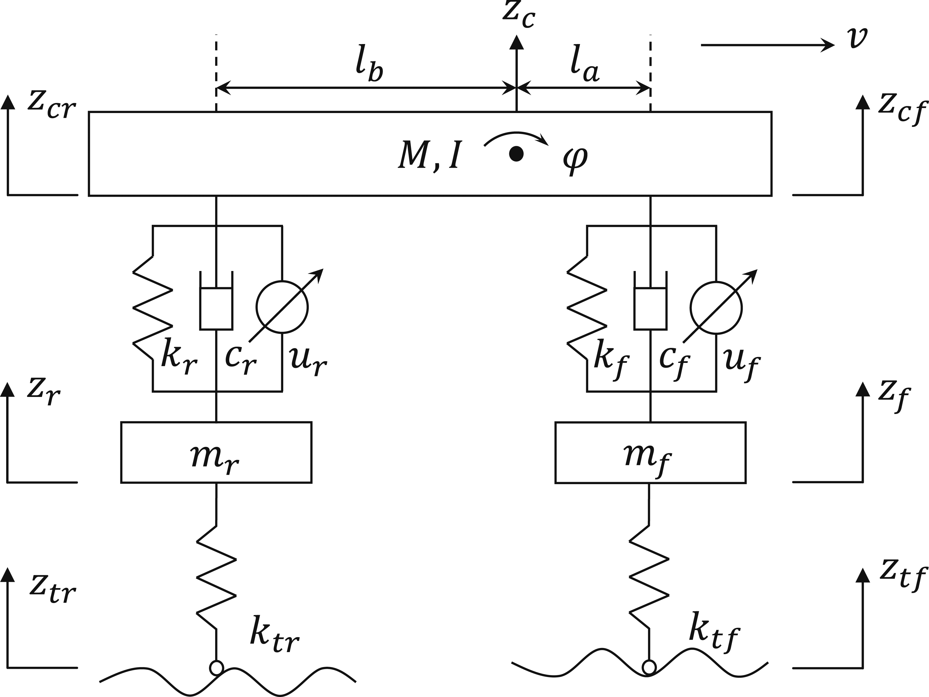
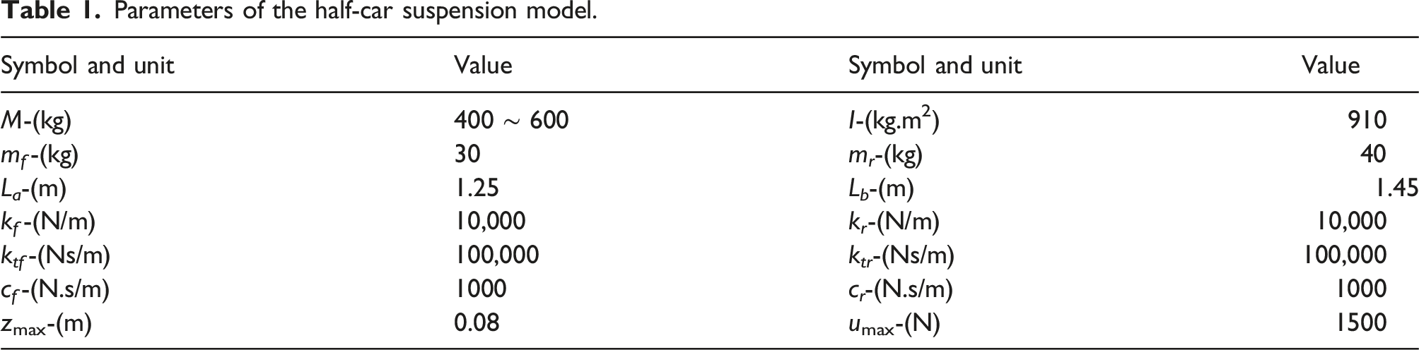
In the figure, M, m, and m r represent the sprung mass of the vehicle and the unsprung masses of the front and rear axles, respectively. I denotes the pitch moment of inertia of the sprung mass. u f and u r represent the control force inputs of the active suspensions at the front and rear, respectively. Furthermore, z f and z r represent the vertical displacements of the unsprung masses. z tf and z tr represent the road surface displacement inputs corresponding to the front and rear wheels of the vehicle, respectively.
Let the vertical displacement of the sprung mass center of gravity be defined as z
c
. Assuming that the pitch angle φ is sufficiently small, it holds that sin φ ≈ φ. Consequently, the suspension displacements at points z
cf
and z
cr
can be simplified as follows:
According to Newton’s second law, the dynamic equations of the suspension system are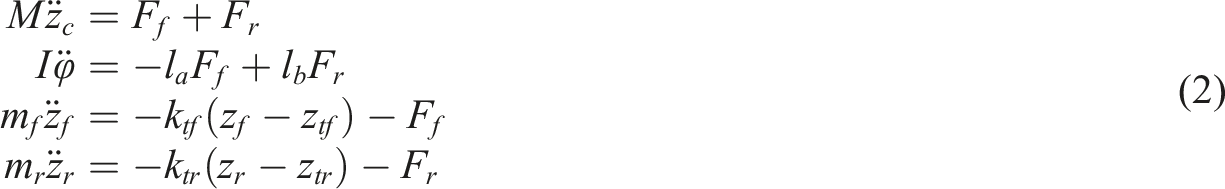

The parameters for the state vector x of the half-car state space equation are as follows
The road input w and the control input force u of the active suspension are described in the following way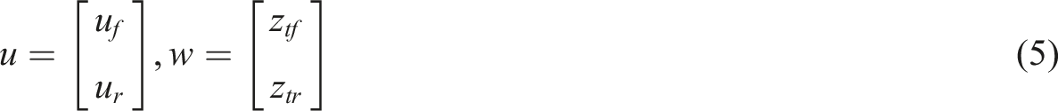
In this article, the suspension model faces the following time domain constraints: 1. The suspension system is located between the body and the wheels and its mechanical components are limited by the vehicle structure. In order to prevent damage from overhandling, it is essential that the controller is designed with the suspension deflection limit in mind 2. There should be a limit to the amount of force that can be applied to the actuator, as the force provided by the active suspension actuator will eventually saturate


The objective of the design of the active suspension controller is to reduce the amount of body vibration, measured in terms of the acceleration of the sprung mass 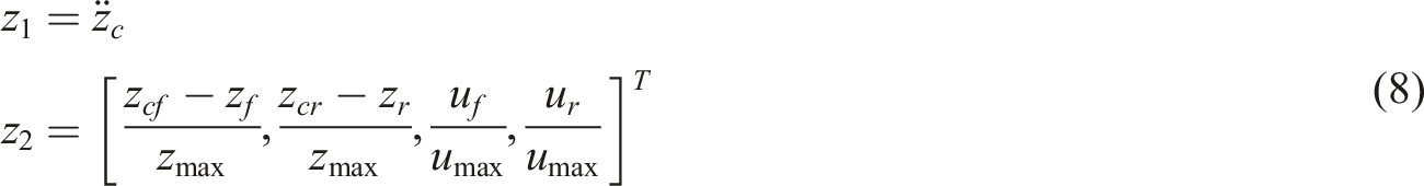
Then we can write the following as the equation of the half car model in its state space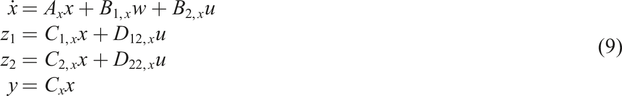
If we assume that the road input z
tf
, z
tr
of the front and rear wheels represent the response of a first order linear filter to a white noise excitation input, as suggested by Prabakar et al.,
29
we obtain the following
Defining the state vector as χ = [x,w]
T
, (9) can be represented in state space as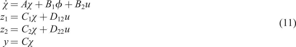
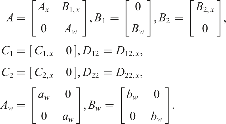
There is a correlation between the matrices A, B1 and the forward vehicle velocity v in (11). To ensure that there is only an affine relationship between the uncertain parameter θ and the system matrices A(θ), B1(θ), we denote the time-varying uncertain parameter as 
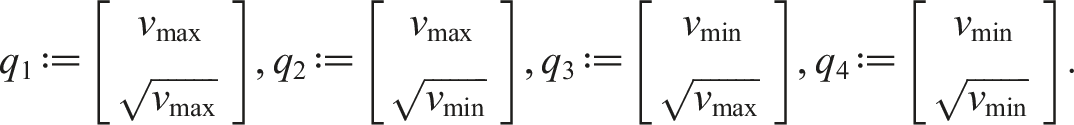
The system matrix associated with uncertain parameters can also be derived from a collection of polyhedral matrices, that is
It may also be shown that the positive scalar α
i
is related to the online observable velocity v by
Changes in vehicle velocity over time are just one of several real world factors that can affect model parameters. The sprung mass of the semitrailer model is also a matter of some debate. For the same reason, we cannot learn anything about how a sprung mass actually works outside of its nominal operating range. By taking the minimum Mmin and maximum Mmax values of the sprung masses M, 1/M can be written as
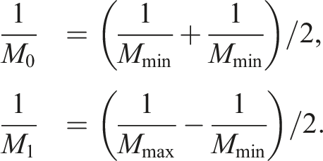
In (11), the state-space matrix with uncertain sprung mass can be rewritten as follows
Main methods
Direct sensing of suspension velocity is difficult in a real vehicle system. The aim of this research is to develop an output feedback H
∞
controller that dynamically modifies the control gain according to the real-time observed velocity v to improve the control performance.

By measuring the current vehicle velocity and calculating the controller’s parameter matrix Ω(θ) in real time, the control gain can be adapted to the changing vehicle velocity. Unlike conventional robust control strategies, which always consider worst-case solutions,31–33 this approach considers all feasible outcomes.
By applying the controller (17) to the system (11), we obtain the closed-loop system defined by 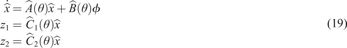
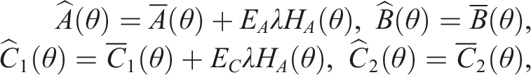
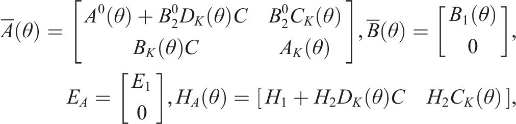


Making the H-value of the closed-loop transfer function matrix G (jω) less than a certain constant γ while maintaining the asymptotic stability of the control system (19) is a common definition of the H
∞
control problem when the finite frequency constraint is taken into account.
In addition, the controlled output z2 must satisfy the following conditions in order to satisfy the time domain constraints of the active suspension (6) and (7)
Before introducing the idea of a finite-frequency robust H ∞ controller that takes into account the uncertainty of the sprung mass, we first offer the following lemmas and theorems.
34
Given positive scalars γ, η, and ρ, the closed-loop system represented by equation (19) is asymptotically stable, and the necessary and sufficient condition for where [F]
s
stands for F + F
T
, and ω
c
= (ω1 + ω2)/2.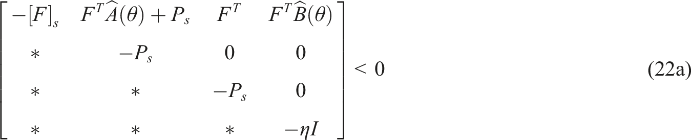
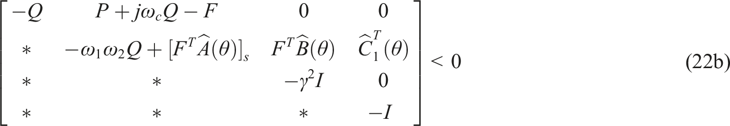

In Lemma 1, inequality (22a) represents the necessary and sufficient condition for the asymptotic stability of the system, (22b) denotes the frequency domain range established according to the KYP lemma, where ω1 ≤ ω ≤ ω2 satisfies the system’s H ∞ performance γ corresponding inequality, and (22c) indicates the necessary and sufficient condition for the system’s time-domain constraint inequality (21). The specific process of inequality proof can be referred to in the literature. 18
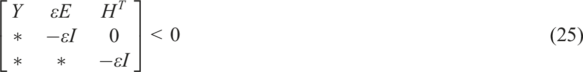
19,34 Given matrices Y, E, and H of appropriate dimension, where Y is symmetric, then If we apply the Schur’s complement to the inequality (24), we get

The asymptotic stability of the system (19) and the necessary and sufficient conditions for
where
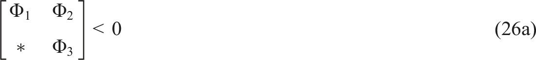
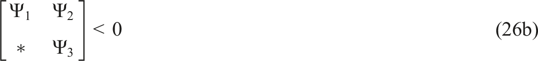

with
and
According to the formulation of Lemma 2, the previous formula is clearly equivalent to the right side of the inequality (26a). Similarly, we can show that (26b) and (26c) correspond to (22b) and (22c), respectively. The proof is completed.
In (26a), (26b), and (26c) the values of
First, the matrix F and its inverse matrix are typically partitioned as follows
If we define
Replace the bilinear term in (26a), (26b) and (26c) with a single linear variable that can be rapidly solved in the following derivation. To facilitate comprehension, we now present the following portion of the variable substitution formula: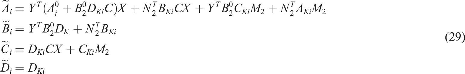
The following H ∞ control theorem for finite frequency robust output feedback can be derived by taking into account the uncertainty of the sprung mass and the influence of the time-varying vehicle velocity.
For given positive scalars γ, η and ρ, the necessary and sufficient condition for the closed-loop system (19) to be asymptotically stable and
where
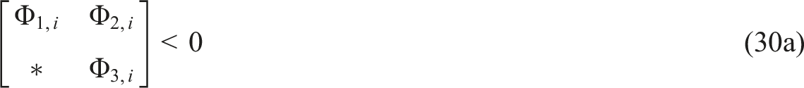
Finally, inequality (30a) is obtained by multiplying the left side of (26a) by J1 and the right side by
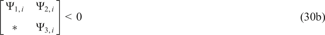
Notice that the matrix to the left of the inequality (30b) has a term for the complex variable jω
c
. According to the method in reference [
35
], a matrix inequality with complex variables can be converted to a higher dimensional inequality as shown below, that is,
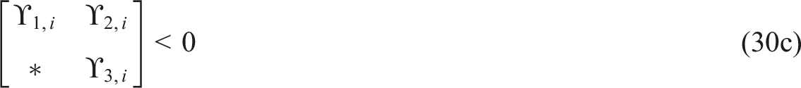
Singular value decomposition always yields the invertible matrices M2 and N2 satisfying (30a), (30b), and (30c) since 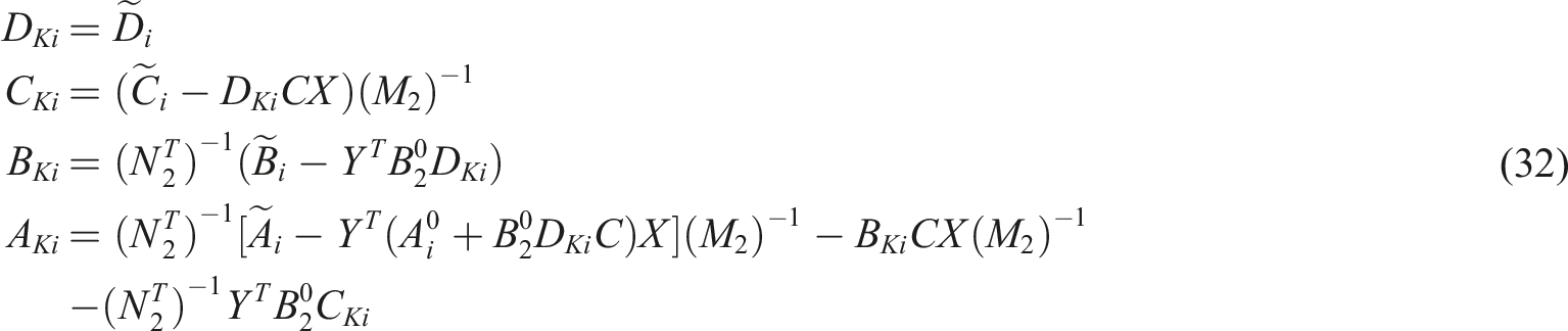
A Ki , B Ki , C Ki , and D Ki can be pre-calculated off-line by combining the above expressions with the polyhedron vertex matrices A i and B1i in (13). The obtained current vehicle velocity v and (18) are used to calculate the velocity related controller matrices A K , B K , C K , and D K in the online stage.
Experiments and results
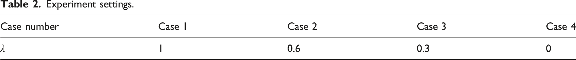
Experiment settings.
Frequency response
Here, we utilize MATLAB and the YALMIP toolbox to solve the positive definite programming problem (30a), (30b) and (30c). The control gain matrices A Ki , B Ki , C Ki , D Ki , i = 1, …, 4 are computed by setting the finite frequency constraint parameters to the values specified in Sun et al (2010). 18 Specifically, we select w1 = 4, w2 = 8, η = 10,165 and ρ = 0.9. The control methods used for comparison in this section include:
1. Passive: where the control force is neglected, assuming a constant value of zero;
2. Entire: a dynamic output feedback H ∞ controller solved over the entire frequency range, as referenced in Sun et al.(2011) 36 ;
3. Proposed: the robust finite frequency H ∞ controller described in this study, which depends on vehicle velocity.
The comparison of different control methods aims to validate the effectiveness of the proposed approach in ensuring vibration control within the human sensitivity frequency range of 4–8 Hz, under time-varying parameters.
Figure 2 displays the frequency response of the sprung mass acceleration Frequency responses of sprung mass acceleration. Passive (- -), Entire frequency (- · -), Finite frequency —. (a) v = 10 m/s, (b) v = 20 m/s, (c) v = 30 m/s, (d) v = 40 m/s.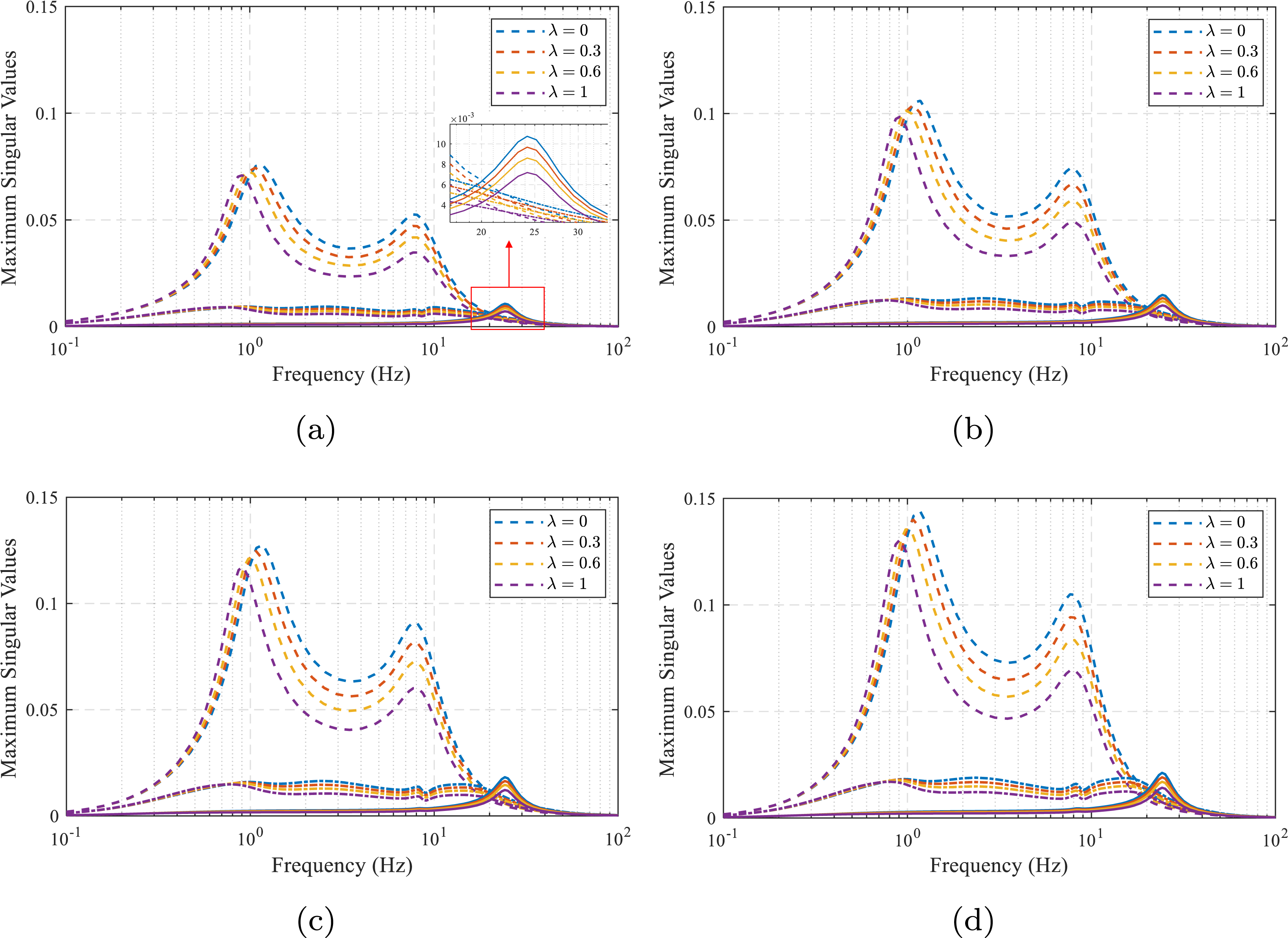
Figure 3 presents a comparison of the H
∞
performance for passive control, entire frequency control, and the finite frequency controller calculated based on Theorem 2 under varying sprung mass and velocity conditions. In the figure, the sprung mass varies along the X-axis, velocity along the Y-axis, and the H
∞
performance value of the closed-loop system is displayed along the Z-axis to evaluate the impact of different parameters on the disturbance performance of the suspension system. The results indicate that under passive control conditions, the system’s H
∞
performance is relatively insensitive to changes in sprung mass, whereas velocity has a significantly greater effect on H
∞
performance than sprung mass. In contrast, both entire frequency control and finite frequency control strategies markedly improve the H
∞
performance metrics of the closed-loop system, demonstrating enhanced disturbance rejection capabilities. Notably, at higher velocity, the finite frequency control method achieves superior H
∞
performance compared to the entire frequency controller. Effect of sprung mass and velocity on H
∞
control performance. (a) Passive, (b) Entire frequency, and (c) Finite frequency.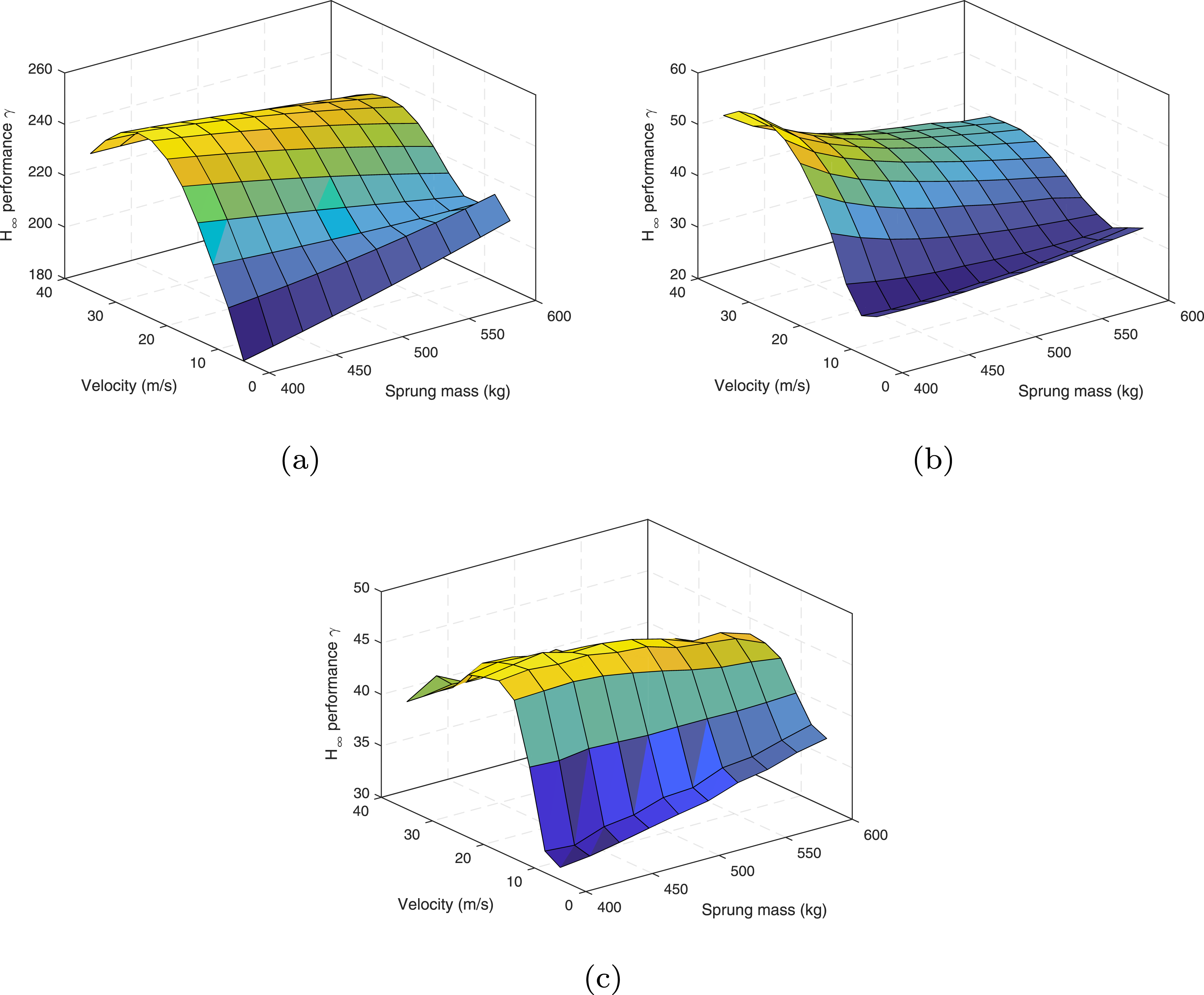
Time response
The efficiency of the proposed controller in time-varying vehicle velocity scenarios is further evaluated by performing time-domain simulations for the two vehicle velocity variation circumstances shown in Figure 4, Scenario I and Scenario II, respectively. Two different scenarios of velocity changes. (a) Scenario I, (b) Scenario II.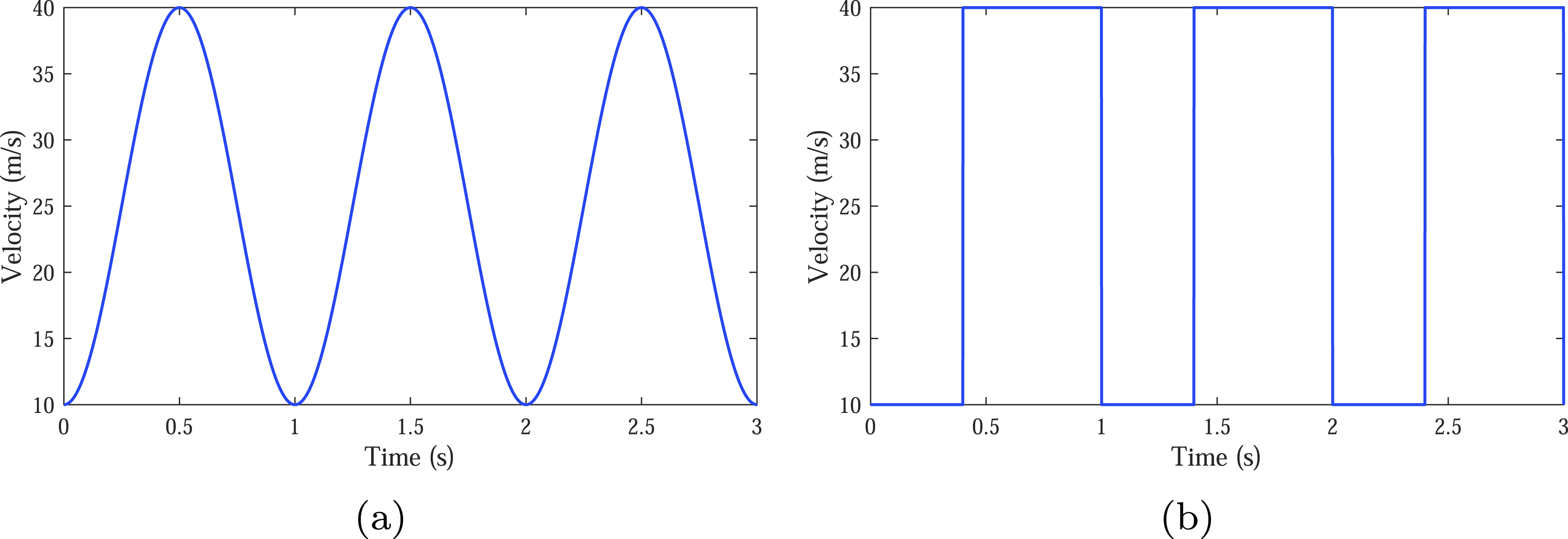
First, we compare the proposed velocity-dependent finite frequency control method (LPV) with traditional linear time-invariant (LTI) finite frequency controllers by adding an additional constraint A
Ki
= A
K
, B
Ki
= B
K
, C
Ki
= C
K
, D
Ki
= D
K
, i = 1, …, 4 in inequality (30). The comparison includes LTI controllers operating at constant velocities of 10 m/s (LTI-10) and 40 m/s (LTI-40). Figures 5–8 present the root-mean-square (RMS) values of the sprung mass acceleration under ISO-B, ISO-C, ISO-D, and ISO-E road conditions. It should be noted that these simulations consider the sprung mass under the conditions specified in Case 1, without accounting for the uncertainty of sprung mass in other cases. The comparison is solely between the traditional constant-velocity finite-frequency H
∞
control method and the velocity-dependent robust finite-frequency H
∞
control method proposed in this study. Time-domain body acceleration responses on ISO-B road. (a) Scenario I, (b) Scenario II. Time-domain body acceleration responses on ISO-C road. (a) Scenario I, (b) Scenario II. Time-domain body acceleration responses on ISO-D road. (a) Scenario I, (b) Scenario II. Time-domain body acceleration responses on ISO-E road. (a) Scenario I, (b) Scenario II.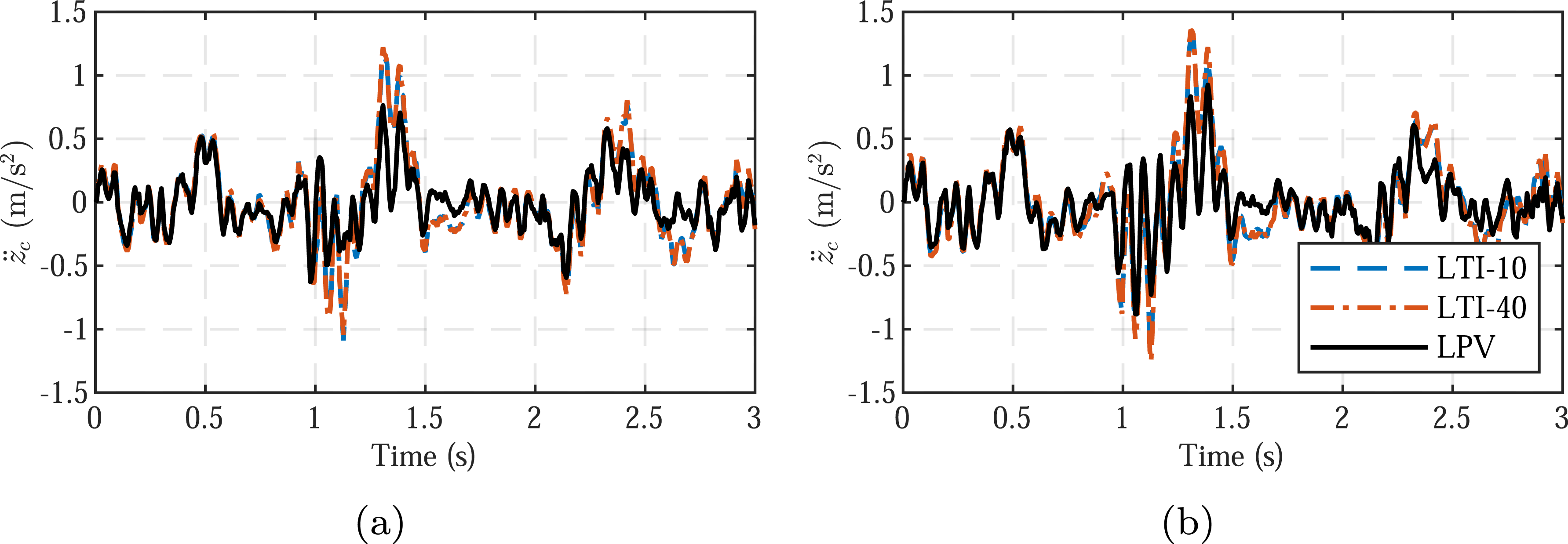
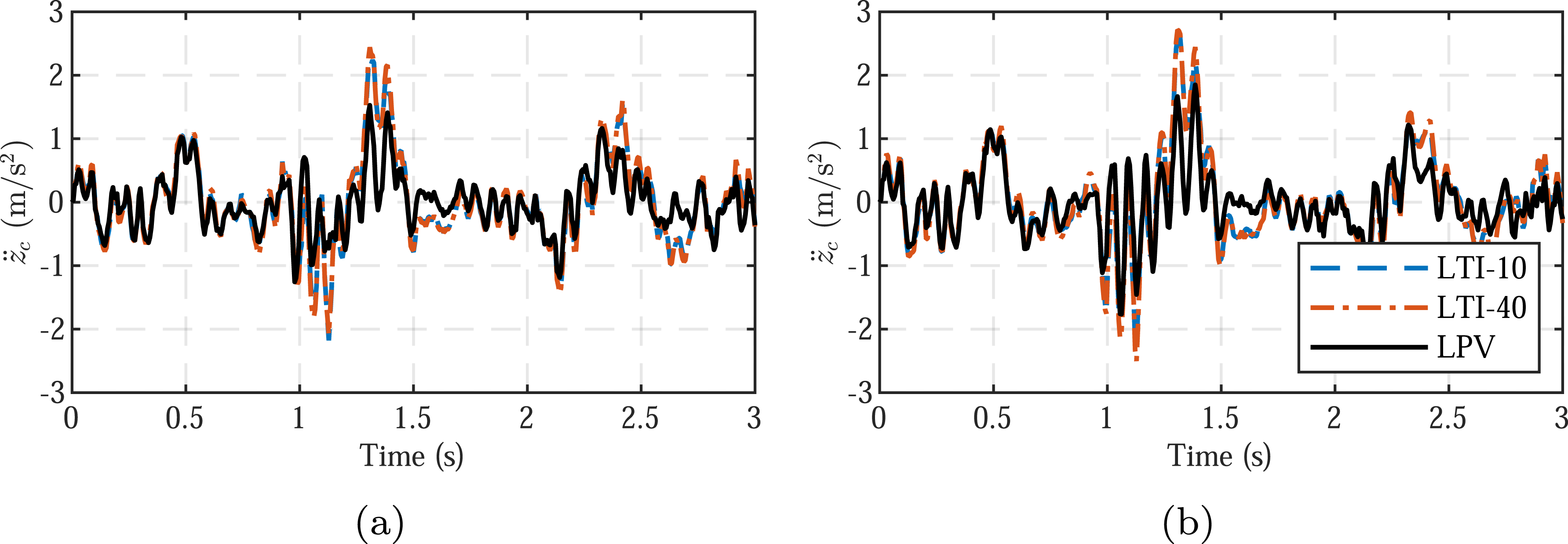
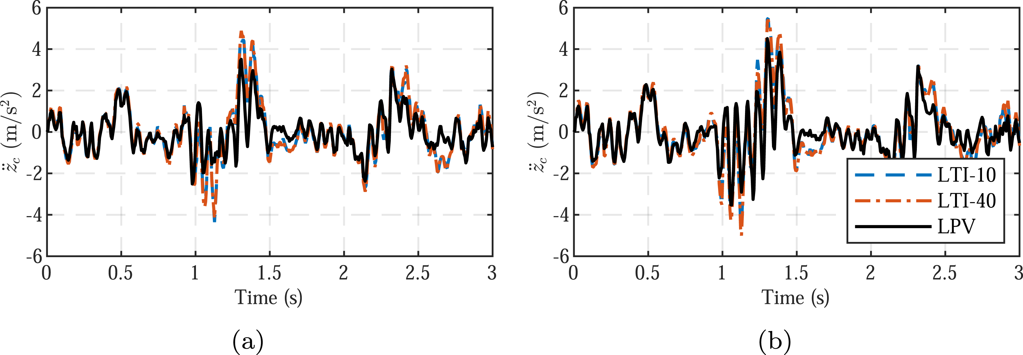
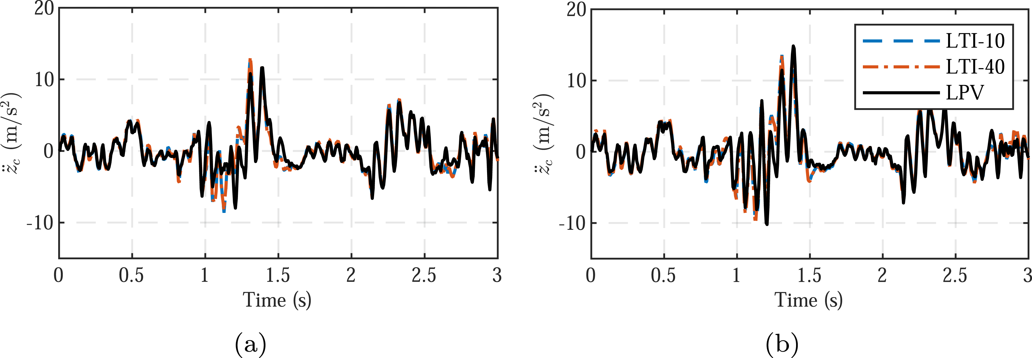
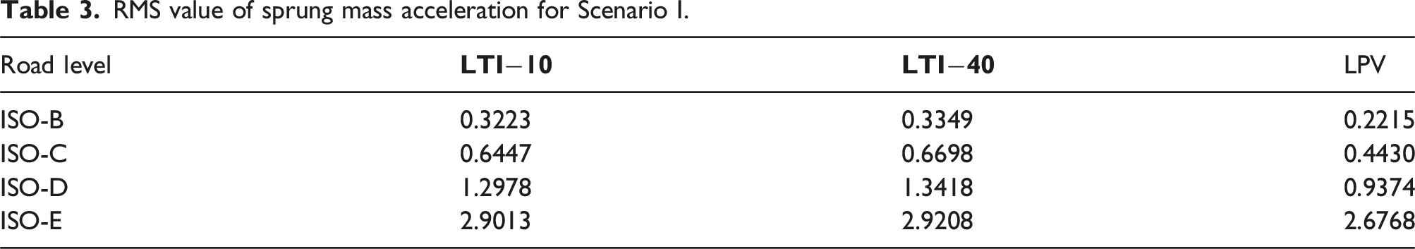
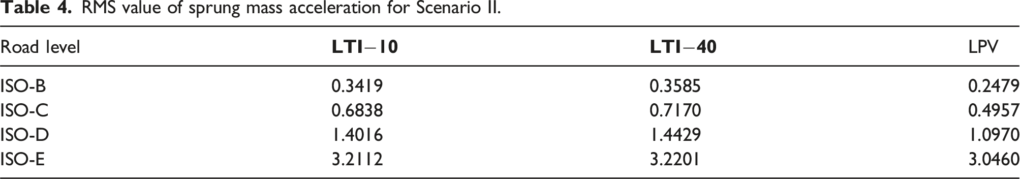
The results indicate that as the road quality increases, the RMS peak values of acceleration also exhibit an increasing trend. Notably, under ISO-E road conditions, the performance difference between the constant velocity and velocity-dependent control methods becomes negligible. This is attributed to the saturation of control inputs under high road inputs, where the effectiveness of either control method in reducing sprung mass acceleration is limited. In contrast, under lower road input conditions observed in ISO-B, ISO-C, and ISO-D, it is evident that the velocity-dependent finite frequency H ∞ control method effectively reduces the RMS values of sprung mass acceleration compared to the constant velocity control method.
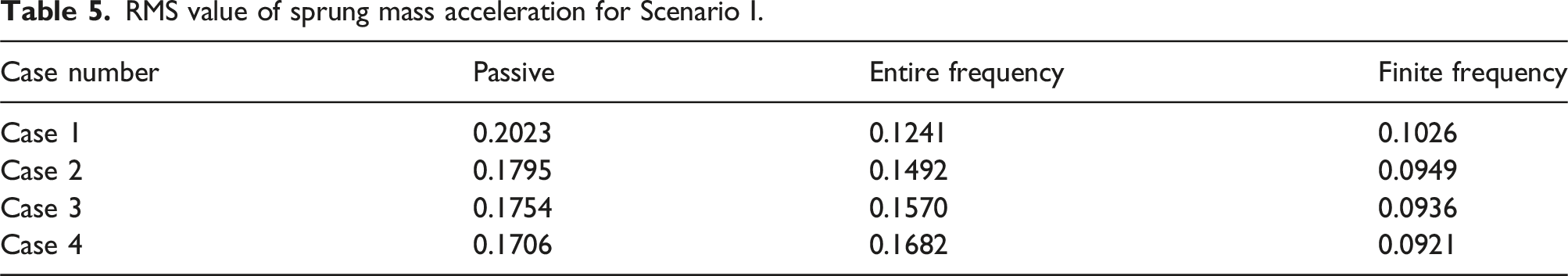
RMS value of sprung mass acceleration for Scenario I.
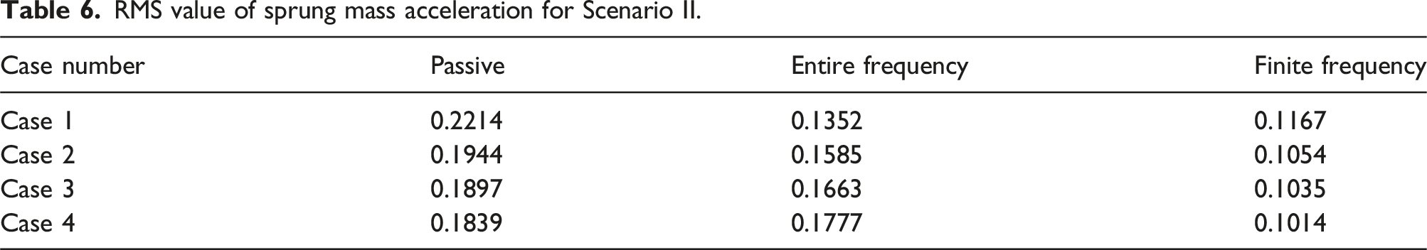
RMS value of sprung mass acceleration for Scenario II.
Furthermore, we evaluate the vibration control performance of the suspension system under ISO-A random road conditions. The reference spatial frequency for the ISO-A road is given by G
q
(n0) = 16 × 10−6 m3. Figures 9 and 10 illustrate the time-domain response of the vertical acceleration of the sprung mass Time-domain body acceleration responses for Scenario I. (a) Case 1, (b) Case 2, (c) Case 3, (d) Case 4. Time-domain body acceleration responses for Scenario II. (a) Case 1, (b) Case 2, (c) Case 3, (d) Case 4.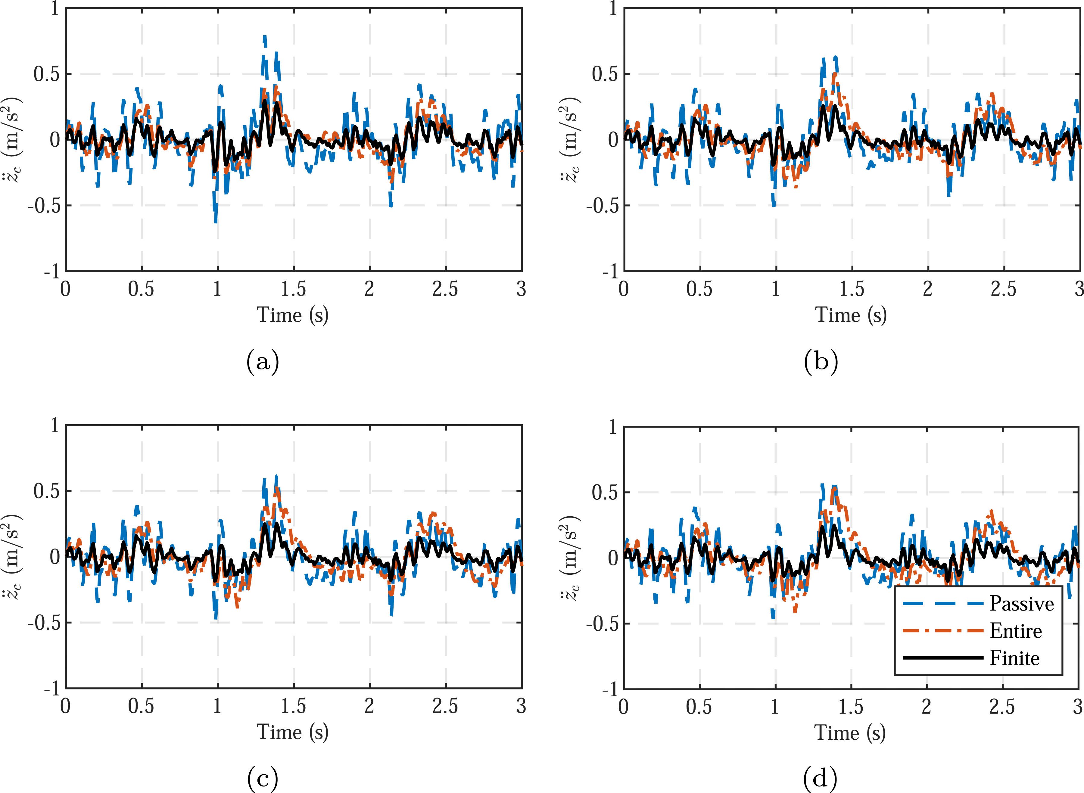
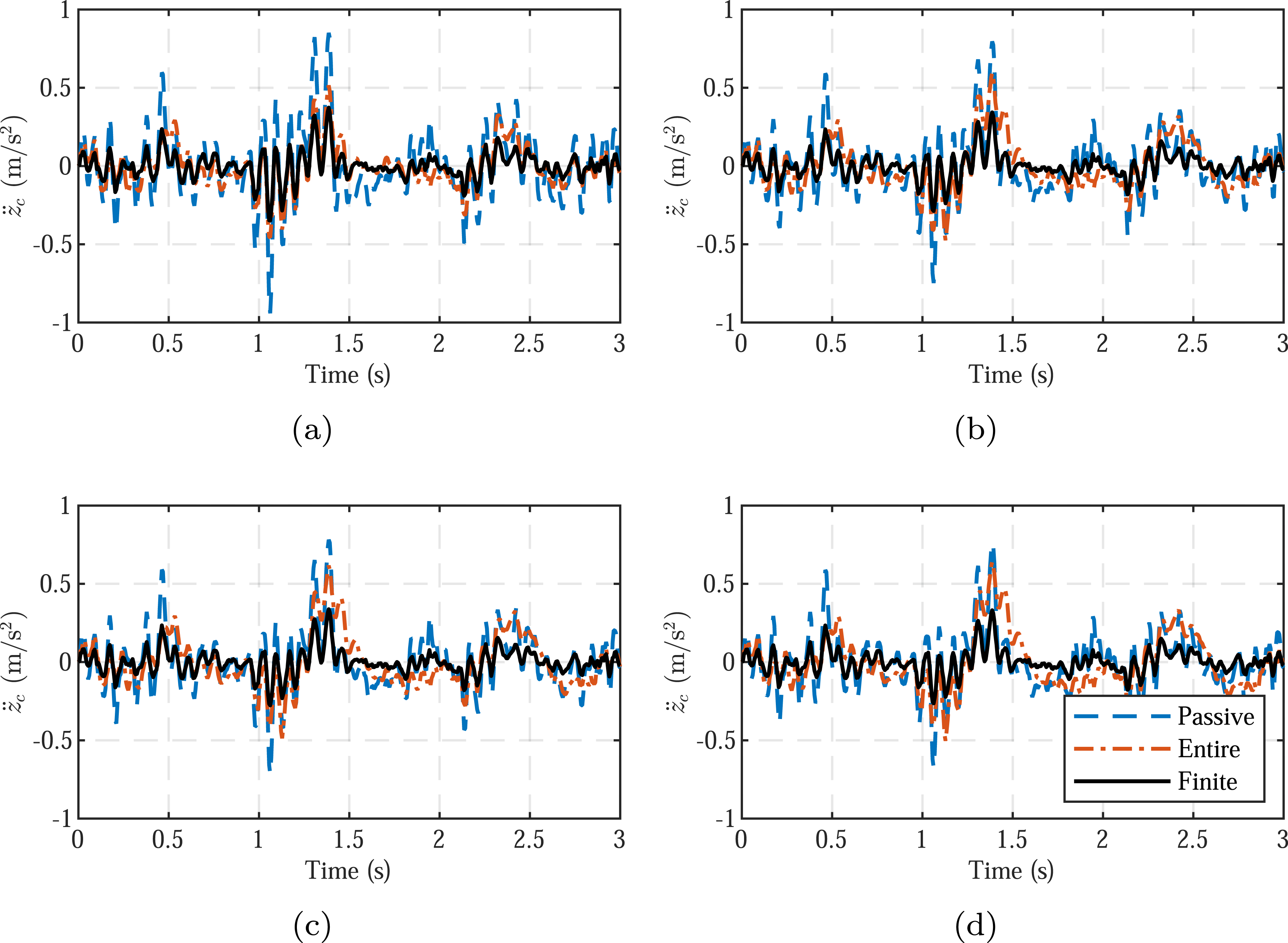
Figure 11 illustrates the variation in suspension dynamic stroke and actuator control force under changing vehicle velocities in Scenario I, with similar trends observed in Scenario II. The results indicate that, under ISO-A road conditions, both the suspension dynamic stroke and actuator control force remain below the maximum limit, specifically z2 < 1. Therefore, inequality (30c) effectively ensures the desired time-domain constraints are met. Suspension deflection and control force under Scenario I. (a) front suspension deflection, (b) rear suspension deflection, (c) front control force, and (d) rear control force.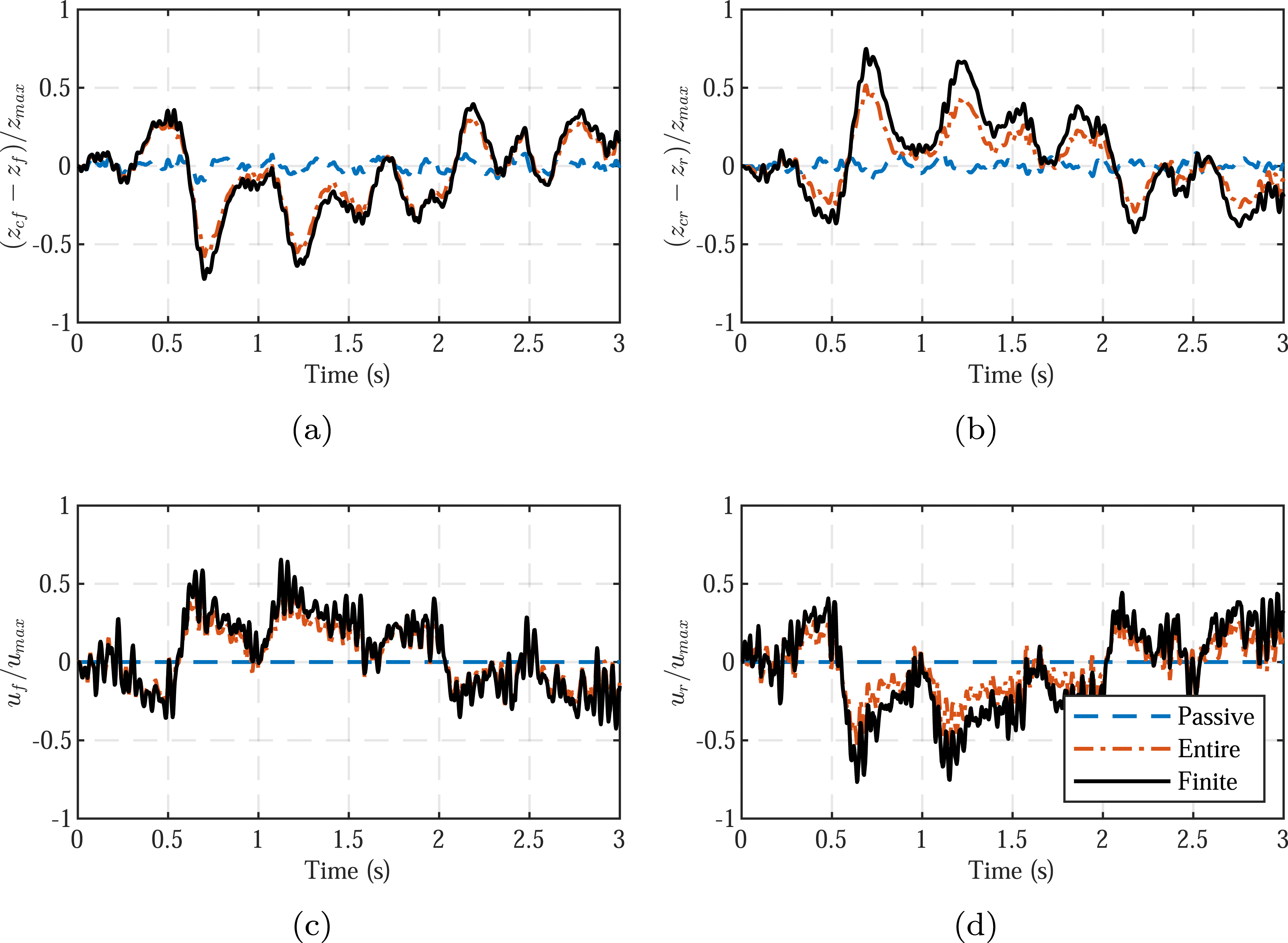
RMS value of sprung mass acceleration for Scenario I.
RMS value of sprung mass acceleration for Scenario II.
Conclusion
This study has developed a velocity-dependent robust finite frequency H ∞ control strategy for a half-car model, capable of meeting the vibration suppression objectives of active suspensions under various sprung mass conditions. Compared to traditional finite frequency H ∞ control methods with constant parameters, the proposed control strategy significantly reduces the root-mean-square (RMS) value of vertical acceleration by approximately 21% to 31% under varying velocity conditions. It also satisfies the predefined time-domain constraints on suspension displacement and control force. This addresses the decline in vibration suppression performance in the human sensitivity frequency range under uncertain sprung mass and vehicle velocity conditions. However, there are still some limitations in this study, as it focuses solely on the vertical acceleration of the sprung mass as the control objective and does not consider the optimization of pitch angular acceleration. In the future, we will consider multi-objective optimization methods to achieve a balance and compromise among multiple control objectives.
Footnotes
Declaration of conflicting interests
The author(s) declared no potential conflicts of interest with respect to the research, authorship, and/or publication of this article.
Funding
The author(s) disclosed receipt of the following financial support for the research, authorship, and/or publication of this article: This work was supported by the National Key Technologies Research and Development Program of China (2018YFB0106200).