
Abstract
To address the challenge associated with optimizing the number and positioning of accelerometer points in ship acoustic reconstruction, factor analysis is applied to the automatic optimization of accelerometer position in this work according to the source independence of ship’s underwater radiated noise. Based on the numerical simulation method that calculates the vibration noise response under specific operation conditions, the minimum number and the optimal position of the accelerometers can be obtained through the factor analysis and multi-parameter comprehensive evaluation method. The results of acoustic reconfiguration and testing are compared using one test cabin as a validation object to verify the effectiveness of the proposed method. The results show that the automatic optimization algorithm can improve the reconstruction accuracy concerning the uniform distribution method. The error is reduced from 15.46% (1.5 dB) to 8.35% (0.8 dB), and the correlation coefficient is improved from 0.86 to 0.89. The semi-automatic optimization method is slightly lower in terms of errors and correlation coefficients compared to the automatic optimization algorithm. After increasing the number of monitoring positions for automatic optimization, the acoustic reconstruction accuracy is further improved, while the average error is reduced to 7.37% (0.7 dB) and the correlation coefficient is improved from 0.89 to 0.92. The experimental results are proximate to the conclusions of the simulation calculation. Even under the circumstance of multi-factor noise interference, the correlation coefficient of multi-position automatic optimization can still reach 0.8, in comparison with the uniform distribution method, the error is reduced from 32.49% (3.4 dB) to 25.94% (2.6 dB). The proposed method effectively captures the dynamic characteristics of complex structures and their impact on underwater radiated noise, and the integration of factor analysis can prominently enhance the computational efficiency, thereby providing technical support for engineering applications to the ship acoustic reconstruction.
Keywords
Introduction
As a complex aquatic structure, hulls are subjected to various exciting forces during the operation of internal equipment, resulting in vibration and noise.1–3 Underwater radiated noise from ships constitutes a significant portion of the low-frequency marine ambient noise. As the continuous development of the shipping industry, the noise level in the marine environment is continuously increasing.4–6 The higher underwater noise environment not only adversely affects the sensory systems and ecology of marine life7–9 but also affects the detection accuracy and efficiency of ships equipped with precision acoustic instruments. Therefore, ship classification societies in various countries have proposed guidelines for the control and testing of underwater radiated noise.10–12 Over the past few decades, numerous methodologies have been developed to measure the underwater radiated noise generated by ship structures, 13 including the finite element or boundary element method for low-frequency noise,14–16 and the statistical energy analysis method for high-frequency noise. 17 Among them, the acoustic boundary element method has been widely used in the calculation of ship radiation noise and has shown high accuracy and effectiveness. 18 Underwater radiated noise is mainly caused by propeller noise and mechanical noise of the hull structure. Propeller noise can be directly measured by the hole drilling method at the stern of the ship, while the mechanical noise of the hull cannot be directly obtained since the hull structure is a complex structure of several hundred meters in length. Therefore, accurately measuring or predicting the vibration distribution on the surface of the hull structure is crucial for predicting underwater radiated noise. 19
Vibration and noise monitoring and analysis are key technologies for assessing the operating conditions of mechanical equipment and its impact on the environment.20–27 Vibration measurement engineering for large structures faces many challenges. Traditional methods require the manual deployment of hundreds of accelerometer s and a large amount of signal cables, which is not only labor-intensive but may also affect the dynamic characteristics of the structure. 28
Additionally, the deployment of accelerometers that are not reasonably placed or are insufficient in number can affect the accuracy of the measurement results. Therefore, the optimized arrangement of accelerometers in the vibration measurement of large structures is particularly necessary. The optimized arrangement of accelerometers not only allows the complete vibration response field of the structure to be reconstructed through limited measurement data but also provides sufficient spatial resolution while avoiding the cost and complexity associated with dense measurement. 29 This strategy not only improves data quality but also reduces interference with the natural vibration behavior of the structure, providing reliable data support for structural health monitoring and analysis.
From an engineering perspective, people generally prefer to use vibration sensors on the hull surface as few as possible while the accuracy for prediction can still be maintained. Due to military and commercial reasons, open literature is scarce on the issue of sensor placement in underwater radiated noise monitoring systems. In the investigation of equipment load inversion and the monitoring of underwater radiated noise, it has been found that the recognition accuracy of many algorithms largely depends on the placement of measurement positions (including the number and position of the points). Wang et al. 30 introduced two distinct sensor placement strategies grounded in the conditional analysis of the Markov parameter matrix, they defined the sensor-related transfer function matrix and incorporated ill-conditioning criteria related to the Markov parameter matrix into their methodology. In response to the limited problem of sensor location and quantity in the modal testing process of asymmetric large-span bridge structures, Satpathi et al. 31 proposed the kinetic energy optimization technique (EOT) and compared it with the effective independence method (ElM) algorithm proposed by Kammer. 32 The main advantage of this method is the optimization of the number of sensors. He et al. 33 used the establishment of a cylindrical shell acoustic model to compare the far-field acoustic pressure, and they proved the feasibility of the uniform sensor placement method adopted by the American and French navies through theoretical analysis and numerical simulation. The real-time visualization of underwater radiated noise cannot be separated from the vibration and noise monitoring signals. Yin 34 conducted node clustering based on the finite element calculation modal results. They initially selected the measuring positions using the effective independence method and then multiple evaluation parameters were adopted comprehensively as the criterion for position selection. They also used the genetic algorithm for optimization and determined the layout position of the vibration sensor. Wang 35 based on the ill-posed problem in the dynamic load identification process and proposed a correlation analysis method based on the minimum ill-posed criterion based on the Markov parameter matrix, which can quickly obtain the location of accelerometer with great stability and high calculation accuracy.
In the realm of structural health monitoring, substantial advancements have been made in optimizing sensor position. Researchers have proposed a variety of detection methods, including vibration monitoring, strain monitoring, and monitoring based on elastic waves, 36 and they have developed a variety of sensor placement optimization techniques, such as the Effective Independence Method, 37 the Minimum Modal Assurance Criterion, 38 and the Modal Matrix Summation and Integration Method.39,40 The classic methods, such as the Effective Independence Method and the Modal Kinetic Energy Method, typically use sequential or reverse selection strategies. They start from all measurement positions and gradually identify and eliminate the degrees of freedom that have the least impact on structural performance.41–43 However, as stated in the literature, 44 these methods are significantly effective when dealing with small-scale structures with fewer degrees of freedom, but their efficiency drops sharply when facing structures with numerous degrees of freedom. Thus, the problem of an optimal sensor layout is essentially a complex discrete combinatorial optimization problem, and traditional optimization techniques are difficult to be applied due to the lack of gradient information.
As large-scale models, ships have complex internal structures with tens of thousands of potential nodes, which make classical algorithms clearly inefficient. Therefore, this paper introduces factor analysis theory that is a data dimensionality reduction model. Its basic idea is grouping variables according to the degree of correlation. Variables within the same group exhibit high inter-correlation, whereas variables across different groups remain uncorrelated. Each group of variables represents a fundamental structure identified as a common factor. 45 The groups obtained after rotating the factor loading matrix have more practical physical significance. Few scholars have considered the impact of monitoring positions on both vibration response and underwater radiated noise and determined the optimal monitoring positions through comprehensive indicators, such as vibration independence and the relationship between vibration and acoustics.
In summary, a method that combines factor analysis has been proposed for dimensionality reduction with a multi-parametric comprehensive evaluation that considers both vibration independence and the correlation between vibration and acoustics, meanwhile the corresponding contribution factors can be adjusted by parameters. This approach can significantly enhance the efficiency of solving problems and provide a new technical approach for ships vibro-acoustic reconstruction, which has important theoretical significance and practical value.
The primary objective of this work is to optimize the placement of accelerometers for ship acoustic reconstruction by employing factor analysis, thereby enhancing the accuracy and efficiency of vibration monitoring. This study seeks to establish a systematic framework for selecting optimal measurement positions that can be adapted to various applications within the field of low-frequency noise and vibration analysis.
Framework of research methods
Overall framework of accelerometer automatic optimization
This research presents a groundbreaking application of factor analysis aimed at optimizing accelerometer placements in ship acoustic reconstruction, a technique that significantly improves measurement efficiency and accuracy. In contrast to traditional methods that depend on uniform distribution, our approach employs multivariate statistical analysis to identify and select accelerometers based on independent vibration sources. This innovative integration of statistical methodologies into acoustic monitoring marks a substantial advancement in the field, with the potential for broader applications in noise and vibration analysis across various engineering domains.
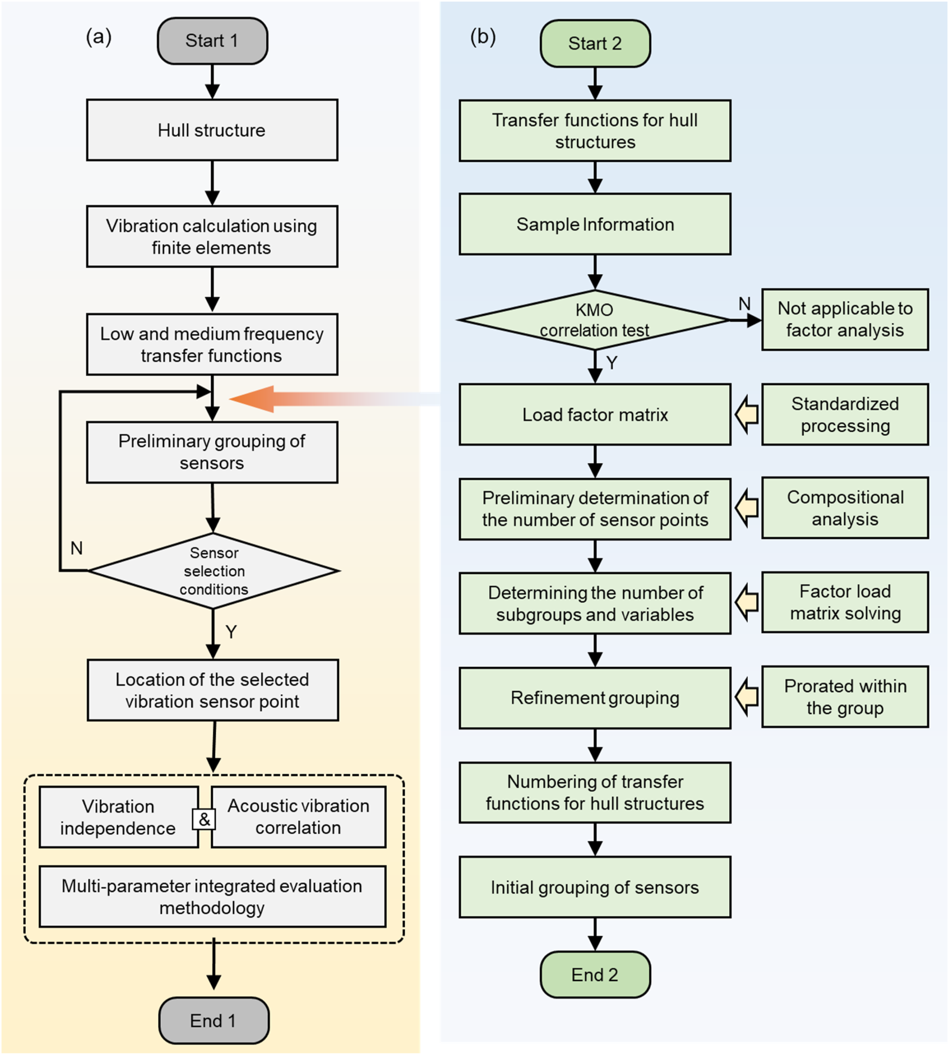
The automatic optimization process for measurement positions relies on the hull structure transfer function. The main idea of the joint automatic optimization method based on the factor molecule method and the multi-parametric comprehensive evaluation method is shown in Figure 1: (1) A finite element model is constructed based on the hull structure diagrams; (2) Excitations are applied at the positions of the main power equipment to capture the structural vibration response of the entire ship. Subsequently the vibration transfer function within the medium and low-frequency ranges is analyzed; (3) Utilizing the factor analysis method, all nodes of the entire ship are grouped into several sub-areas (detailed steps of factor analysis will be described later); (4) Determine whether the preliminary grouping is appropriate to ensure that at least one accelerometer measurement locates in the concerned sub-areas; (5) After data dimensionality reduction, evaluate the vibration independence of each candidate monitoring position within each group, and simultaneously evaluate the sound-vibration correlation of each candidate monitoring position within each group; (6) According to the research focus, check the evaluation of vibration independence and sound-vibration correlation, which determines the final accelerometer position through the multi-parametric comprehensive evaluation method. (a) Flowchart for the selection of vibration monitoring positions based on factor analysis method; (b) Concept of selecting vibration accelerometer monitoring positions based on factor analysis method.
Framework of factor analysis
The detailed steps of the factor analysis method are outlined in Figure 1(a) and the processes of selecting vibration accelerometer monitoring positions are shown in Figure 1(b): (1) Obtain the low-frequency vibration transfer function of the hull structure under a certain working condition as sample information; (2) Use the KMO (Kaiser–Meyer–Olkin) test to determine whether a set of variables is suitable for factor analysis. The KMO test evaluates the adequacy of the correlation matrix for factor analysis by comparing the simple correlation coefficients with the partial correlation coefficients between variables. Generally, the KMO value greater than 0.6 is suitable for factor analysis, and values closer to 1 are better. If the KMO test is not met, other data analysis methods should be used; (3) Calculate the mean and variance of the sample data, then standardize the data. This process yields the factor loading matrix, which represents the relationships between the standardized sample information and the underlying facto; (4) Solve the eigenvalues and eigenvectors of the factor loading matrix based on the principal component analysis method, sort the eigenvalues from largest to smallest, and preliminarily determine the number of common factors based on the contribution required by the system; (5) Solve the factor loading matrix, rotate the matrix to maximize variance, and divide several groups based on the loading coefficients. Divide variables with larger loading coefficients into one group to determine the total number of groups and the variables within each group; (6) Proportionally allocate the number of accelerometers for each group, ensuring that at least one accelerometer is allocated for each group of variables; (7) Repeat the above steps for each group to further refine the group, or refine the grouping again according to the number of variables in each group and the required number of accelerometers by defining a specified number of factors; (8) Classify all nodes in the transfer function according to the refined grouping, and then the preliminary grouping of accelerometers can finally be obtained.
Relevant theories of automatic optimization methods for measuring positions
Similarity principle and physical significance
The acoustic reconstruction of the hull is essentially a combination of the first and second types of structural dynamic problems. By placing a limited number of vibration accelerometers on the structure, the 3D acoustic field distribution of large-scale hull structures is reconstructed based on the structural transfer function.
In the context of studying structural transfer functions, factor analysis can be used to determine the number of common factors and group variables with strong correlations together. The number of common factors corresponds to the number of independent excitation sources. The load matrix corresponds to the transfer function, while the specific factors correspond to the error terms, which can be ignored in practical analysis.
Under the action of steady-state loads, the structural dynamics equation is given by
46

The factor analysis model is
47

Comparing the two formulas mentioned above without considering the specific factors, it is not difficult to find that the load matrix
Transfer function solution method
The vibration system composed of the base and the hull will inevitably cause a response in other parts when subjected to an external excitation. The damped forced vibration dynamics differential equation is given by
48

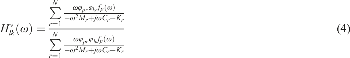
Under the action of a single-point excitation, the correspondence between the external load and the response of the structure is determined by the system’s transfer characteristics, that is, the transfer function. The vibration velocity at both the structural vibration monitoring points and the acoustic reconstruction locations is determined using the modal superposition method.
The transfer function from position l to position k is
48
The method of accelerometer position selection based on factor analysis method
If the finite element model of the hull structure has
The problem is how many monitoring positions are needed at least to achieve the reconstruction of the vibration and noise throughout the ship, and how the monitoring accelerometers should be arranged. To solve this problem, the factor analysis method needs introducing. Suppose there are p original variables


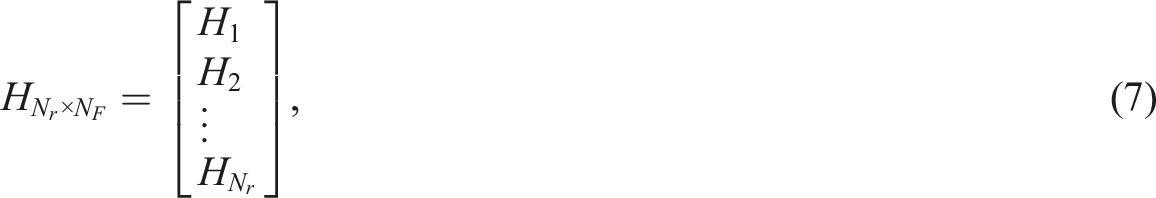
The matrix
There are many methods to solve the factor loading matrix, mainly the following three ones: principal component analysis, principal factor method, and maximum likelihood estimation. Consider that the principal factor method might not capture as much total variance as PCA and maximum likelihood estimation require more assumptions about the data distribution. The principal component analysis method is used in this work, and its principle and the main calculation steps are stated as follows: (i) Calculating the covariance array (ii) Calculating the eigen roots of the covariance array (iii) Using the eigenvector matrix
The obtained factor loading matrix
The rotation of the loading matrix is divided into two types: orthogonal rotation and oblique rotation. Common methods for orthogonal rotation include the Varimax method, the quartimax method, and the equamax method. Common methods for oblique rotation include the minimum oblique rotation method, the quartimin method, oblique rotation, etc. This study adopts the Varimax method of orthogonal rotation for research to obtain preliminary groupings, that is, to divide all nodes in the original structural vibration transfer function into several sub-areas. Nodes within each area have similar structural dynamic characteristics. However, there may be differences in dynamic response between different areas possibly due to the bending and turning of vibration waves during structural transmission, such as T-shaped profiles in hull structures, or the process of transmission from horizontally arranged mechanical decks to bulkheads.
Vibration independence
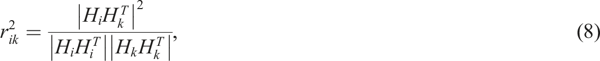
Different locations of response positions will affect the ill-conditioning of the transfer function matrix. The location of a response position determines a row of elements in the matrix. The linear relationship between response positions can be obtained by analyzing the relationships between row vectors. The transfer function matrix at a certain frequency can be rewritten as
51
The row coherence coefficient of the


Vibro-acoustic correlation
The indicators of acoustic correlation are designed to describe the consistency between the vibration information at the monitoring positions and the variation patterns of radiated noise. The better the consistency between them, the more effective the selection of the measurement positions is.
The calculation formula of vibro-acoustic coupling can be derived as
52

To describe the consistency of acoustics and vibration, it is necessary to select parameters for quantitative analysis. The Pearson correlation coefficient, also known as the correlation similarity, is a statistical approach that reflects the degree of similarity between variables. Its value is the covariance between X and Y
49

In addition, the quantity that characterizes the correlation between X and Y is
49

The value range of
In terms of vibro-acoustic correlation, a correlation coefficient is used here to statistically analyze the correlation between ship’s structural vibration and underwater radiated noise. Then, the interrelationship between them can be obtained. The correlation coefficient

Comprehensive evaluation indicators
Considering independence of vibration and the correlation of sound and vibration, a comprehensive approach is proposed to consider various indicators to ensure a rational arrangement of accelerometers. In addition, normalization methods are used to avoid scale issues, and a comprehensive evaluation index is used as the objective function to assess the rationality of the accelerometer layout, which is expressed as
50

After the preliminary groups are obtained, the principle of selecting measurement positions within each group is to maximize the vibration independence of the selected measurement positions’ and to ensure the best correlation between sound and vibration. This approach can not only avoid the issue of matrix singularity during the inversion process but also select measurement positions with high vibro-acoustic correlation.
Models and boundary condition settings
Models of cabin segment
A cabin model is used as a benchmarking object, and its typical sectional schematic is shown in Figures 2(a) and (b). The model simulates the primary excitation source of the ship, which is the cabin segment. This segment is approximated as a cylindrical shell with an internal deck and columns. The outer plate has a thickness of 9 mm, the end panels are 12 mm thick, the main deck is 8 mm thick, and the top deck is 12 mm thick. All steel plates are reinforced with various cross-sectional profiles, and the lower part of the main deck is supported by three columns. The main excitation devices are seawater pumps and exciters, which are connected to the hull through the pedestal, and the shape of the actual cabin segment and the internal test site are shown in Figures 2(e) and (f). (a) Side view and (b) longitudinal sectional view of the cabin segment; (c) overall and (d) longitudinal sectional finite element model of the cabin segment; (e) external physical view of cabin segment; (f) interior acoustic test site of cabin segment.
To calculate the vibration and radiated noise of the cabin segments, the corresponding finite element models are built according to Figures 2(a) and (b), as shown in Figures 2(c) and (d). In the developed finite element model, the internal ballast water is simulated using three-dimensional fluid elements with a bulk modulus of 1.5 × 10⁶ kg/(m2·s). Shells are represented by two-dimensional shell elements, while columns and profiles are modeled with one-dimensional beam elements. The device is treated as a zero-dimensional plasmonic element and is connected to the base via an MPC. All wet elements immersed in water are oriented outward, and the attached rippled water is accounted for using the “MFLUID” command in the NASTRAN card. The complete finite element model of the outer plate consists of approximately 8463 nodes and 16,157 elements.
Based on the developed finite element model, the main calculation process of vibration response can be expressed as follows: (i) conduct modal calculations to verify the accuracy of the model and adjust the finite element model based on the results; (ii) consider the excitation of the seawater pump and the exciter, and simultaneously apply a linear unit force (swept frequency loads are considered to be of the same phase) on the base, and calculate the vibration response within the 2–200 Hz frequency band under the corresponding operating conditions. The main consideration is the frequency range from 2 to 200 Hz, mainly because the choice of monitoring position is not sensitive for medium and high frequency vibrations. In addition, the contribution of mechanical vibration-induced medium-frequency and high-frequency underwater radiated noise to the total noise level is limited. Moreover, the simulation calculation accuracy of medium and high-frequency vibration and transmission function needs to be improved.
In actual ship operations, the main power equipment such as diesel generator sets, main propulsion diesel engines, and gearboxes will have some auxiliary equipment that must work simultaneously during their operation. Therefore, within the vibration data obtained by the accelerometers on the surface of the ship’s structure, mixed noise signals are generated in addition to the excitation source information. It is quite difficult to accurately obtain the excitation characteristics of all operating devices. This work mainly studies the selection of monitoring positions and vibration reconstruction methods under the influence of noise.
As shown in Figure 3(a), F1 and F2 are applied to the center node of the upper surface of the base as the main excitation source of the device, while ZS-1 and ZS-2 are applied to the neighboring nodes for simulating the noise signals, respectively. The specific excitation spectrum is shown in Figure 3(c). (a) Loads for the cabin segment, (b) standard sound power spheres and field position grid plots, (c) amplitude-frequency function of the excitation load, (d) sound pressure at a field position for a given operating condition, (e) velocity contour for the cabin segment, and (f) pressure contour for underwater radiated noise.
The correlation between surface vibration and underwater radiated noise is also an important factor in the process of accelerometer position selection. Many previous studies have demonstrated the advantages of the acoustic boundary element method on simulating low-frequency infinite-domain radiated acoustic fields. The acoustic vibration transfer function is obtained as follows: (i) the hull structure is discretized into a finite element model, and the vibration response velocity of the wet surface is solved by considering the coupling effect between fluid and structure; (ii) the acoustic field is simulated by using the acoustic boundary element method, and anti-symmetric boundary conditions are set up to simulate the free liquid surface; and (iii) the vibration velocity of the wet surface is imported into the acoustic model and used as a boundary condition for the radiated acoustic field to predict the radiated acoustic field of the hull structure based on the Helmholtz integral equation. After two positions are taken arbitrarily from the acoustic field locations, the acoustic computational model is shown in Figure 3(b), the acoustic response of the selected field positions under the influence of F1, F2, ZS-1, and ZS-2 is shown in Figure 3(d), velocity contour at 30 Hz for the cabin segment is shown in Figure 3(e), and pressure contour for underwater radiated noise at 130 Hz is shown in Figure 3(f).
Selection and analysis of accelerometer positions
The cumulative variance contribution rate of the first 10 orders.
From the calculation results above, it can be seen that the 4th order is a turning point. According to the relevant theory of multivariate statistics, the minimum number of common factors is 4, and the cumulative variance contribution rate is 79.9%, which meets the larger requirements. By analyzing the variance, it can be concluded that there are 4 independent vibration sources, and at least 4 accelerometers are needed to achieve reconstruction.
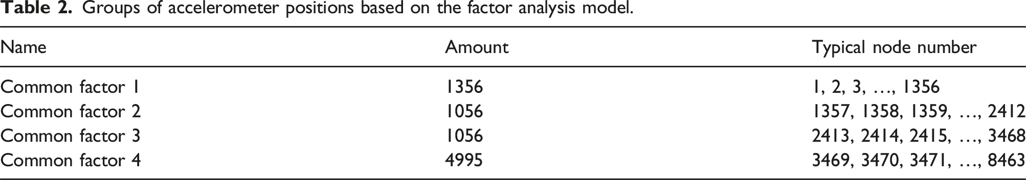
Groups of accelerometer positions based on the factor analysis model.
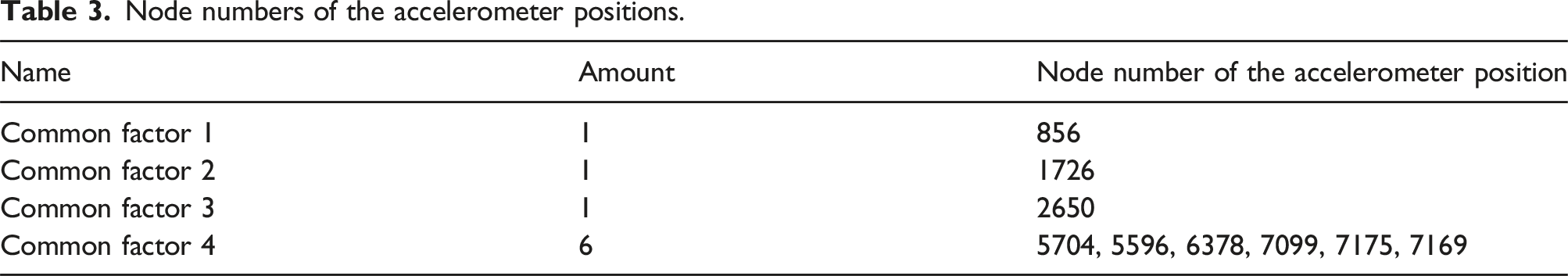
Node numbers of the accelerometer positions.
Results and discussion
Comparison between automatic optimization and uniform distribution schemes
Considering the radiation area and the directivity, the accelerometer positions are generally arranged uniformly on the cylindrical shell, that is, node4009 and node5445 are arranged on one side of the segment cylindrical shell, while node6764 and node7978 are symmetrically arranged on the other side of the segment cylindrical shell as shown in Figure 5(a1) (hereinafter referred to as Scheme 1).
Through an automatic search for optimizing of accelerometer positions, the minimum number of monitoring positions is obtained, that is, node5704, node6378, node7169, and node7175 are all arranged on the cylindrical shell as shown in Figure 5(a2) (hereinafter referred to as Scheme 2).
Considering the measurement position selection and the generalization of the full-domain acoustic inversion, nodes other than the monitoring positions, such as Test_node4297, Test_node4951, Test_node6980, and Test_node8338, are arbitrarily selected as the comparison positions to validate the accuracy of the acoustic reconstruction on the cylindrical shells as shown in Figure 5 (a3). It is worth noting that Test_node4297, Test_node4951, Test_node6980, and Test_node8338 are defined as acoustic inversion positions. The principle of random selection is staying away from the vibration accelerometers known as monitoring positions. When reaching the observation positions, the selection is made on the cylindrical shell with a larger radiation area and where the radiation directionality is more consistent.
As shown in Figure 4, comparing the two schemes with the simulation results, it is found that the response of Scheme 2 has a higher degree of conformity with the simulation results. Scheme 1 exhibits anti-resonance peaks in some areas, such as Test_node8338 at 88 Hz, 132 Hz, and 182 Hz. (a) Schematic layout of measurement and comparison positions of scheme 1 and 2; Comparison of acoustic reconstructions for (b) Test_node4297, (c) Test_node4951, (d) Test_node6980, and (e) Test_node8338.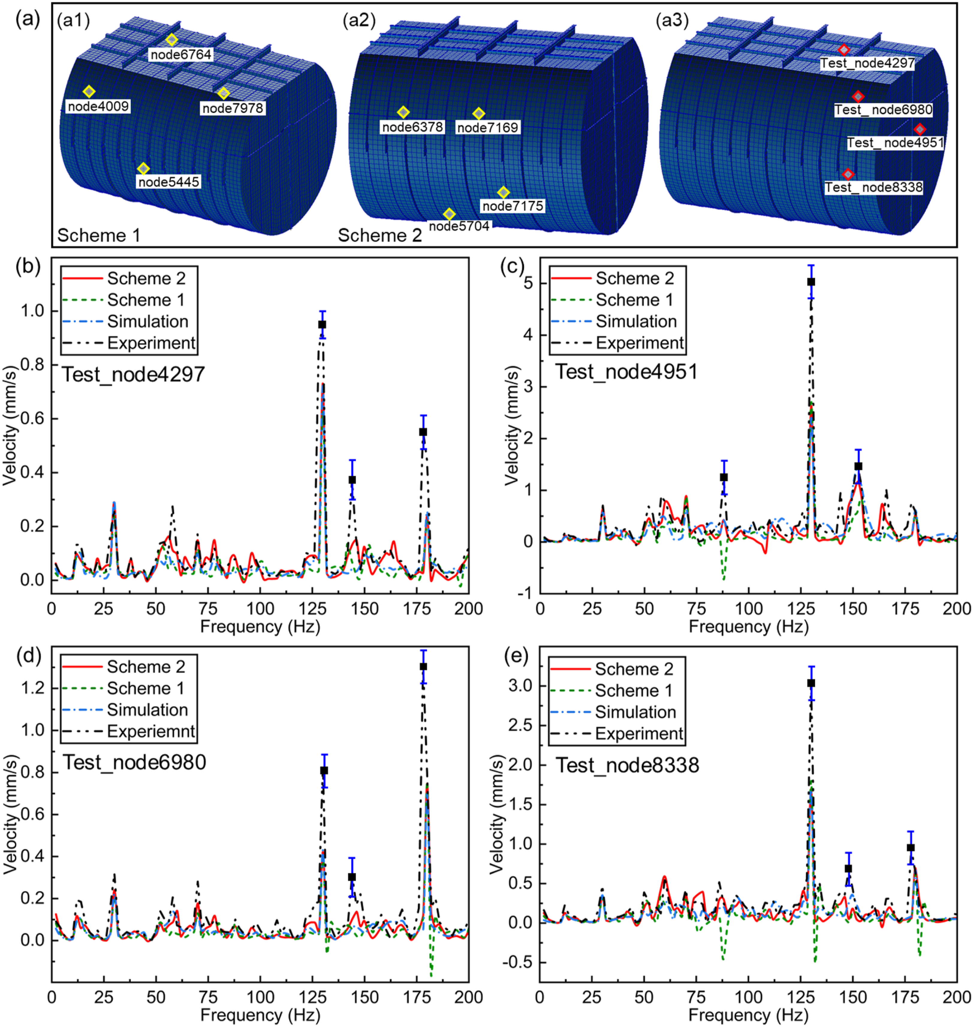
Comparing the two schemes with the experimental results, the main characteristic frequencies of the acoustic inversion can be correctly identified. However, the amplitude at the main characteristic frequencies of the actual measured data is much larger than that of the acoustic inversion and the simulation response. In the experimental environment, the exciter and the base are in surface contact, which results in a greater input of energy to the base and thus leads to a larger response. Additionally, the structural damping in the simulation model may be too small, and the actual value of structural damping is difficult to measure and evaluate.
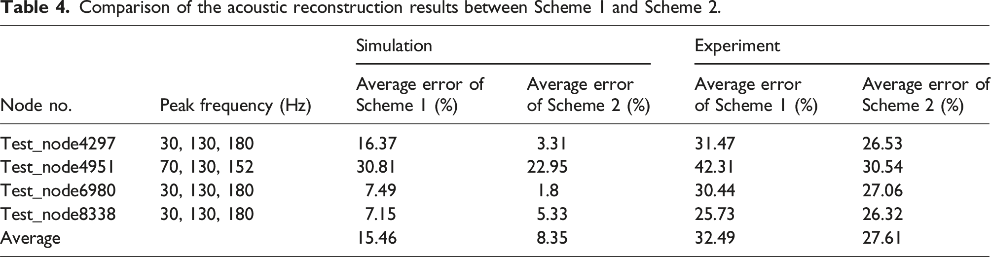
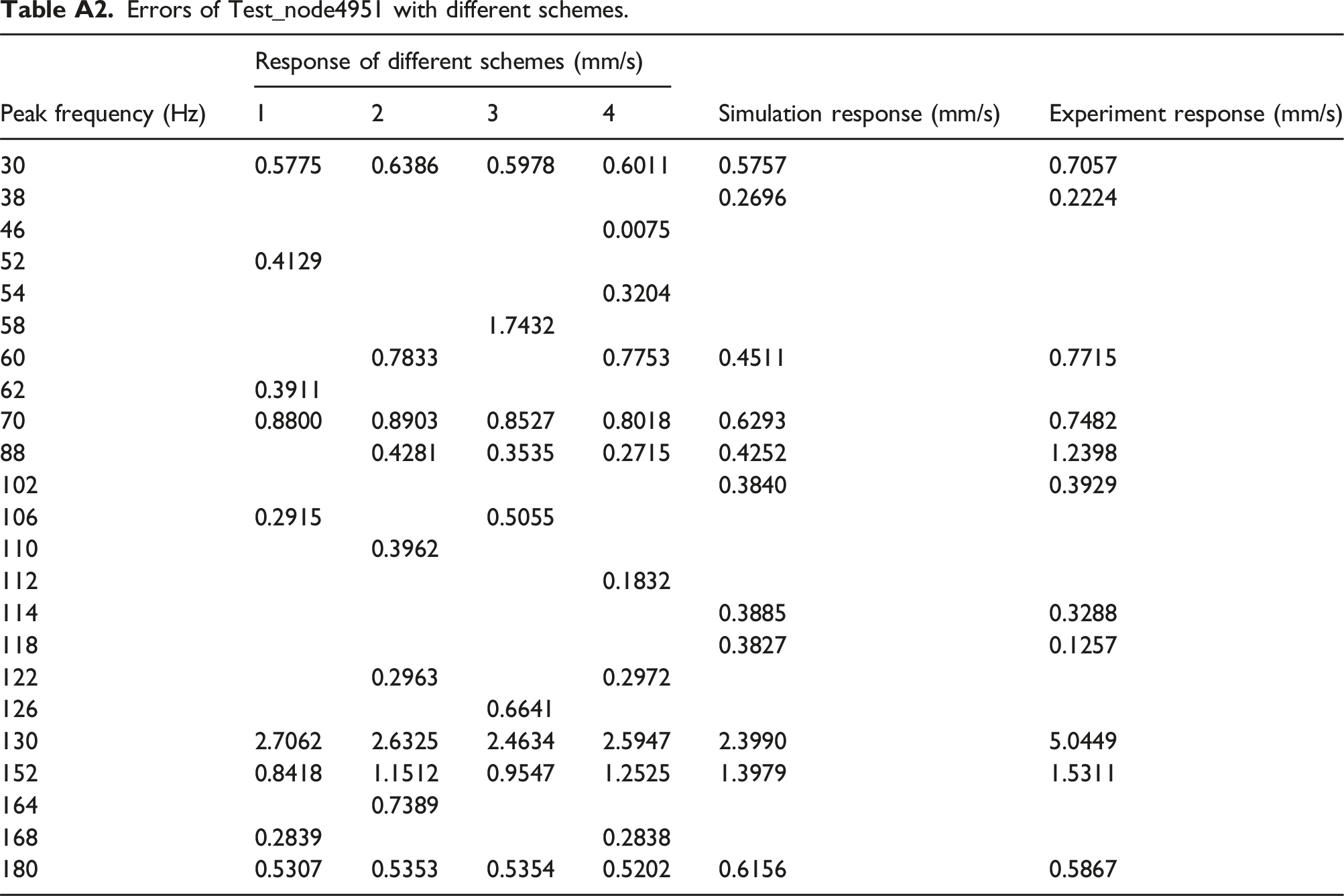
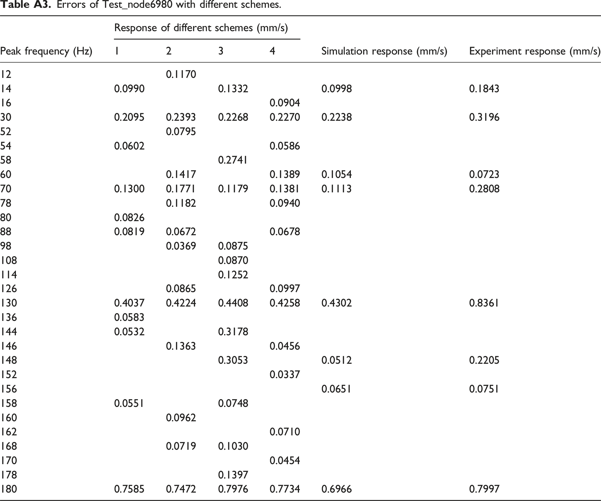
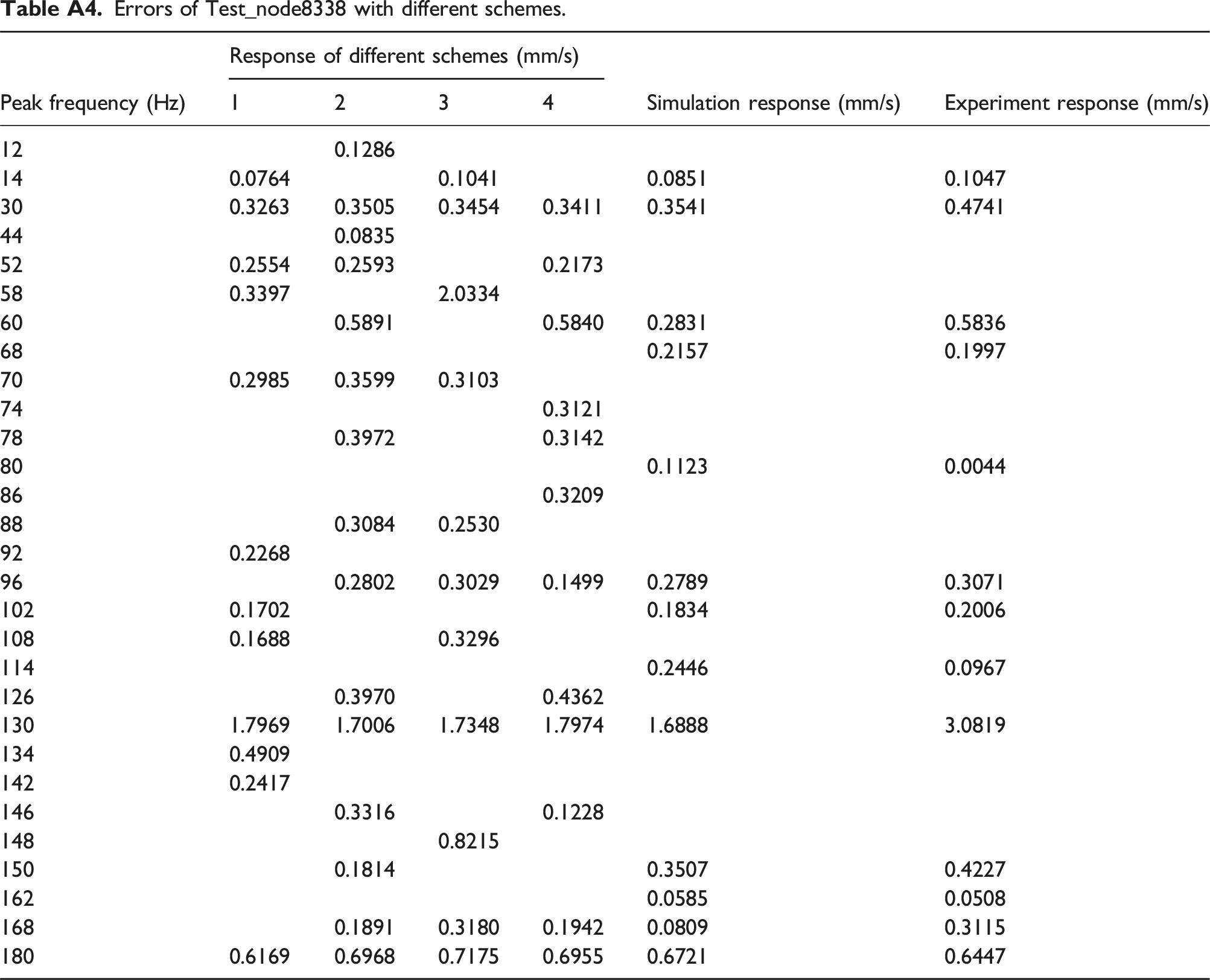
To quantitatively analyze the errors of the two schemes, the response errors of the three characteristic peaks with the highest energy at all nodes are statistically analyzed (for specific statistical data, see the appendix), as shown in Table 3.
The average error of the acoustic reconstruction compared to the simulation at the main characteristic frequencies is almost halved in Scheme 2 compared to Scheme 1. When comparing the acoustic reconstruction to the experiment at main characteristic frequencies, Scheme 2 also shows a slight improvement over Scheme 1 in terms of average errors.
Regardless of simulation or experiment, the errors of Scheme 2 at the four nodes is always less than those of Scheme 1, which directly indicates the great advantages of the automatic optimization method for measurement positions.
Additionally, the error under experimental conditions is greater than the error under simulation conditions. This is because the degree of model refinement leads to discrepancies between the transfer functions of the actual compartment and the simulation model. Furthermore, the lower space of the actual compartment is equipped with ballast iron blocks, which makes it difficult to accurately simulate the real mass distribution in the simulation model.
Comparison of the acoustic reconstruction results between Scheme 1 and Scheme 2.
Comparison between semi-automatic optimization and uniform distribution schemes
Selecting accelerometer positions in different common factor categories can be considered as a semi-automatic optimization method. For example, select node 1726 in common factor 2, node 2650 in common factor 3, and nodes 5596 and 7175 in common factor 4, as shown in Figure 5(a2) (hereinafter named as Scheme 3). Additionally, Scheme 1 and the positions used for validation are shown in Figures 5 (a1) and (a3), respectively. (a) Schematic layout of measurement and comparison positions of Schemes 1 and 3; Comparison of acoustic reconstructions for (b) Test_node4297, (c) Test_node4951, (d) Test_node6980, and (e) Test_node8338.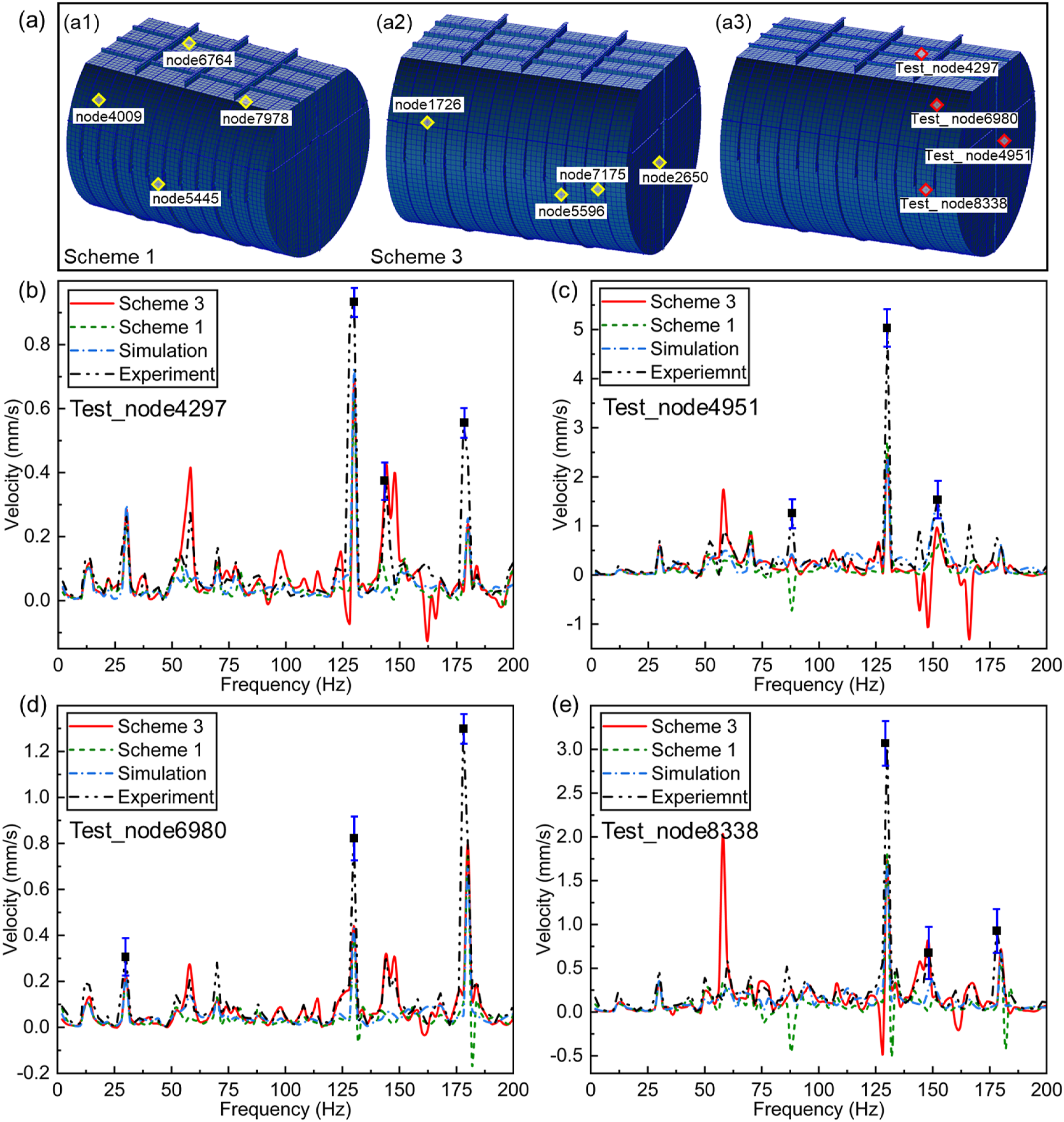
Figures 5(b)–(e) presents the response of four arbitrarily selected nodes under Scheme 1, Scheme 3, and the measured responses.
Overall, the responses obtained for both schemes generally agree with the test responses. Compared to Scheme 1, the curves of Scheme 3 are in better agreement with the measured response, especially at several eigen peaks of higher energy. For instance, for Test_node4297 (see Figure 6(b)), the prediction accuracy of scheme 3 is higher than that of scheme 1 at 30 Hz, 130 Hz, and 180 Hz. However, anomalous eigen-peaks appear in Scheme 3, such as 58 Hz, 144 Hz, 148 Hz in Figure 5(b); 58 Hz, 148 Hz, 166 Hz in Figure 5(c); 58 Hz, 144 Hz, 148 Hz in Figure 5(d); and 58 Hz, 128 Hz, 148 Hz in Figure 5(e). These eigen peaks are mostly the highest peaks or the second-highest peaks in the curve, similar to strong noise interference, which can seriously affect the spectral characteristics of the acoustic reconstruction. To analyze the errors of the two schemes quantitatively, the response errors at the three eigen-peaks with the highest energy of all nodes are counted (see Appendix for specific statistics), as shown in Table 5. (a) Schematic layout of measurement and comparison positions of schemes 2 and 4; Comparison of acoustic reconstructions for (b) Test_node4297, (c) Test_node4951, (d) Test_node6980, and (e) Test_node8338. Comparison of acoustic reconfiguration results for Scheme 1 and Scheme 3.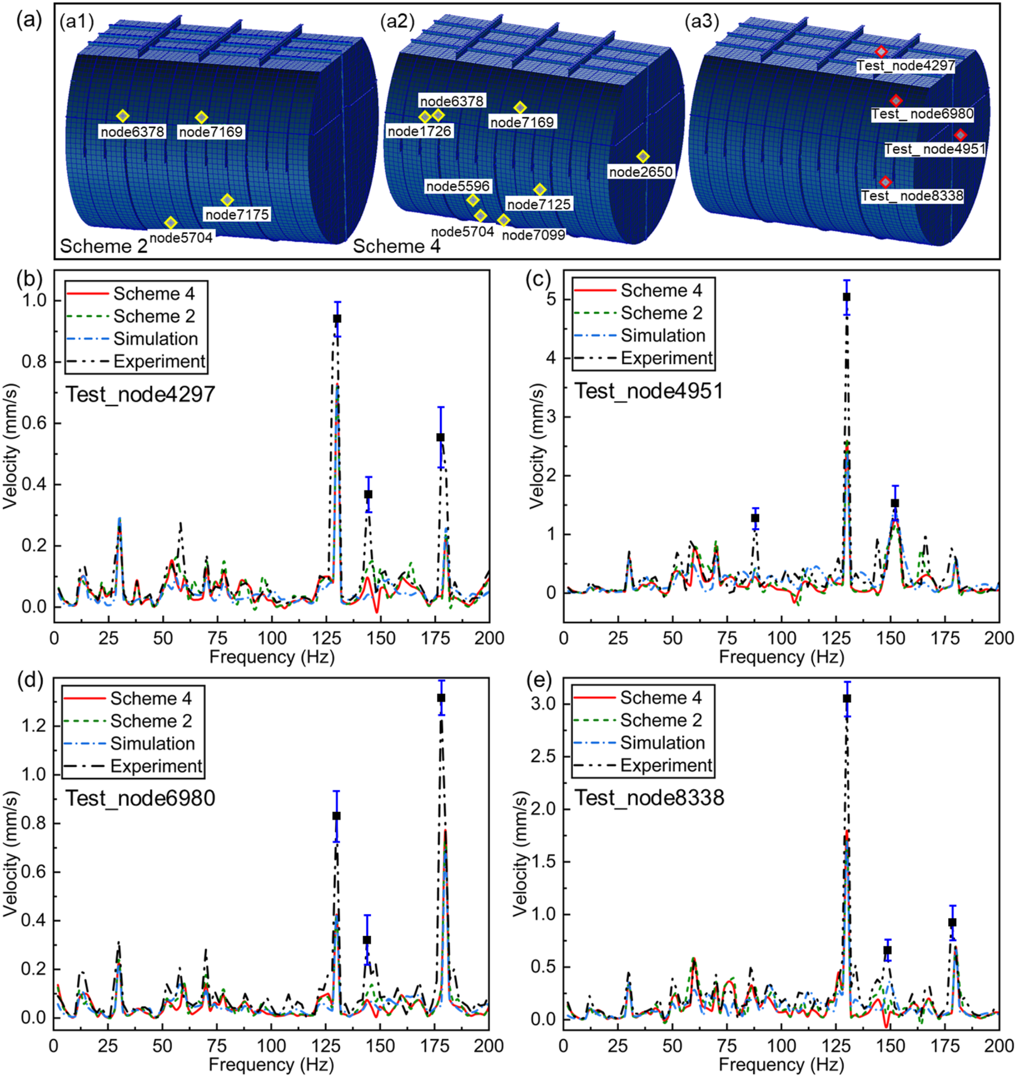
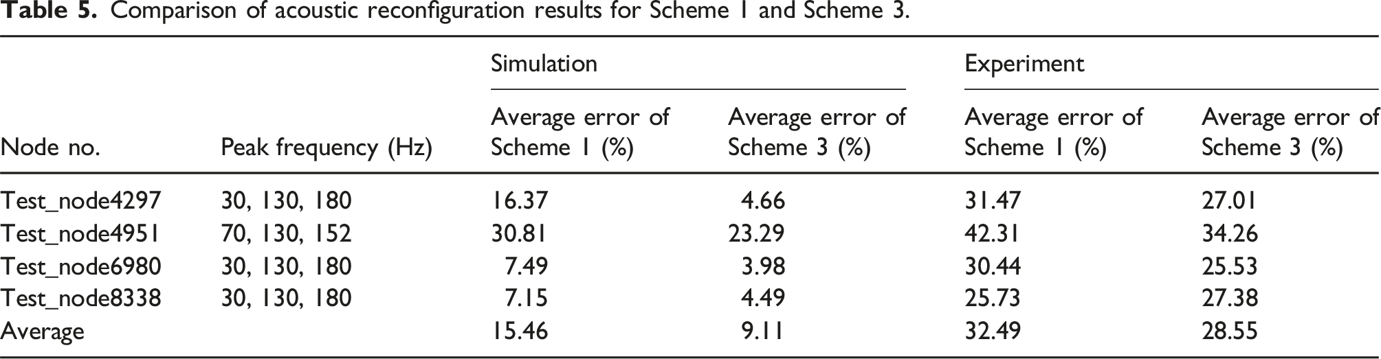
As Table 5 shows, when only characteristic peaks are focused, the error of Scheme 3 is always less than that of Scheme 1 for all four nodes in simulated and experimental scenarios. However, the correlation coefficient over the entire frequency range has decreased. The reason for the decrease in correlation for Scheme 3 is that the introduction of monitoring position data under other common factors are inputted for acoustic reconstruction. However, the data from other categories indicate that the monitoring data itself is diverse, which means noise from other frequencies for acoustic reconstruction is introduced. Therefore, in the process of acoustic reconstruction, through factor analysis, it is preferable to select nodes in the same factor group as the reconstruction position to be vibration monitoring positions.
Comparison of automatic optimization schemes for multiple accelerometer positions
Similar to the automatic optimization scheme of Scheme 2, two accelerometer positions are further added to the cylindrical shell (node 5596 and node 7099), as shown in Figure 6(a2) (hereafter referred to as Scheme 4). Besides, Scheme 2 and the response positions used for validation are shown in Figures 6 (a1) and (a3), respectively.
Comparison of acoustic reconfiguration results for Schemes 2 and 4.
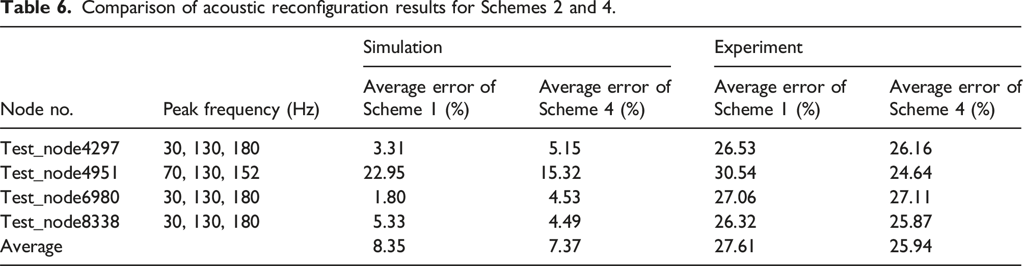
It can be seen from Table 6 that Scheme 4 yields a smaller error. The more stable predictive accuracy is, the more accurate predictive results are. Comparing the simulation with the experiment, the average error of Scheme 4 for the four response positions is slightly less than that of Scheme 2, which indicates that Scheme 4 is more reasonable. Therefore, based on the combined automatic optimization method proposed in this work, selecting more monitoring positions can further improve the accuracy of acoustic reconstruction.
Comparison of the relevance of different schemes
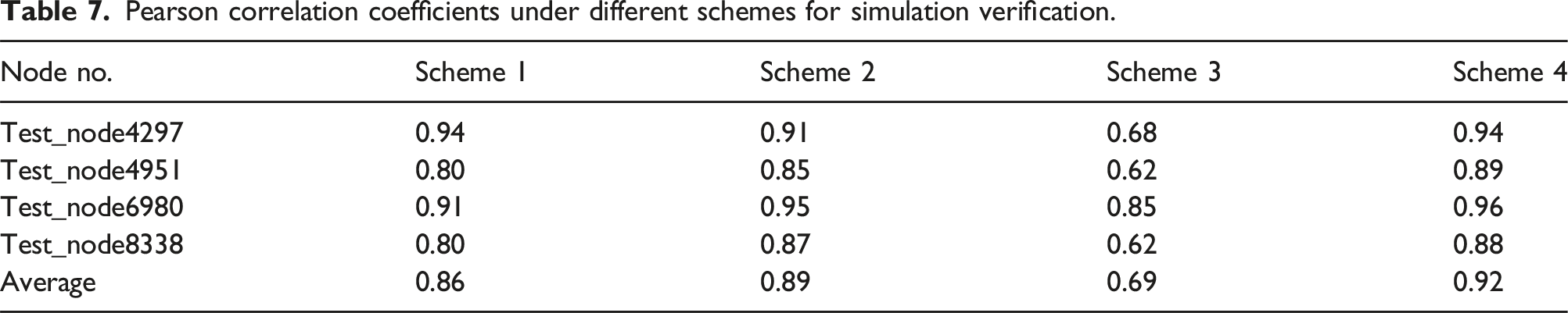
Pearson correlation coefficients under different schemes for simulation verification.
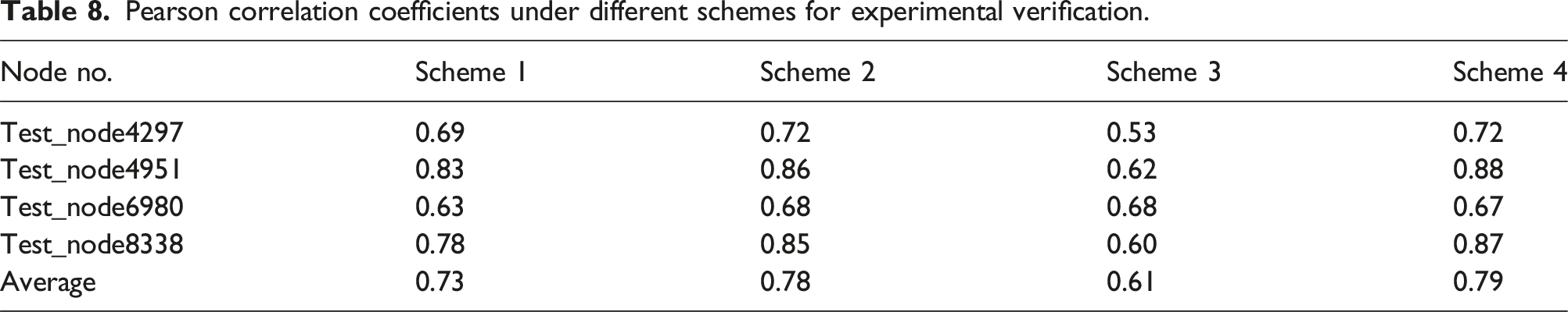
Pearson correlation coefficients under different schemes for experimental verification.
For simulation models, the automatic optimization scheme has improved the correlation coefficient compared to the uniform layout scheme. When the monitoring positions are selected in different groups from the target positions, the correlation coefficient is significantly reduced. The multi-monitoring position automatic optimization scheme yields the best overall curve correlation among these schemes.
The experimental test results are close to the simulation results. In addition, the correlation coefficient of the experimental multi-monitoring position automatic optimization scheme is still close to 0.8 under the interference of various factors such as model errors, excitation errors, and environmental noise, which implies a great potential for engineering applications.
This work addresses the increasing demand for precise vibration monitoring in acoustic control domain, where traditional methods often lack accuracy and reliability. By employing statistical techniques and factor analysis, the study enhances sensor placement strategies, improving measurement accuracy and reducing reconstruction errors. The proposed methodology surpasses engineering requirements for effective noise monitoring in cabin applications. Additionally, the combination of simulation and empirical validation reinforces the robustness of the results, confirming the practical applicability of the optimized sensor configuration.
Conclusions
This work innovatively employs factor analysis to the automatic optimization of accelerometer positions in ship acoustic reconstruction. By achieving data dimensionality reduction through factor analysis and combining them with a multi-criteria evaluation method to provide the best monitoring position layout strategy, the accuracy and efficiency of acoustic reconstruction are improved. Simulated and experimental verification are conducted on a cabin segment, and the error of acoustic reconstruction are utilized as the evaluation index for the selection of monitoring positions. The following conclusions are drawn: (1) In simulated verification, at the main peak frequency, the error via automatic optimization measurement positions is significantly reduced from 15.46% to 8.35% compared to the uniform distribution method, and the correlation coefficient is also improved from 0.86 to 0.89. (2) In simulated verification, the semi-automatic optimization method, shows a decrease in the correlation coefficient from 0.86 to 0.69 compared to the uniform distribution method. This indicates that selecting accelerometers from other factor groups as inputs in the acoustic reconstruction process will harm acoustic reconstruction. (3) In simulated verification, based on the automatic optimization method, the error is further reduced from 8.35% to 7.37%, and the correlation is improved from 0.89 to 0.92 by adding more measurement positions, which enhances both accuracy and correlation. (4) The conclusions from experimental verification are similar to those from the above three simulation verifications. Additionally, after adding more measurement positions based on the automatic optimization method, the correlation coefficient between acoustic reconstruction and actual measured data is close to 0.8, indicating that this method is valuable for further engineering applications. In addition, the robustness and accuracy of the accelerometer optimization method proposed in this paper need to be further improved.
Footnotes
Declaration of conflicting interests
The author(s) declared no potential conflicts of interest with respect to the research, authorship, and/or publication of this article.
Funding
The author(s) disclosed receipt of the following financial support for the research, authorship, and/or publication of this article: This work was gratefully supported by the National Natural Science Foundation of China (52305110) and the Ministry of Industry and Information Technology’s “High Technology Ship Research Project, China” (Ministry of Industry and Information Technology MC-201918-C10).
Acoustic reconstruction errors at different nodes
Errors of Test_node4297 with different schemes. Errors of Test_node4951 with different schemes. Errors of Test_node6980 with different schemes. Errors of Test_node8338 with different schemes.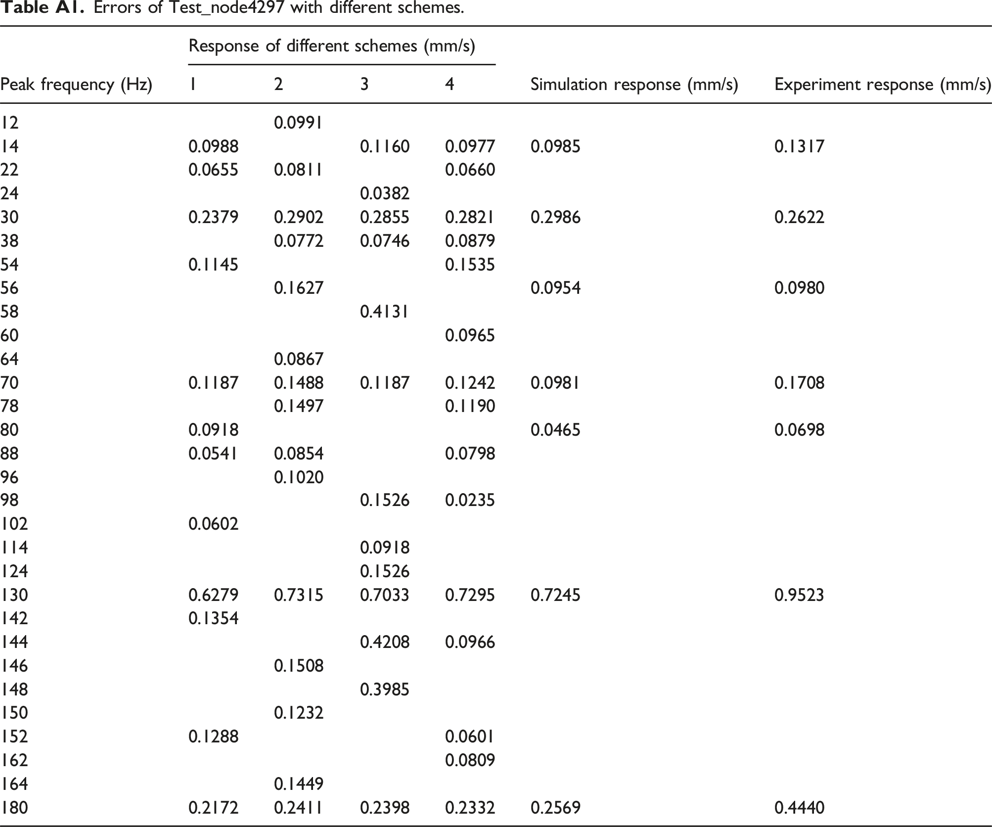
Peak frequency (Hz)
Response of different schemes (mm/s)
Simulation response (mm/s)
Experiment response (mm/s)
1
2
3
4
12
0.0991
14
0.0988
0.1160
0.0977
0.0985
0.1317
22
0.0655
0.0811
0.0660
24
0.0382
30
0.2379
0.2902
0.2855
0.2821
0.2986
0.2622
38
0.0772
0.0746
0.0879
54
0.1145
0.1535
56
0.1627
0.0954
0.0980
58
0.4131
60
0.0965
64
0.0867
70
0.1187
0.1488
0.1187
0.1242
0.0981
0.1708
78
0.1497
0.1190
80
0.0918
0.0465
0.0698
88
0.0541
0.0854
0.0798
96
0.1020
98
0.1526
0.0235
102
0.0602
114
0.0918
124
0.1526
130
0.6279
0.7315
0.7033
0.7295
0.7245
0.9523
142
0.1354
144
0.4208
0.0966
146
0.1508
148
0.3985
150
0.1232
152
0.1288
0.0601
162
0.0809
164
0.1449
180
0.2172
0.2411
0.2398
0.2332
0.2569
0.4440
Peak frequency (Hz)
Response of different schemes (mm/s)
Simulation response (mm/s)
Experiment response (mm/s)
1
2
3
4
30
0.5775
0.6386
0.5978
0.6011
0.5757
0.7057
38
0.2696
0.2224
46
0.0075
52
0.4129
54
0.3204
58
1.7432
60
0.7833
0.7753
0.4511
0.7715
62
0.3911
70
0.8800
0.8903
0.8527
0.8018
0.6293
0.7482
88
0.4281
0.3535
0.2715
0.4252
1.2398
102
0.3840
0.3929
106
0.2915
0.5055
110
0.3962
112
0.1832
114
0.3885
0.3288
118
0.3827
0.1257
122
0.2963
0.2972
126
0.6641
130
2.7062
2.6325
2.4634
2.5947
2.3990
5.0449
152
0.8418
1.1512
0.9547
1.2525
1.3979
1.5311
164
0.7389
168
0.2839
0.2838
180
0.5307
0.5353
0.5354
0.5202
0.6156
0.5867
Peak frequency (Hz)
Response of different schemes (mm/s)
Simulation response (mm/s)
Experiment response (mm/s)
1
2
3
4
12
0.1170
14
0.0990
0.1332
0.0998
0.1843
16
0.0904
30
0.2095
0.2393
0.2268
0.2270
0.2238
0.3196
52
0.0795
54
0.0602
0.0586
58
0.2741
60
0.1417
0.1389
0.1054
0.0723
70
0.1300
0.1771
0.1179
0.1381
0.1113
0.2808
78
0.1182
0.0940
80
0.0826
88
0.0819
0.0672
0.0678
98
0.0369
0.0875
108
0.0870
114
0.1252
126
0.0865
0.0997
130
0.4037
0.4224
0.4408
0.4258
0.4302
0.8361
136
0.0583
144
0.0532
0.3178
146
0.1363
0.0456
148
0.3053
0.0512
0.2205
152
0.0337
156
0.0651
0.0751
158
0.0551
0.0748
160
0.0962
162
0.0710
168
0.0719
0.1030
170
0.0454
178
0.1397
180
0.7585
0.7472
0.7976
0.7734
0.6966
0.7997
Peak frequency (Hz)
Response of different schemes (mm/s)
Simulation response (mm/s)
Experiment response (mm/s)
1
2
3
4
12
0.1286
14
0.0764
0.1041
0.0851
0.1047
30
0.3263
0.3505
0.3454
0.3411
0.3541
0.4741
44
0.0835
52
0.2554
0.2593
0.2173
58
0.3397
2.0334
60
0.5891
0.5840
0.2831
0.5836
68
0.2157
0.1997
70
0.2985
0.3599
0.3103
74
0.3121
78
0.3972
0.3142
80
0.1123
0.0044
86
0.3209
88
0.3084
0.2530
92
0.2268
96
0.2802
0.3029
0.1499
0.2789
0.3071
102
0.1702
0.1834
0.2006
108
0.1688
0.3296
114
0.2446
0.0967
126
0.3970
0.4362
130
1.7969
1.7006
1.7348
1.7974
1.6888
3.0819
134
0.4909
142
0.2417
146
0.3316
0.1228
148
0.8215
150
0.1814
0.3507
0.4227
162
0.0585
0.0508
168
0.1891
0.3180
0.1942
0.0809
0.3115
180
0.6169
0.6968
0.7175
0.6955
0.6721
0.6447