Sage Journals: Discover world-class research

Abstract

The nonlinear energy sink is a nonlinear shock absorber that provides targeted energy transfer and plays a crucial role in structural vibration suppression. In this paper, the energy transfer and dynamic characteristics of nonlinear damping nonlinear energy sink systems are analyzed. Firstly, the theoretical model of the nonlinear damping NES system is described, and secondly, the equations of the system in the free state are derived by using the complex variable average method and the multi-scale method to obtain the energy transfer efficiency equation of the system. Through the study of the slow invariant manifold and energy transfer efficiency of the system, the influence of each system parameter on the energy transfer efficiency is analyzed. Then the equations of the system under harmonic excitation are processed in the same method to obtain the boundary equations of the system, through which the saddle-node bifurcation diagram of the system is plotted to study the influence of each system parameter on the saddle-node bifurcation characteristics of the system. Finally, the slow-varying equation of the system under harmonic excitation is derived, and the influence of each system parameter on the frequency detuning parameter interval of the strongly modulated response is obtained using the phase trajectory and a one-dimensional mapping diagram of the system, and the time-mileage diagram and Poincare section are used to prove the damping effect of the strongly modulated response.

Keywords

Nonlinear energy sink complex variable average method strongly modulated response saddle-node bifurcation

Introduction

With the problem of nonlinear vibration becoming more and more prominent, traditional linear damping devices can not satisfy practical needs in engineering. In this engineering background, nonlinear vibration damping devices with geometrical structures have emerged.^1–4 Among them, nonlinear energy sink (NES) is a special nonlinear vibration damping device, which consists of a small mass block, viscous damping and a strong nonlinear spring.^5–7 Under certain initial energy conditions, a special energy absorption mechanism appears, which is called targeted energy transfer (TET), and it can realize unidirectional irreversible energy transfer.^8–10 Under harmonic excitation, an NES system can show a reciprocating and continuous nonlinear unidirectional energy transfer phenomenon, known as strongly modulated response (SMR).^11,12 Because the NES has a wide vibration absorption band, and excellent vibration damping characteristics and robustness, it has been extensively studied. As a result, many new NES structures have been proposed, including lever-type NES, track NES, non-smooth NES, and bistable NES structures.^13–15

Studying the energy transfer efficiency of an NES can intuitively describe the vibration reduction effect of the NES on the primary system. Nguyen et al¹⁶ analyzed the effect of NES stiffness and mass on the energy transfer efficiency by means of energy change curves, and obtained the minimum stiffness of a single degree of freedom NES to achieve target energy transfer. Gourdon et al¹⁷ analyzed the phenomenon of target energy transfer occurring in NES under different kinds of excitations and found that when the amplitude of the external excitation is in a suitable range, the system shows a quasi-periodic response. Zhang et al¹⁸ used a numerical method to study the energy changes of wing coupled conventional NES, pointing out the effects of different wing states on the energy transfer efficiency of NES. AL-Shudeifat¹⁹ proposed a new time-varying stiffness method and used it to study the effect of initial energy on energy transfer.

Strongly modulated response is one of the manifestations of the vibration suppression capability of the NES. Gendelman et al^12,20,21 analyzed this special response by means of complex variable average method and found that this special response is formed when the primary system and the NES have 1:1 resonance. Subsequently, scholars have tried to use various methods to analyze whether the SMR occurs in the system and the conditions under which it occurs, and Starosvetsky et al^22,23 used the multi-scale method to make a further analysis, and found that the system can produce SMR only if it contains a nonlinear component. Kong et al²⁴ also found that the presence of SMR is affected by the frequency detuning parameter after their study, but did not reveal the law of influence.

In order to solve the above problems, this paper firstly construct a nonlinear damping NES system model from the perspective of approximate analysis, and derives the slow invariant manifold and the energy transfer efficiency equation to deeply study the influence of each system parameter on the energy transfer efficiency. Secondly, the number of equilibrium points of the system is investigated by using the saddle-node bifurcation equation, and the effects of different detuning parameters, cubic stiffness coefficients, and mass ratios on the boundary of the saddle-node bifurcation are revealed. Finally, the necessary conditions for SMR generation are investigated by phase trajectory and one-dimensional mapping, and the effects of external excitation amplitude, nonlinear damping coefficients and cubic stiffness coefficients on the existence of detuning parameter intervals of SMR are analyzed, which provide some reference for the parameter design of NES.

Model statement of structure-nonlinear damping NES system

The model of a nonlinear damping NES system is composed of two main parts: the primary system and the nonlinear damping NES. The primary system consists of a mass block, linear spring, and linear damping. The nonlinear damping NES consists of a small mass block, nonlinear spring, and nonlinear damping. The nonlinear damping NES system model is shown in Figure 1.

where $m_{1}$ and $m_{2}$ are the masses of the primary system and nonlinear damping NES, respectively; $c_{1}$ and $c_{2}$ are the damping of the primary system and nonlinear damping NES, respectively; $k_{1}$ and $k_{2}$ are the linear stiffness and nonlinear stiffness, respectively; and $x_{1}$ and $x_{2}$ are the displacements of the primary system and nonlinear damping NES, respectively. $F$ and $Ω$ are the amplitude and frequency of forced excitation, respectively. Using Newton’s law, the dynamic motion of the nonlinear damping NES system is given by

{\begin{cases} m_{1} {\ddot{x}}_{1} + c_{1} {\dot{x}}_{1} + k_{1} x_{1} + c_{2} {({\dot{x}}_{1} - {\dot{x}}_{2})}^{3} + k_{2} {(x_{1} - x_{2})}^{3} = F \cos (Ω T) \\ m_{2} {\ddot{x}}_{2} + c_{2} {({\dot{x}}_{2} - {\dot{x}}_{1})}^{3} + k_{2} {(x_{2} - x_{1})}^{3} = 0 \end{cases}

(1)

Figure 1.

Dynamic model of the nonlinear damping NES system.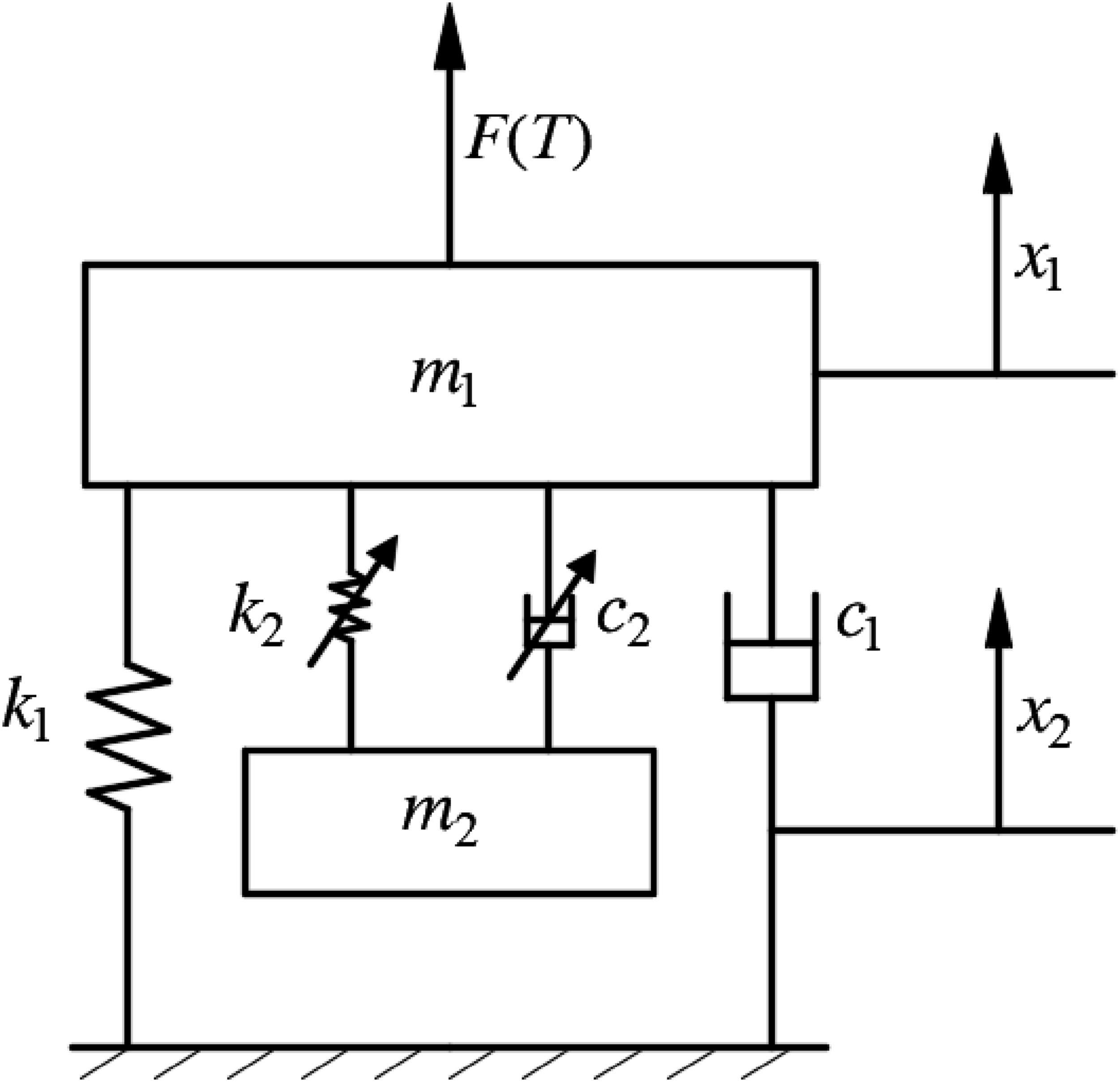

Analysis of energy transfer characteristics

Solve the system slow-varying equation

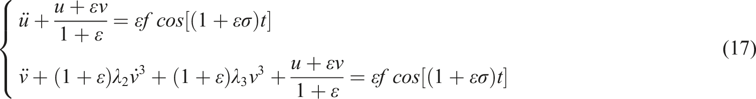
Since the energy transfer efficiency is only related to the structural parameters of the system, which have nothing to do with harmonic excitation, the free state of the nonlinear damping NES system is studied. Equation (1) then takes the form

{\begin{cases} m_{1} {\ddot{x}}_{1} + c_{1} {\dot{x}}_{1} + k_{1} x_{1} + c_{2} {({\dot{x}}_{1} - {\dot{x}}_{2})}^{3} + k_{2} {(x_{1} - x_{2})}^{3} = 0 \\ m_{2} {\ddot{x}}_{2} + c_{2} {({\dot{x}}_{2} - {\dot{x}}_{1})}^{3} + k_{2} {(x_{2} - x_{1})}^{3} = 0 \end{cases}

(2)

To facilitate obtaining a solution to equation (2) the following variables are used

ε = \frac{m_{2}}{m_{1}} < < 1, ε λ_{1} = \frac{c_{1}}{m_{1}}, ε λ_{2} = \frac{c_{2}}{m_{1}}, ω^{2} = \frac{k_{1}}{m_{1}}, ε λ_{3} = \frac{k_{2}}{m_{1}}

where ε is the mass ratio of the nonlinear damping NES to the primary system; ω is the natural frequency of system.

After a change of variables, the system can be described by

{\begin{cases} {\ddot{x}}_{1} + ε λ_{1} {\dot{x}}_{1} + ω^{2} x_{1} + ε λ_{2} {({\dot{x}}_{1} - {\dot{x}}_{2})}^{3} + ε λ_{3} {(x_{1} - x_{2})}^{3} = 0 \\ ε {\ddot{x}}_{2} + ε λ_{2} {({\dot{x}}_{2} - {\dot{x}}_{1})}^{3} + ε k_{3} {(x_{2} - x_{1})}^{3} = 0 \end{cases}

(3)

Using the change of state variables $u = x_{1}$ and $w = x_{2} - x_{1}$ , equation (3) can be reduced to

{\begin{cases} (1 + ε) \ddot{u} + ε \ddot{w} + ε λ_{1} \dot{u} + ω^{2} u = 0 \\ ε (\ddot{u} + \ddot{w}) + ε λ_{2} {\dot{w}}^{3} + ε λ_{3} w^{3} = 0 \end{cases}

(4)

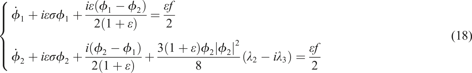
Because the energy transfer is dominated by the 1:1 internal resonance of the system, this paper focuses on the energy transfer arising from this resonance. The imaginary part coefficient of the complex variable is ω. Then, introducing the complex variables $ϕ_{1} e^{i ω t} = \dot{u} + i ω u$ , $ϕ_{2} e^{i ω t} = \dot{w} + i ω w$ , equation (4) can be rewritten as

{\begin{cases} (1 + ε) {\dot{ϕ}}_{1} + ε {\dot{ϕ}}_{2} + \frac{ε}{2} i ω (ϕ_{1} + ϕ_{2}) + \frac{ε}{2} λ_{1} ϕ_{1} = 0 \\ {\dot{ϕ}}_{1} + {\dot{ϕ}}_{2} + \frac{1}{2} i ω (ϕ_{1} + ϕ_{2}) + \frac{3 λ_{2}}{8} ϕ_{2} {| ϕ_{2} |}^{2} - \frac{3 i λ_{3}}{8 ω^{3}} ϕ_{2} {| ϕ_{2} |}^{2} = 0 \end{cases}

(5)

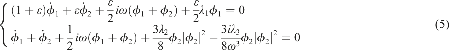
Since the above equations contain nonlinear terms, it is impossible to obtain accurate analytical solutions. Therefore, it is necessary to solve by the multi-scale method. The time scale introduced is $ϕ_{j} = ϕ_{j 0} + ε ϕ_{j 1}$ , $\forall j = 1, 2$ , $t = t_{0} + t_{1}$ . Equation (5) can be converted to

{\begin{cases} (1 + ε) (\frac{\partial ϕ_{10}}{\partial t_{0}} + ε \frac{\partial ϕ_{10}}{\partial t_{1}} + ε \frac{\partial ϕ_{11}}{\partial t_{0}} + ε^{2} \frac{\partial ϕ_{11}}{\partial t_{1}}) + ε (\frac{\partial ϕ_{20}}{\partial t_{0}} + ε \frac{\partial ϕ_{20}}{\partial t_{1}} + ε \frac{\partial ϕ_{21}}{\partial t_{0}} + {ε_{0}}^{2} \frac{\partial ϕ_{21}}{\partial t_{1}}) \\ + \frac{ε}{2} i ω (ϕ_{10} + ε ϕ_{11} + ϕ_{20} + ε ϕ_{21}) + \frac{ε}{2} λ_{1} (ϕ_{10} + ε ϕ_{11}) = 0 \\ (\frac{\partial ϕ_{10}}{\partial t_{0}} + ε \frac{\partial ϕ_{10}}{\partial t_{1}} + ε \frac{\partial ϕ_{11}}{\partial t_{0}} + ε^{2} \frac{\partial ϕ_{11}}{\partial t_{1}} + \frac{\partial ϕ_{20}}{\partial t_{0}} + ε \frac{\partial ϕ_{20}}{\partial t_{1}} + ε \frac{\partial ϕ_{21}}{\partial t_{0}} + ε^{2} \frac{\partial ϕ_{21}}{\partial t_{1}}) + \frac{i ω}{2} (ϕ_{10} + ε ϕ_{11} \\ + ϕ_{20} + ε ϕ_{21}) + \frac{3 λ_{2}}{8} (ϕ_{20} + ε ϕ_{21}) {| ϕ_{20} + ε ϕ_{21} |}^{2} - \frac{3 i λ_{3}}{8 ω^{3}} (ϕ_{20} + ε ϕ_{21}) {| ϕ_{20} + ε ϕ_{21} |}^{2} = 0 \end{cases}

(6)

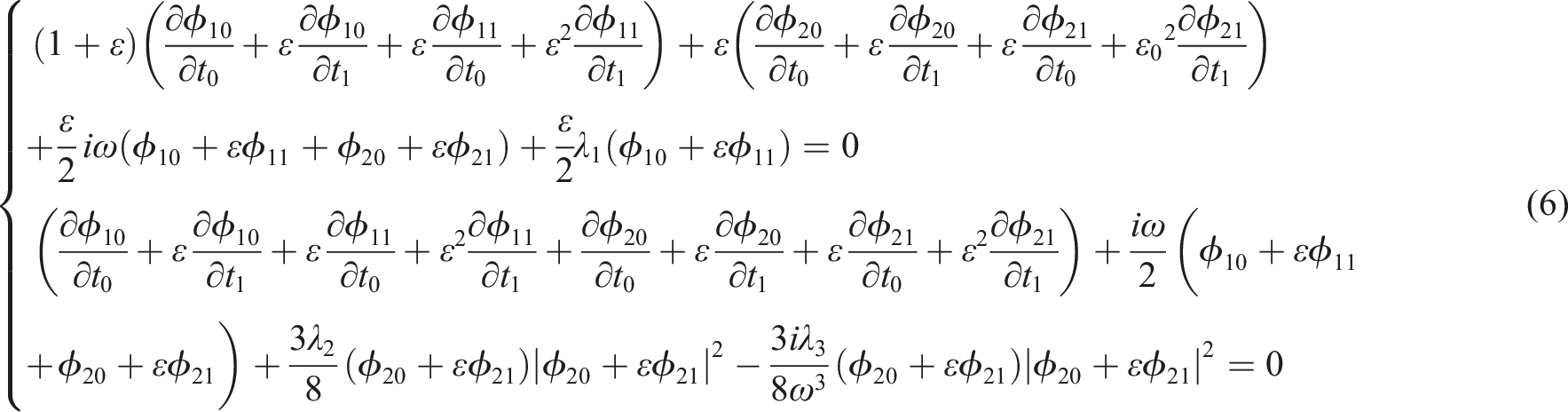
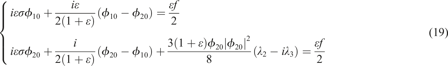
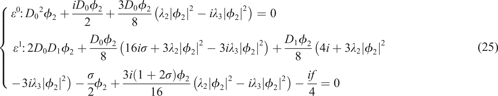
The fast variable part (ε⁰) in equation (6) is expressed as

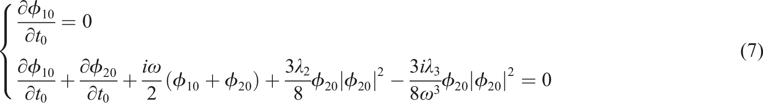
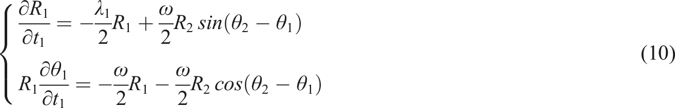
{\begin{cases} \frac{\partial ϕ_{10}}{\partial t_{0}} = 0 \\ \frac{\partial ϕ_{10}}{\partial t_{0}} + \frac{\partial ϕ_{20}}{\partial t_{0}} + \frac{i ω}{2} (ϕ_{10} + ϕ_{20}) + \frac{3 λ_{2}}{8} ϕ_{20} {| ϕ_{20} |}^{2} - \frac{3 i λ_{3}}{8 ω^{3}} ϕ_{20} {| ϕ_{20} |}^{2} = 0 \end{cases}

(7)

The slow variable part (ε¹) in equation (6) is expressed as

\frac{\partial ϕ_{10}}{\partial t_{0}} + \frac{\partial ϕ_{10}}{\partial t_{1}} + \frac{\partial ϕ_{11}}{\partial t_{0}} + \frac{\partial ϕ_{20}}{\partial t_{0}} + \frac{i ω}{2} (ϕ_{10} + ϕ_{20}) + \frac{λ_{1}}{2} ϕ_{10} = 0

(8)

Eq. (7) and Eq. (8) show that

ϕ_{10}

and

ϕ_{20}

depend only on the timescale. Therefore, equation (8) can be rewritten as

\frac{\partial ϕ_{10}}{\partial t_{1}} + \frac{i ω}{2} (ϕ_{10} + ϕ_{20}) + \frac{λ_{1}}{2} ϕ_{10} = 0

(9)

In order to investigate the evolution of the system amplitude, and using the magnitude and phase angle to represent complex variables,

ϕ_{10} = R_{1} (t_{1}) e^{i θ_{1} (t_{1})}

and

ϕ_{20} = R_{2} (t_{1}) e^{i θ_{2} (t_{1})}

. Equation (9) can now be reduced to

{\begin{cases} \frac{\partial R_{1}}{\partial t_{1}} = - \frac{λ_{1}}{2} R_{1} + \frac{ω}{2} R_{2} \sin (θ_{2} - θ_{1}) \\ R_{1} \frac{\partial θ_{1}}{\partial t_{1}} = - \frac{ω}{2} R_{1} - \frac{ω}{2} R_{2} \cos (θ_{2} - θ_{1}) \end{cases}

(10)

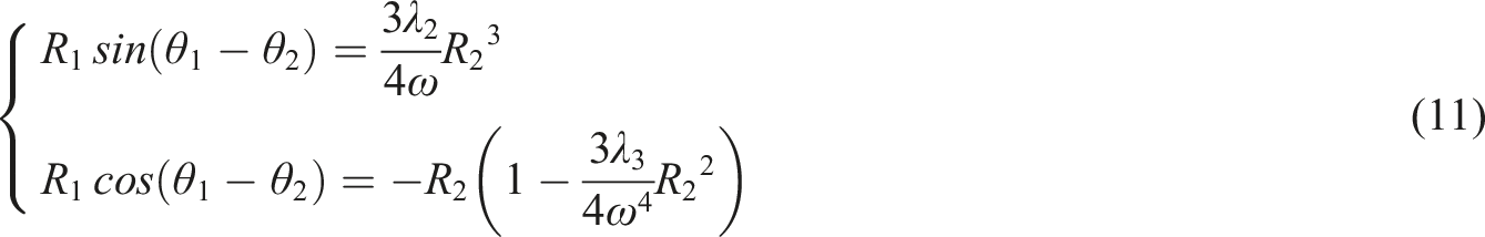
The second equation in the equation (7) can be reduced to

{\begin{cases} R_{1} \sin (θ_{1} - θ_{2}) = \frac{3 λ_{2}}{4 ω} {R_{2}}^{3} \\ R_{1} \cos (θ_{1} - θ_{2}) = - R_{2} (1 - \frac{3 λ_{3}}{4 ω^{4}} {R_{2}}^{2}) \end{cases}

(11)

By combining equations (10) and (11) and using new variables,

E_{1} = {R_{1}}^{2}, E_{2} = {R_{2}}^{2}

, the slow-varying equation of the nonlinear damping NES system is given by

{\begin{cases} \frac{\partial E_{1}}{\partial t_{1}} = - λ_{1} E_{1} - \frac{3 λ_{2}}{4} {E_{2}}^{2} \\ E_{1} = E_{2} [{(\frac{3 λ_{2}}{4 ω} E_{2})}^{2} + {(1 - \frac{3 λ_{3}}{4 ω^{4}} E_{2})}^{2}] \end{cases}

(12)

where E₁ is the first approximation of the primary system energy at multiple scales, and E₂ is the first approximation of the nonlinear damping NES energy at multiple scales. The first formula in equation (12) shows that the partial derivative of the primary system energy is less than or equal to 0 and is constant; therefore, the primary system energy decreases monotonically. The second formula shows that the energy transfer of the nonlinear damping NES system is not only affected by the damping of the NES, but also by the stiffness of the NES.

Slow invariant manifold analysis

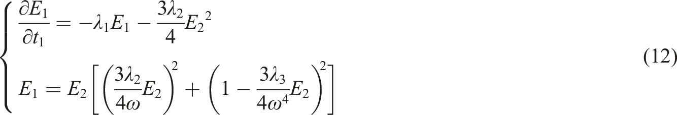
Equation (12) represents the slow invariant manifold; the parameters are selected as λ₂ = 0.2, λ₃ = 1.2, ω = 1, as shown in Figure 2.

Figure 2.

Slow invariant manifold of a nonlinear damping NES system.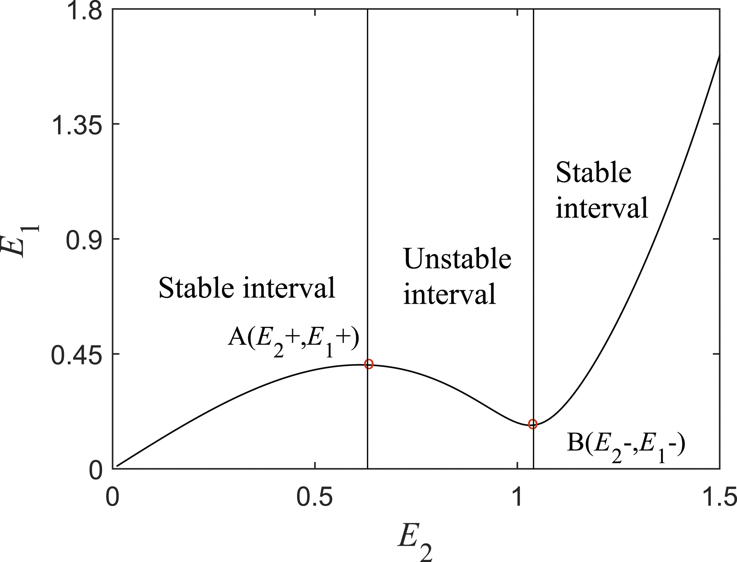

The abscissa in the figure represents the nonlinear damping NES energy, and the ordinate represents the primary system energy. There are two extreme points in the slow invariant manifold diagram of this system, A and B, respectively, which are unstable. The interval between the two vertical lines is an unstable interval, and the other intervals are stable intervals.

Next, the slow invariant manifold comparison diagram between the nonlinear damping NES system and other systems is drawn, the parameter selection is the same as previously, as shown in Figure 3.

Figure 3.

Comparison diagram of slow invariant manifold.

In Figure 3, which under the same parameter selection, the amount of energy required by the nonlinear damping NES system to trigger TET is smaller than that required by the coupled damping NES system and the linear damping NES system. This indicates that the nonlinear damping NES system achieves energy transfer more easily than the other two systems. The difference between the maximum and the minimum of the nonlinear damping NES system is also larger than that of the other two systems. This means that the energy transfer efficiency of the nonlinear damping NES system is higher than that of the other two systems. The relation is as follows

E_{t r N} > E_{t r L} > E_{t r C}

(13)

where E_tr is the energy transfer efficiency.

Energy transfer efficiency analysis

Solving the second equation in equation (12), the coordinates of points A and point B are obtained

\begin{array}{l} {E_{2}}_{+} = \frac{4 ω^{4} (2 λ_{3} - h)}{9 ({λ_{3}}^{2} + {λ_{2}}^{2} ω^{6})} & E_{1 +} = \frac{8 ω^{4} (2 λ_{3} - h) ({λ_{3}}^{2} + 3 {λ_{2}}^{2} ω^{6} + λ_{3} h)}{81 {({λ_{3}}^{2} + {λ_{2}}^{2} ω^{6})}^{2}} \\ {E_{2}}_{-} = \frac{4 ω^{4} (2 λ_{3} + h)}{9 ({λ_{3}}^{2} + {λ_{2}}^{2} ω^{6})} & E_{1 -} = \frac{8 ω^{4} (2 λ_{3} + h) ({λ_{3}}^{2} + 3 {λ_{2}}^{2} ω^{6} - λ_{3} h)}{81 {({λ_{3}}^{2} + {λ_{2}}^{2} ω^{6})}^{2}} \end{array}

where

h = \sqrt{{λ_{3}}^{2} - 3 {λ_{2}}^{2} ω^{6}}

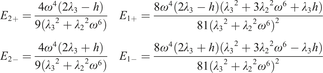
From the coordinates of the extreme points, it can be seen that the two extreme points must satisfy the following conditions

h = \sqrt{{λ_{3}}^{2} - 3 {λ_{2}}^{2} ω^{6}} \geq 0 \Rightarrow ω^{3} λ_{2} \leq \frac{1}{\sqrt{3}} λ_{3}

(14)

The above equation shows that, when the natural frequency of the primary system is constant, the λ₂ and λ₃ must satisfy the conditions, otherwise the system cannot achieve TET. In order to facilitate the analysis, a three-dimensional diagram of the above equation is shown in Figure 4.

Figure 4.

Diagram of TET implementing condition.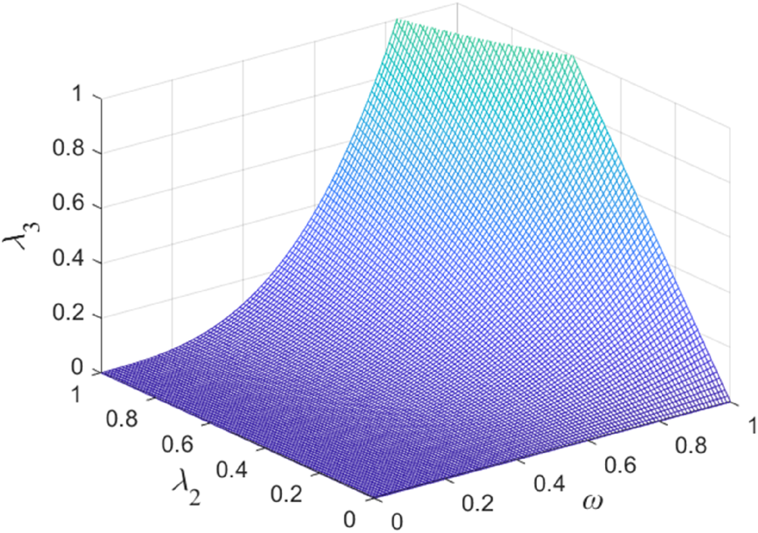

In Figure 4, the X-axis represents the natural frequency of the primary system, the Y-axis represents the nonlinear damping coefficient λ₂, and the Z-axis represents the cubic stiffness λ₃ coefficient. From the figure, it can be seen that when the parameters selected for the nonlinear damping NES system are located on and above the three-dimensional surface, the system is able to achieve target energy transfer, which satisfies the relationship in equation (6). When the natural frequency of the primary system is 1, with increasing nonlinear damping coefficient, the cubic stiffness coefficient increases monotonically, and the relationship between the two coefficients is a straight line with a slope of $\sqrt{3}$ . Therefore, when selecting the parameters, the ratio of λ₂ and λ₃ should be greater than or equal to $\sqrt{3}$ , so that the system can achieve TET. Using the coordinates of extreme points, the energy transfer efficiency equation of the nonlinear damping NES system is obtained

E_{t r} = 1 - \frac{E_{1 -}}{E_{1 +}} = 1 - \frac{(2 λ_{3} + h) ({λ_{3}}^{2} + 3 {λ_{2}}^{2} ω^{6} - λ_{3} h)}{(2 λ_{3} - h) ({λ_{3}}^{2} + 3 {λ_{2}}^{2} ω^{6} + λ_{3} h)}

(15)

Figure 5 shows the energy transfer efficiency curve of the nonlinear damping NES system, with cubic linear damping coefficient is drawn, and parameters are selected as λ₃ = 1.2, ω = 1.

Figure 5.

Relationship between nonlinear damping coefficient and energy transfer efficiency.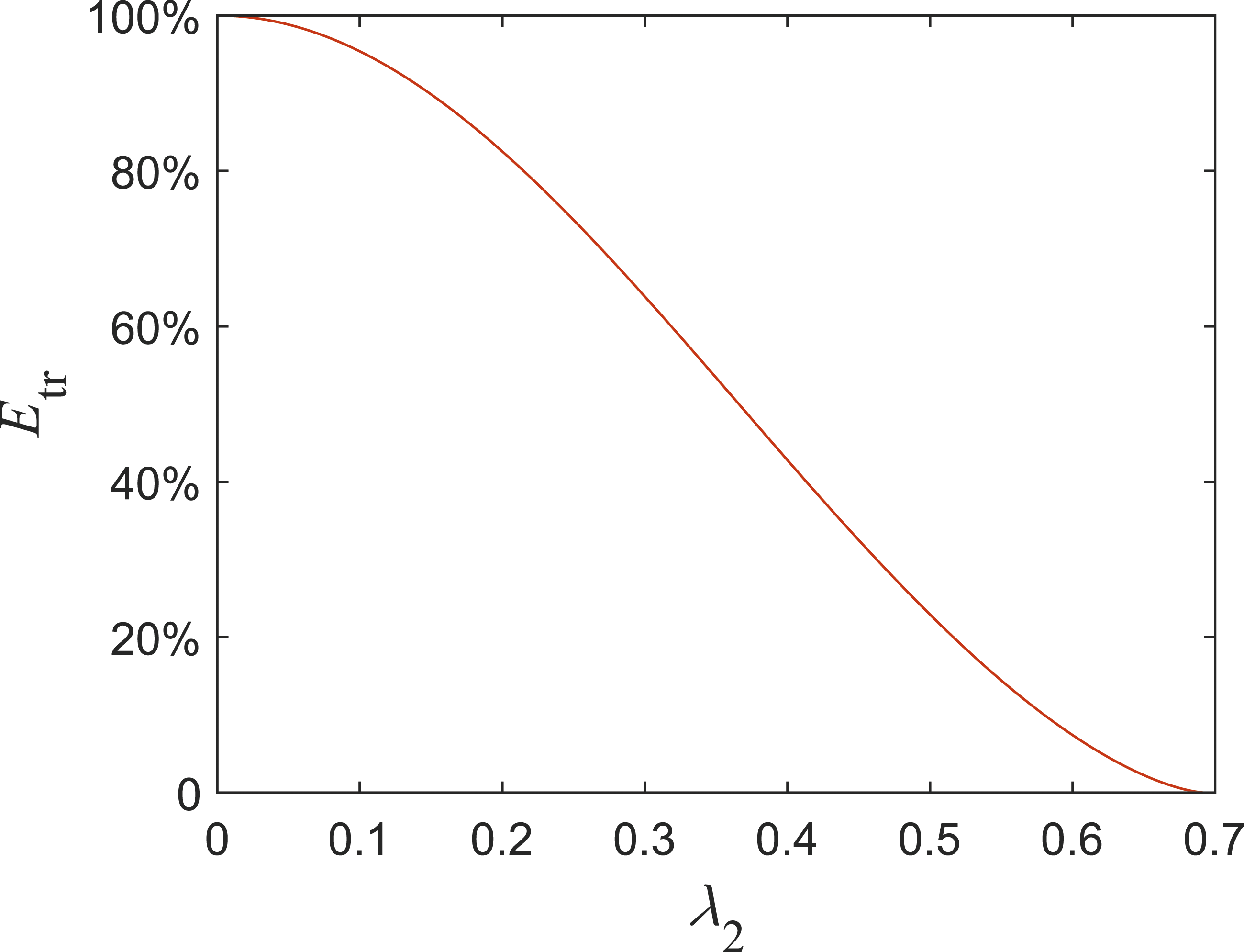

In Figure 5, the energy transfer efficiency of the nonlinear damping NES system gradually decreases with gradual increase of the nonlinear damping coefficient. When the nonlinear damping coefficient reaches the critical value, the energy transfer efficiency drops to 0, and the coordinate of the critical value is (0.691, 0). Therefore, in order to ensure the stability of the nonlinear damping NES system and other parameters are selected unchanged, the nonlinear damping coefficient should be selected as small as possible to ensure that the system has a high energy transfer efficiency.

The influence of the cubic stiffness coefficient and natural frequency on the energy transfer efficiency of the system are shown in Figure 6.

Figure 6.

The relationship between the system parameters of NES and energy transfer efficiency.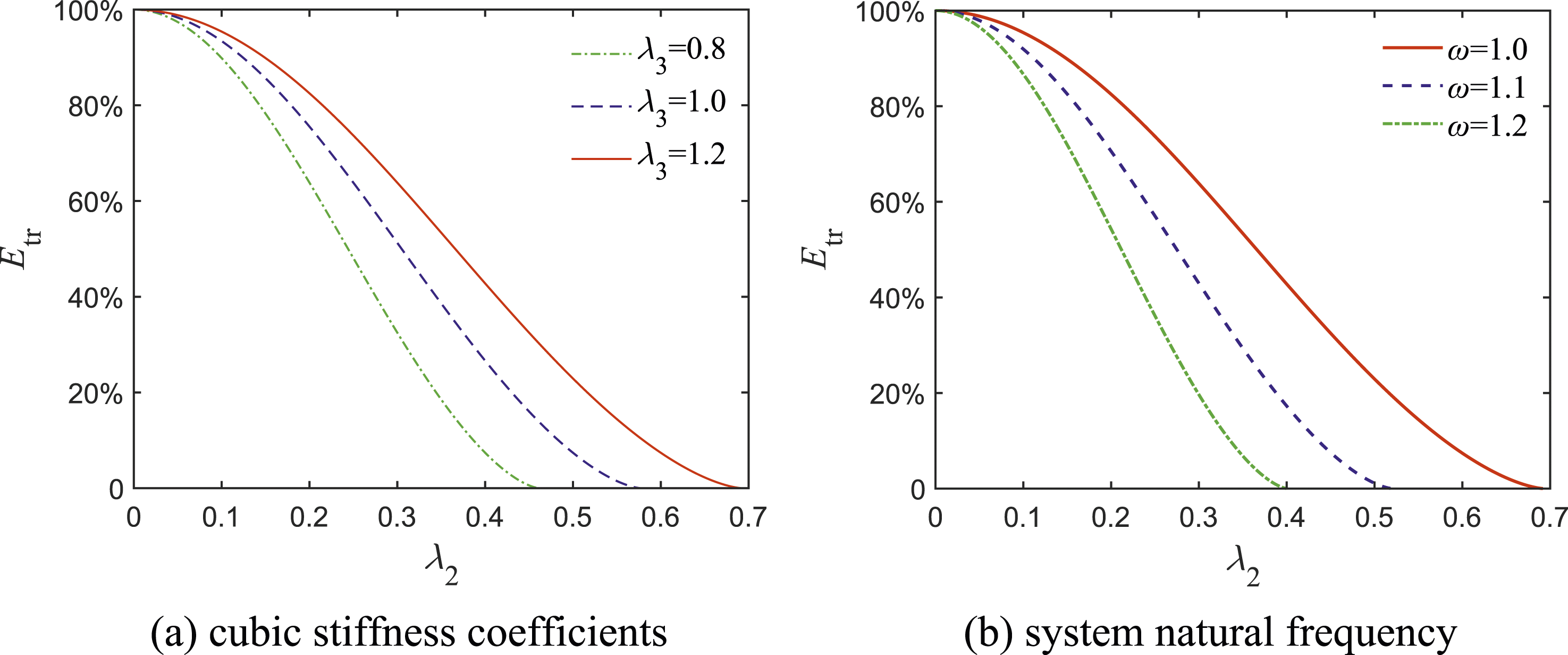

Figure 6(a) shows that, as the cubic stiffness coefficient increases, the energy transfer efficiency curve of the system with the nonlinear damping coefficient gradually shifts to the right. This indicates that, when the nonlinear damping coefficient remains constant, the energy transfer efficiency of the system is directly proportional to the cubic stiffness coefficient. The higher the cubic stiffness coefficient, the higher the energy transfer efficiency of the system. For the same reason, Figure 6(b) shows that the energy transfer efficiency of the system is inversely proportional to the natural frequency of the system. The greater the natural frequency of the system, the lower the energy transfer efficiency of the system. Therefore, a larger cubic stiffness coefficient and a smaller natural frequency should be selected for a higher energy transfer efficiency, with other parameters being held constant.

Analysis of saddle-node bifurcation

Boundary equation derivation

A type of static bifurcation in nonlinear dynamics, saddle-node bifurcation can be used to describe the emergence and disappearance of equilibrium points in a system. It can also be used to express the relationship between the number of equilibrium points and system parameters.

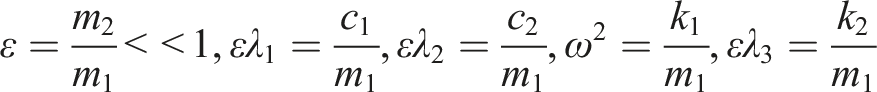
The parameters are introduced as follows

t = ω_{1} T, ω_{1} = \sqrt{\frac{k_{1}}{m_{1}}}, ε = \frac{m_{2}}{m_{1}} < < 1, ω = \frac{Ω}{ω_{1}}, w_{1} = \frac{x_{1}}{l}, w_{2} = \frac{x_{2}}{l} ε λ_{1} = \frac{c_{1}}{m_{1} ω_{1}}, ε λ_{2} = \frac{c_{2}}{m_{1} ω_{1}}, ε λ_{3} = \frac{k_{2}}{m_{1} {ω_{1}}^{2}}, ε f = \frac{F}{l k_{1}}

where l is the static shape variable of the primary system spring under the action of gravity. Then, equation (1) can be rewritten

{\begin{cases} {\ddot{w}}_{1} + ε λ_{1} {\dot{w}}_{1} + w_{1} + ε λ_{2} {({\dot{w}}_{1} - {\dot{w}}_{2})}^{3} + ε λ_{3} {(w_{1} - w_{2})}^{3} = ε f \cos (ω t) \\ ε {\ddot{w}}_{2} + ε λ_{2} {({\dot{w}}_{2} - {\dot{w}}_{1})}^{3} + ε λ_{3} {(w_{2} - w_{1})}^{3} = 0 \end{cases}

(16)

One assumption made in equation (16) should be emphasized here. As a matter of 1:1 resonance condition, assume that the external excitation frequency is close to the natural frequency of the system, defining ω = 1+εσ, where σ represents the frequency detuning parameter.^25,26 Using a change of state variables, $u = w_{1} + ε w_{2}$ , $v = w_{1} - w_{2}$ , equation (16) can be reduced to

{\begin{cases} \ddot{u} + \frac{u + ε v}{1 + ε} = ε f \cos [(1 + ε σ) t] \\ \ddot{v} + (1 + ε) λ_{2} {\dot{v}}^{3} + (1 + ε) λ_{3} v^{3} + \frac{u + ε v}{1 + ε} = ε f \cos [(1 + ε σ) t] \end{cases}

(17)

Then introducing complex variables

ϕ_{1} e^{i (1 + ε σ)} = \dot{u} + i u

ϕ_{2} e^{i (1 + ε σ)} = \dot{v} + i v

, equation (17) can be rewritten

{\begin{cases} {\dot{ϕ}}_{1} + i ε σ ϕ_{1} + \frac{i ε (ϕ_{1} - ϕ_{2})}{2 (1 + ε)} = \frac{ε f}{2} \\ {\dot{ϕ}}_{2} + i ε σ ϕ_{2} + \frac{i (ϕ_{2} - ϕ_{1})}{2 (1 + ε)} + \frac{3 (1 + ε) ϕ_{2} {| ϕ_{2} |}^{2}}{8} (λ_{2} - i λ_{3}) = \frac{ε f}{2} \end{cases}

(18)

In order to study the equilibrium state of the system, let the derivative term in the above equations be zero; then, the equilibrium state equation of the system is given by

{\begin{cases} i ε σ ϕ_{10} + \frac{i ε}{2 (1 + ε)} (ϕ_{10} - ϕ_{20}) = \frac{ε f}{2} \\ i ε σ ϕ_{20} + \frac{i}{2 (1 + ε)} (ϕ_{20} - ϕ_{10}) + \frac{3 (1 + ε) ϕ_{20} {| ϕ_{20} |}^{2}}{8} (λ_{2} - i λ_{3}) = \frac{ε f}{2} \end{cases}

(19)

where

ϕ_{10}

and

ϕ_{20}

are equilibrium points of the system. The solution to equation (19) is

{\begin{cases} ϕ_{10} = \frac{ϕ_{20} - i (1 + ε) f}{2 ε σ + 2 σ + 1} \\ \frac{9 {λ_{2}}^{2} + 9 {λ_{3}}^{2}}{16} {| ϕ_{20} |}^{6} - 3 λ_{3} M σ {| ϕ_{20} |}^{4} + 4 M^{2} σ^{2} {| ϕ_{20} |}^{2} = M^{2} f^{2} \end{cases}

(20)

where M = (2εσ+1)/(2εσ+2σ+1); the second equation in equation (20) can be expressed as

α_{1} Z + α_{2} Z^{2} + α_{3} Z^{3} = f^{2}

(21)

where

Z = {| ϕ_{20} |}^{2}

α_{1} = 4 σ^{2}

α_{2} = - 3 λ_{3} σ / M

, and

α_{3} = (9 λ_{2}^{2} + 9 λ_{3}^{2}) / 16 M^{2}

. Taking the derivative of equation (21) with respect to Z yields

α_{1} + 2 α_{2} Z + 3 α_{3} Z^{2} = 0

(22)

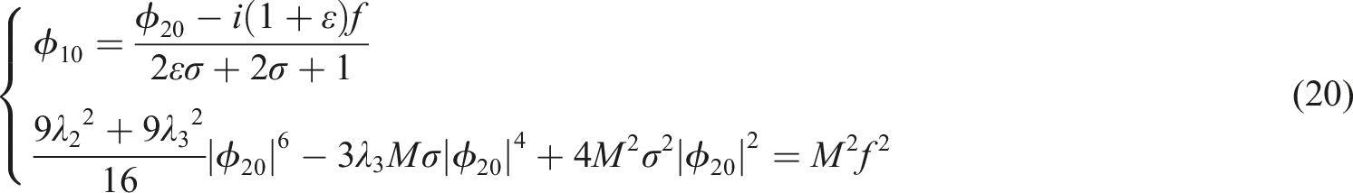
By combining Eq. (21) and Eq. (22), the saddle-node bifurcation boundary equation of the system is given by

\frac{10 {α_{2}}^{3} - 27 α_{1} α_{2} α_{3} \pm 10 {α_{2}}^{2} \sqrt{{α_{2}}^{2} - 3 α_{1} α_{3}} + 3 α_{1} (\mp 4 α_{3} \sqrt{{α_{2}}^{2} - 3 α_{1} α_{3}} + 9 α_{1} f^{2})}{27 {α_{3}}^{2}} = 0

(23)

Saddle-node bifurcation diagram of the system

Equation (23) shows the relationship between the external excitation amplitude and the other parameters. Equation (23) is not only used to represent the saddle-node bifurcation boundary curve, but also to analyze periodic solutions.

The parameters are selected as ε = 0.05, λ₃ = 1.2, σ = 0.5, as shown in Figure 7.

Figure 7.

Saddle-node bifurcation diagram of nonlinear damping NES system.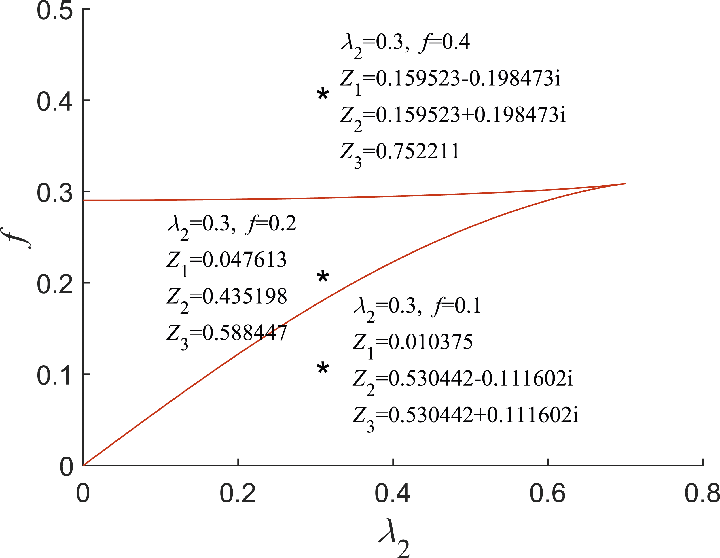

Figure 7 shows that the saddle-node bifurcation boundary curve of the nonlinear damping NES system is roughly triangular. Moreover, the saddle-node bifurcation diagram is divided into two parts by the boundary curve. Taking three points on diagram to study the equilibrium point of the system, taking points inside the triangle formed by the coordinate axis and the boundary curve, for λ₂ = 0.3, f = 0.2, which can get three different real roots, representing the system has three equilibrium points. Then, taking points outside, whether on the upper part of the diagram or on the lower part, produces only a real root, meaning that the system has only one equilibrium point. For example, for λ₂ = 0.3, f = 0.4 or λ₂ = 0.3, f = 0.1, there is only one real solution. Therefore, when the nonlinear damping coefficient is constant, different numbers of equilibrium points can be obtained by changing the external excitation amplitude.

Selecting the same parameters to draw the comparison of saddle-node bifurcation boundary curves of linear damping NES system and nonlinear damping NES system, as shown in Figure 8.

Figure 8.

Comparison of saddle-node bifurcation between linear damping and nonlinear damping systems.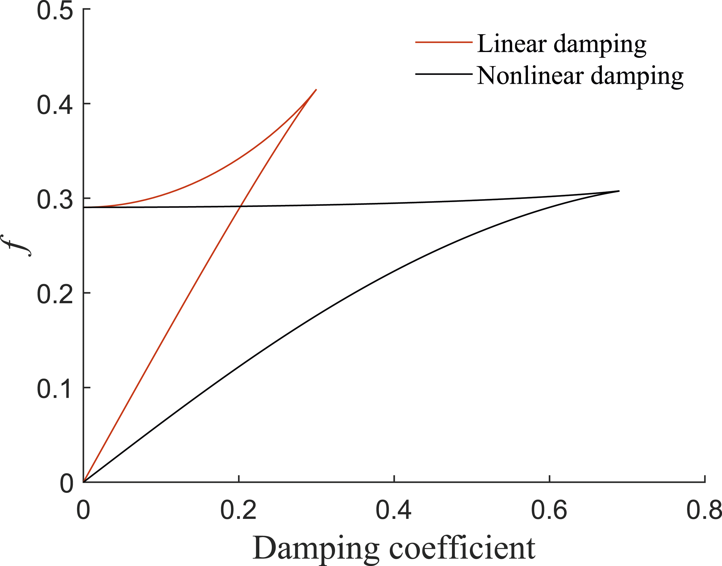

Figure 8 shows that, when other parameters are the same, the saddle-node bifurcation area of the nonlinear damping NES system is larger than that of the linear damping NES system. This indicates that the area of the nonlinear damping NES system obtains three equilibrium points is larger than the linear damping NES system. Saddle-node bifurcation is more likely to occur in nonlinear damping NES system than in linear damping NES system.

The influence of the mass ratio, cubic stiffness coefficient, and frequency detuning parameter on the saddle-node bifurcation diagram is now studied. For ε as 0.05, 0.1, 0.15, and 0.2, respectively, as shown in Figure 9.

Figure 9.

Saddle-node bifurcation diagram for different mass ratios.

Figure 9 shows that, with increasing mass ratio, the external excitation amplitude of the coordinate increases, while the nonlinear damping coefficient remains constant. Moreover, the triangular area formed by the axis and the saddle-node bifurcation boundary curve increases. This means that the region from which the three equilibrium points of the system can be obtained increases.

When the other parameters are held constant, the following cubic stiffness coefficients are used: 0.9, 1.2, 1.5, and 1.8, as shown in Figure 10.

Figure 10.

Saddle-node bifurcation diagram for different cubic stiffness coefficients.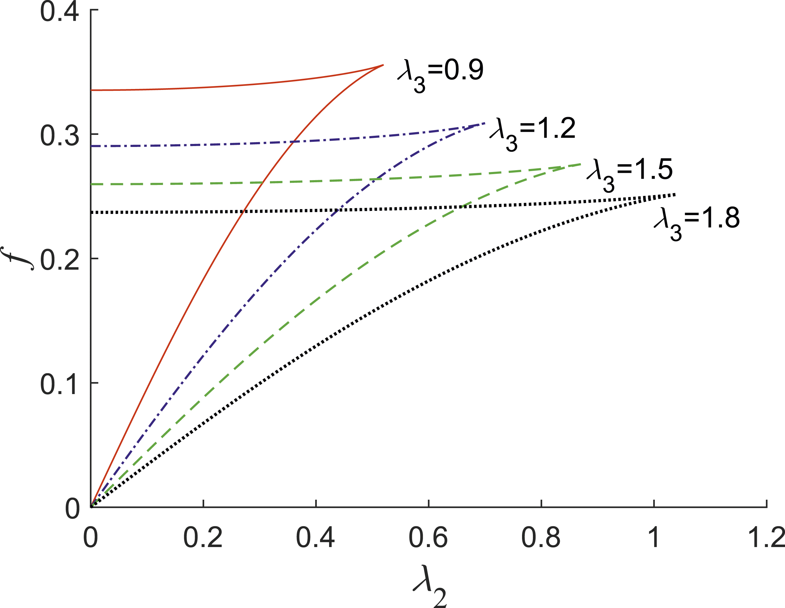

Figure 10 shows that, with increasing cubic stiffness coefficient. Although the external excitation amplitude of the ordinate is gradually decreasing, the triangular area formed by the saddle-node bifurcation boundary curve and coordinate axis is constantly increasing. This indicates that the region from which the three equilibrium points can be obtained increases. Without affecting the other parameters of the system, a smaller mass ratio and a larger cubic stiffness coefficient are chosen as far as possible to ensure that the system has a larger area for obtaining the number of equilibrium points.

The influence of frequency detuning is now studied, as shown in Figure 11.

Figure 11.

Saddle-node bifurcation diagram for different frequency detuning parameters.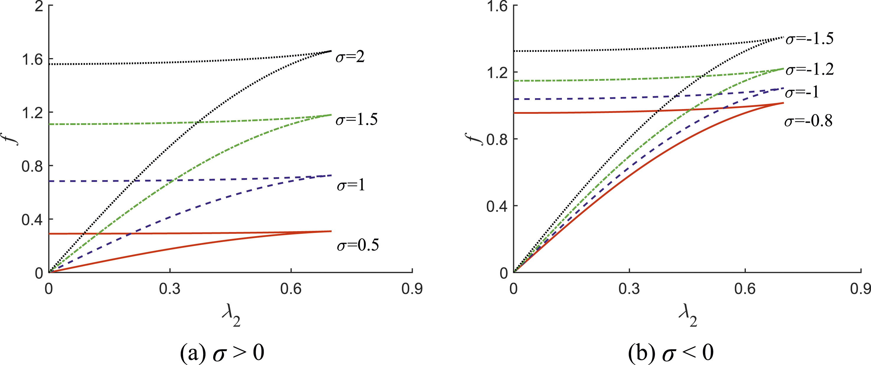

According to the equation: $ω = 1 + ε σ$ . Figure 11(a) shows that the external excitation frequency is greater than the natural frequency of the primary system. Figure 11(b) shows that the external excitation frequency is less than the natural frequency of the primary system. When $σ > 0$ , the area of the triangle increases with increasing frequency detuning, and the external excitation amplitude interval with the three equilibrium points also increases. In contrast, when $σ < 0$ , the smaller the frequency detuning parameter, the larger the area of the triangle. It should be noted in particular that, no matter how the frequency detuning parameter changes, the nonlinear damping coefficient of the abscissa coordinate remains unchanged. Only the external excitation amplitude changes with the change. Changing the frequency detuning parameter and changing the mass ratio have similar effects on the saddle-node bifurcation.

SMR analysis of nonlinear damping NES system

Slow invariant manifold analysis under SMR

The slow invariant manifold is the response surface of the system that contains only the slow variable parameters, and according to equation (18), the system is a four-dimensional phase space. The slow variable flow consists of four variables: for $ϕ_{2}$ , ${\dot{ϕ}}_{2}$ , they are fast variables; and for $ϕ_{1}$ , ${\dot{ϕ}}_{1}$ , they are slow variables. In order to facilitate the subsequent calculation, reducing the number of variables in the phase plane of the equation. The reduced equations for this system are obtained as follows

{\ddot{ϕ}}_{2} + \frac{d}{d t} [\frac{i (1 + 4 ε σ)}{2} ϕ_{2} + \frac{3 (1 + ε)}{8} (λ_{2} - i λ_{3}) {| ϕ_{2} |}^{2} ϕ_{2}] + ϕ_{2} - \frac{ε σ}{2} (1 + 2 ε σ) + \frac{3 i ε (1 + 2 σ + 2 ε σ)}{16} (λ_{2} - i λ_{3}) {| ϕ_{2} |}^{2} - \frac{i ε f}{4} (1 + 2 ε σ) = 0

(24)

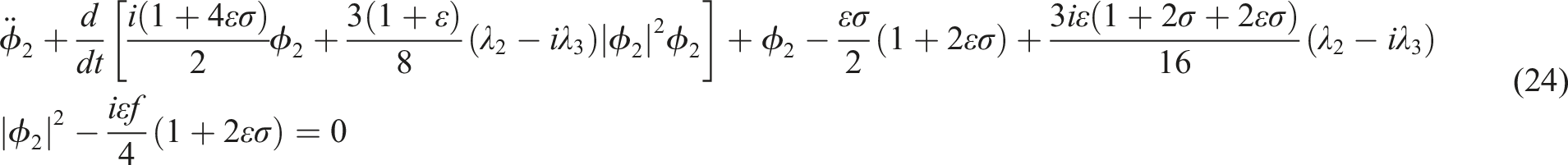
The solution is the same as before, by introducing the timescale. The equation (24) can be rewritten

{\begin{cases} ε^{0} : {D_{0}}^{2} ϕ_{2} + \frac{i D_{0} ϕ_{2}}{2} + \frac{3 D_{0} ϕ_{2}}{8} (λ_{2} {| ϕ_{2} |}^{2} - i λ_{3} {| ϕ_{2} |}^{2}) = 0 \\ \begin{array}{l} ε^{1} : 2 D_{0} D_{1} ϕ_{2} + \frac{D_{0} ϕ_{2}}{8} (16 i σ + 3 λ_{2} {| ϕ_{2} |}^{2} - 3 i λ_{3} {| ϕ_{2} |}^{2}) + \frac{D_{1} ϕ_{2}}{8} (4 i + 3 λ_{2} {| ϕ_{2} |}^{2} \\ - 3 i λ_{3} {| ϕ_{2} |}^{2}) - \frac{σ}{2} ϕ_{2} + \frac{3 i (1 + 2 σ) ϕ_{2}}{16} (λ_{2} {| ϕ_{2} |}^{2} - i λ_{3} {| ϕ_{2} |}^{2}) - \frac{i f}{4} = 0 \end{array} \end{cases}

(25)

Study $ϕ_{2}$ about the approximate solution of the fast varying timescale, integrating the first equation in the equation (25) can obtain

D_{0} ϕ_{2} + \frac{i ϕ_{2}}{2} + \frac{3 ϕ_{2}}{8} (λ_{2} {| ϕ_{2} |}^{2} - i λ_{3} {| ϕ_{2} |}^{2}) = Q (t_{1})

(26)

where Q is an arbitrary function on a slow varying timescale. Let

D_{0} ϕ_{2} = 0

, which can get the equilibrium equation of the system only with respect to variable

t_{1}

. Then, equation (26) is rewritten

\frac{i ϕ_{2}}{2} + \frac{3 ϕ_{2}}{8} (λ_{2} {| ϕ_{2} |}^{2} - i λ_{3} {| ϕ_{2} |}^{2}) = Q (t_{1})

(27)

Using the magnitude and phase angle to represent complex variables,

ϕ_{2} (t_{1}) = N (t_{1}) e^{j θ (t_{1})}

, equation (27) can be reduced to

\frac{9}{16} ({λ_{2}}^{2} + {λ_{3}}^{2}) N^{6} - \frac{3}{2} λ_{3} N^{4} + {N_{d}}^{2} = 4 {| Q |}^{2}

(28)

Equation (28) is the slow invariant manifold equation of the system. The selected parameters are λ₂ = 0.2, λ₃ = 1.2; and the slow invariant manifold diagram is shown in Figure 12.

Figure 12.

Slow invariant manifold of the system under periodic excitation.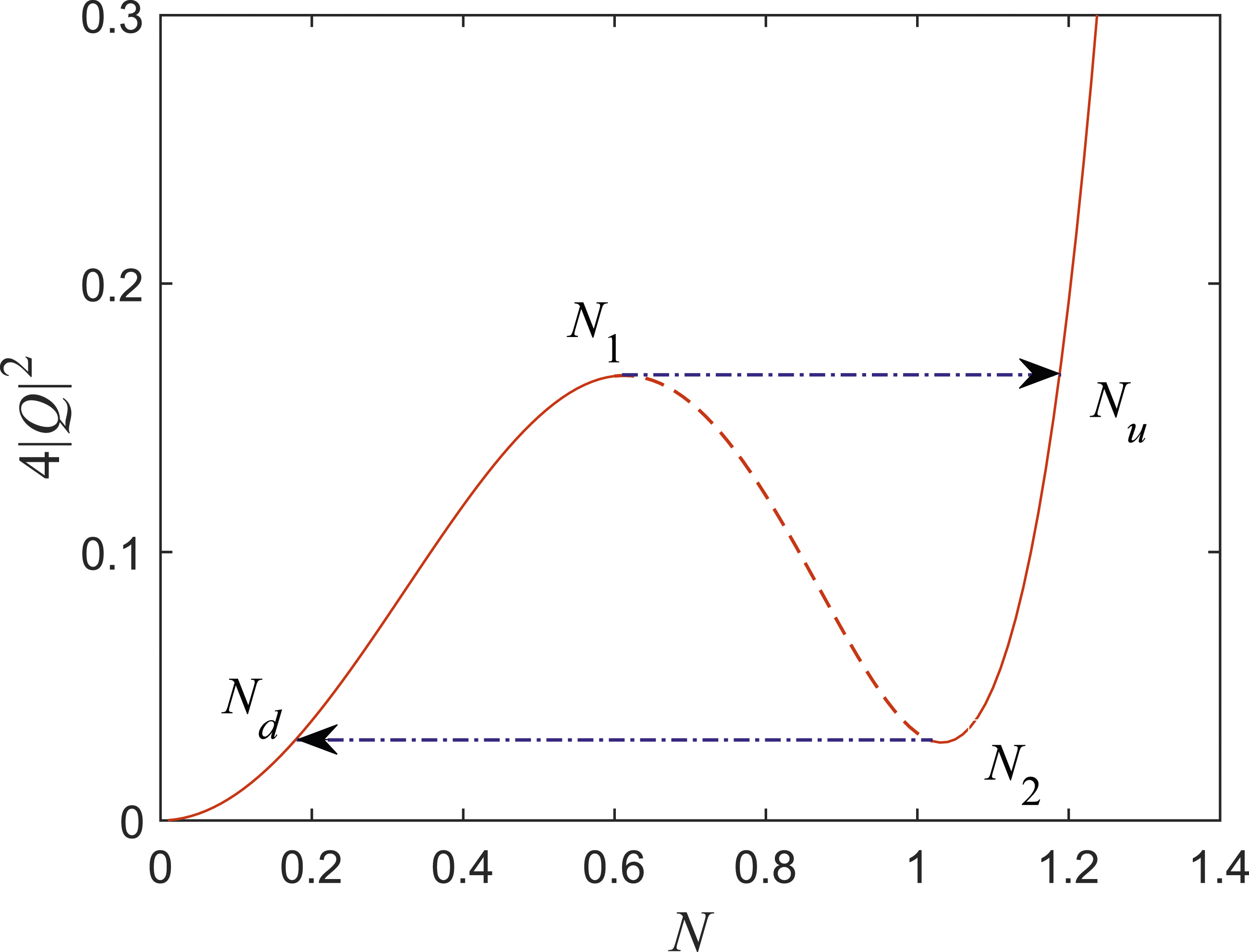

In Figure 12, the real line represents the stable part of the system, the broken line represents the unstable part, and the chain line with arrows represents the jump trajectory of the slow amplitude of the system. The slow amplitude N of the system moves along the curve of the slow invariant manifold diagram. When moving along the left stable part meets a point N₁, the system does not move along the middle manifold, because the manifold is unstable. Therefore, the system jumps from N₁ to N_u and continues to move along the stable part on the right. When it meets point N₂, it jumps from point N₂ to N_d and continues to move along the stable part on the left. Form a continuous jumping loop, which the slow amplitude of the system presents a periodic change, this periodic change is called SMR. When the ratio of the external excitation frequency to the natural frequency of the system is 1:1, there is a quasi-periodic response in the nonlinear damping NES system. The variation of the slow-change amplitude is periodic, which enables the NES to provide excellent vibration suppression for the primary system.

Analysis of the necessary conditions for SMR generation

Setting Z = N², equation (28) can be rewritten as

\frac{9}{16} ({λ_{2}}^{2} + {λ_{3}}^{2}) Z^{3} - \frac{3}{2} λ_{3} Z^{2} + Z = 4 {| Q |}^{2}

(29)

The derivation of the above equation is expressed as

\frac{27}{16} ({λ_{2}}^{2} + {λ_{3}}^{2}) Z^{2} - 3 λ_{3} Z + 1 = 0

(30)

The solution of the equation is

Z_{1, 2} = \frac{8 λ_{3} \mp \sqrt{{λ_{3}}^{2} - 3 {λ_{2}}^{2}})}{9 ({λ_{2}}^{2} + {λ_{3}}^{2})} \Rightarrow N_{1, 2} = \sqrt{\frac{8 λ_{3} \mp \sqrt{{λ_{3}}^{2} - 3 {λ_{2}}^{2}})}{9 ({λ_{2}}^{2} + {λ_{3}}^{2})}}

(31)

Since the slow invariant manifold of the system at the jump point corresponds to a constant value, according to equation (28), the resulting expression is

\frac{9}{16} ({λ_{2}}^{2} + {λ_{3}}^{2}) {Z_{1, 2}}^{3} - \frac{3}{2} λ_{3} {Z_{1, 2}}^{2} + Z_{1, 2} = \frac{9}{16} ({λ_{2}}^{2} + {λ_{3}}^{2}) {Z_{u, d}}^{3} - \frac{3}{2} λ_{3} {Z_{u, d}}^{2} + Z_{u, d}

(32)

The solution of equation (32) is

Z_{u, d} = \frac{8 λ_{3} \pm 8 \sqrt{{λ_{3}}^{2} - 3 {λ_{2}}^{2}})}{9 ({λ_{2}}^{2} + {λ_{3}}^{2})} \Rightarrow N_{u, d} = \sqrt{\frac{8 λ_{3} \pm 8 \sqrt{{λ_{3}}^{2} - 3 {λ_{2}}^{2}})}{9 ({λ_{2}}^{2} + {λ_{3}}^{2})}}

(33)

Considering the timescale ε¹, when $t_{0} \to \infty$ , the second equation in equation (25) can be rewritten

\frac{\partial ϕ_{2}}{\partial t_{1}} [\frac{i}{2} + \frac{3}{4} (λ_{2} {| ϕ_{2} |}^{2} - i λ_{3} {| ϕ_{2} |}^{2})] + \frac{3 {ϕ_{2}}^{2} (λ_{2} - i λ_{3})}{8} \frac{\partial {\bar{ϕ}}_{2}}{\partial t_{1}} = C

(34)

where

C = \frac{i f}{4} + \frac{σ}{2} ϕ_{2} - \frac{3 i (1 + 2 σ) ϕ_{2} {| ϕ_{2} |}^{2}}{16} (λ_{2} - i λ_{3})

(35)

Using complex variables $ϕ_{2} (t_{1}) = N (t_{1}) e^{j θ (t_{1})}$ , we can obtain

{\begin{cases} G (N) \frac{\partial N}{\partial t_{1}} = - \frac{3 λ_{2}}{4} N^{3} + \frac{3 f}{4} N^{2} (λ_{2} \sin θ - λ_{3} \cos θ) + f \cos θ \\ \begin{array}{l} G (N) \frac{\partial θ}{\partial t_{1}} = \frac{9 f}{4} N (λ_{2} \cos θ + λ_{3} \sin θ) + \frac{3 λ_{3}}{4} (1 + 8 σ) N^{2} - \frac{f}{N} \\ - \frac{27 (1 + 2 σ)}{16} ({λ_{2}}^{2} + {λ_{3}}^{2}) N^{4} - 2 σ \end{array} \end{cases}

(36)

where

G (N) = 2 [\frac{27}{16} ({λ_{2}}^{2} + {λ_{3}}^{2}) N^{4} - 3 λ_{3} N^{2} + 1]

(37)

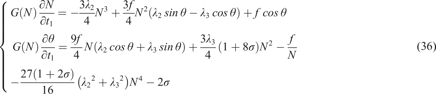
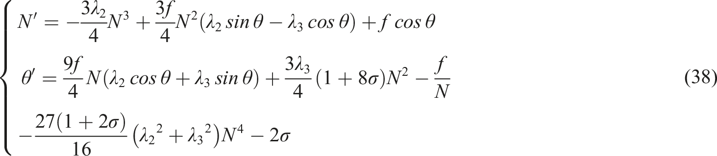
According to the analysis of slow invariant manifolds, when G(N) = 0, jumping occurs. In order to avoid creating singularities, rescaling equation (36) to the time scale, and the equation can be transformed into

{\begin{cases} N^{'} = - \frac{3 λ_{2}}{4} N^{3} + \frac{3 f}{4} N^{2} (λ_{2} \sin θ - λ_{3} \cos θ) + f \cos θ \\ \begin{array}{l} θ^{'} = \frac{9 f}{4} N (λ_{2} \cos θ + λ_{3} \sin θ) + \frac{3 λ_{3}}{4} (1 + 8 σ) N^{2} - \frac{f}{N} \\ - \frac{27 (1 + 2 σ)}{16} ({λ_{2}}^{2} + {λ_{3}}^{2}) N^{4} - 2 σ \end{array} \end{cases}

(38)

The selected parameters are λ₂ = 0.2, λ₃ = 1.2, f = 3. The above equation is used to obtain the phase trajectories for different frequency detuning parameters, as shown in Figure 13.

Figure 13.

System phase trajectory diagram of frequency detuning parameter changes.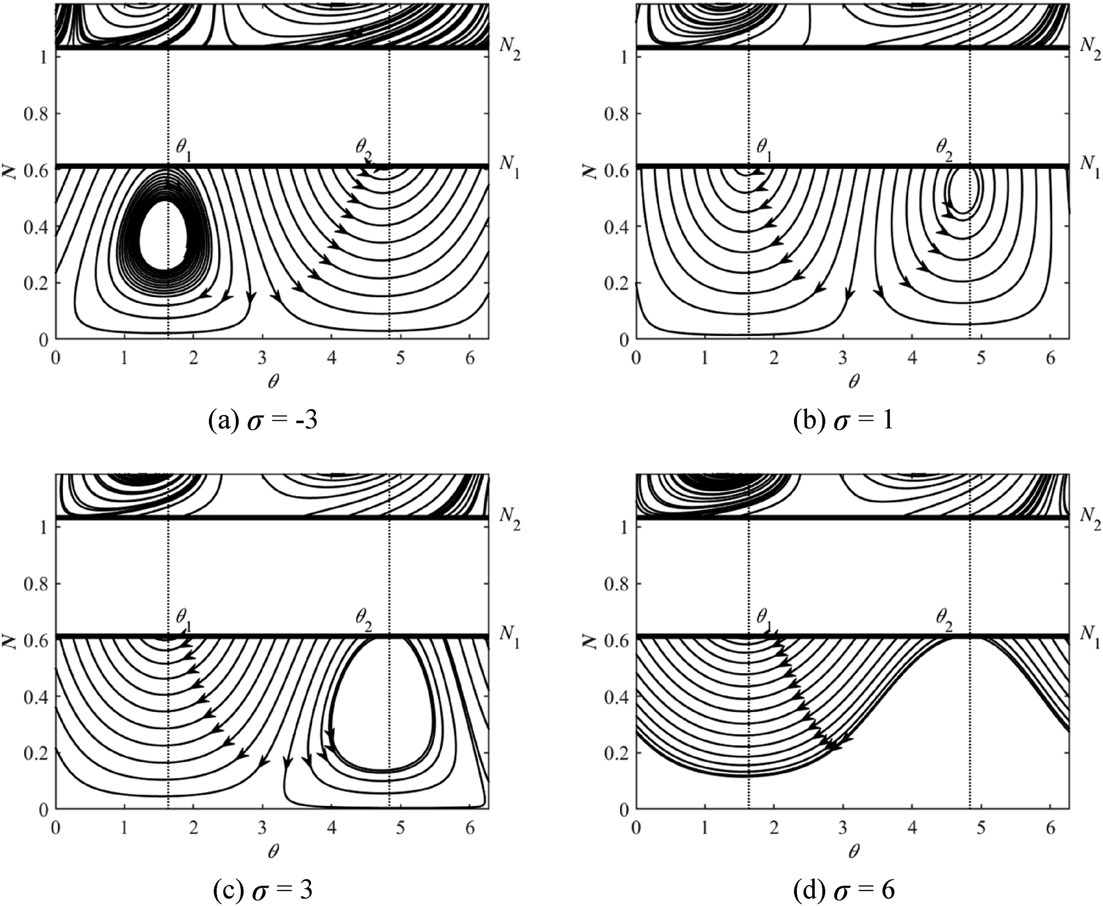

In Figure 13, θ₁ and θ₂ are the initial phase angles of the system. The arrow represents the direction of the phase trajectory. The stable part of the slow invariant manifold is reflected below the horizontal line at N₁ and above the horizontal line at N₂, and the two horizontal lines in the phase trajectory diagram represent the return line in the slow invariant manifold diagram. Only when the phase trajectory that starts from the horizontal line returns to the horizontal line, is it possible to jump in the unstable part and reach the other stable branch part. Only in this way can the system be guaranteed to produce SMR.

In Figure 13(a), all phase trajectories on the right side of the horizontal line N₁ can start from the initial phase angle interval [θ₁, θ₂], then move down, and return to the horizontal line N₁, which jumps to the horizontal line N₂ and reaches the stable branch above. However, the phase trajectories on the left side cannot all return to the horizontal line, because an attractor appears on the left side, around which parts of the phase trajectories converge. By adjusting the frequency detuning parameter, the attractor gradually disappears; the phase trajectory at this time is shown in Figure 13(b). All phase trajectories under the horizontal line N₁ return before jumping to the horizontal line N₂. With gradual increase in the frequency detuning parameter, the phase trajectory to the right of the horizontal line N₁ disappears, resulting in no jump near the initial phase angle of the system. The phase trajectory jumps from the horizontal line N₁ to the horizontal line N₂ and then back to the horizontal line N₁. During this process, the response amplitude of the system changes constantly, which makes it possible for the system to realize SMR. Since the jumps occur in this interval, the initial phase angle interval [θ₁, θ₂] is also called the jump interval, and there is uncertainty in the jump process occurring in this interval. Therefore, it is necessary to use one-dimensional mapping to determine the interval of frequency detuning parameter in the existence of SMR.

According to equation (27), the initial phase angle relationship is given by

\arg Q = θ + \tan^{- 1} (\frac{4 - 3 λ_{3} Z}{3 λ_{2} Z})

(39)

Using Eqs. (30) and Eq. (39), setting T_i = (4-3λ₃Z_i)/3λ₂Z_i, i = 1,2,u,d, and the relationship between N_u and N_d phase angle is given by

θ_{u, d} = θ_{1, 2} + \tan^{- 1} (\frac{T_{1, 2} - T_{u, d}}{1 + T_{1, 2} T_{u, d}})

(40)

The selected parameters are λ₂ = 0.2, λ₃ = 1.2, f = 3. One-dimensional mapping of the system with different frequency detuning parameters is shown in Figure 14.

Figure 14.

One-dimensional map of frequency detuning variation.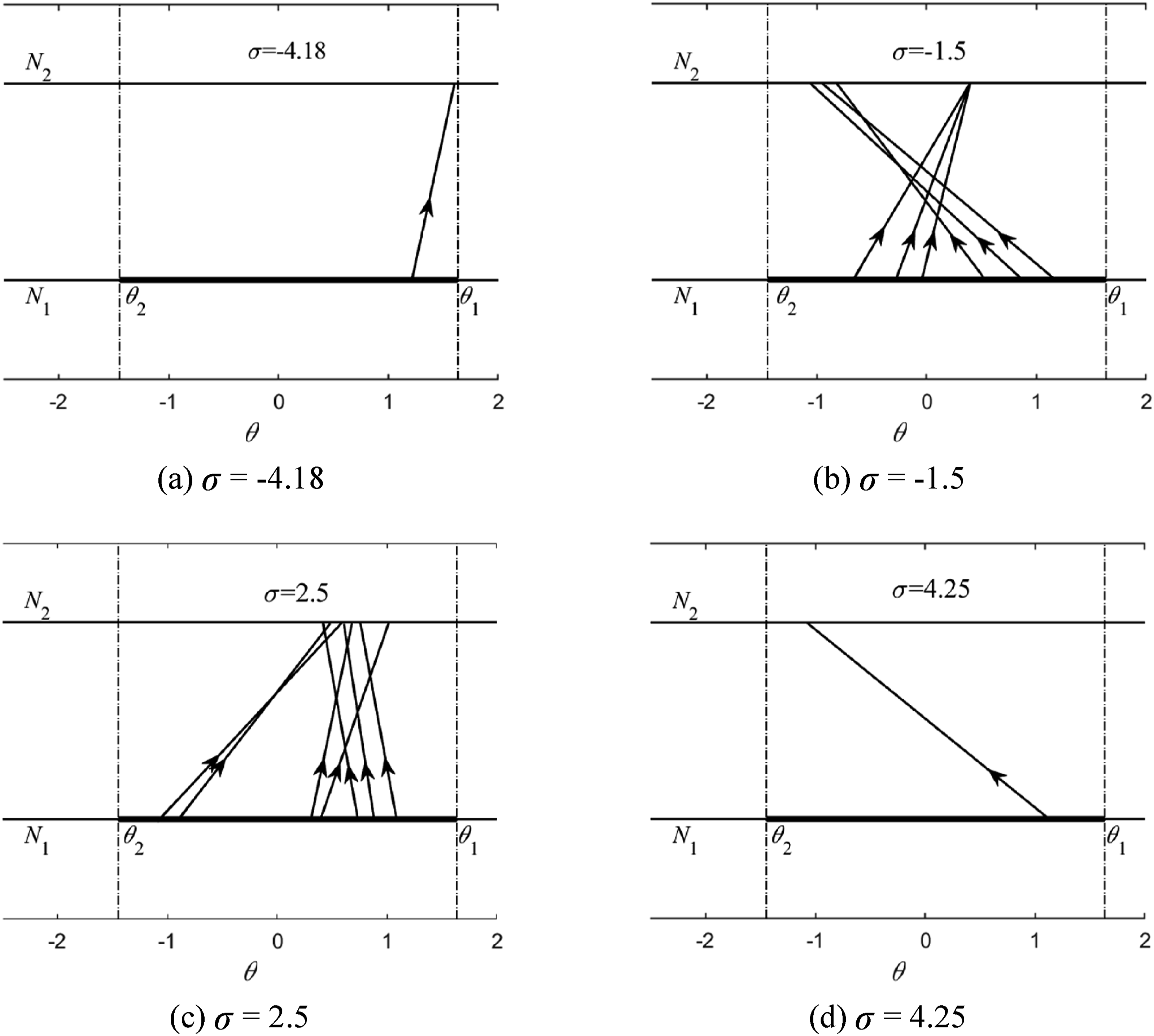

In Figure 14, the straight line with arrow represents the jump trajectory in the jump interval, called a one-dimensional mapping trajectory. In this paper, the frequency detuning parameter interval existing in the SMR is determined by changing the frequency detuning parameter. When the external excitation amplitude is equal to 3, the interval in which the SMR exists is [−4.18, 4.25]. Using the one-dimensional mapping diagram, the necessary conditions for the existence of SMR in nonlinear damping NES systems are determined.

Then, the influence of external excitation amplitude, nonlinear damping coefficient and cubic stiffness coefficient on the interval σ of the SMR is studied, respectively. Firstly, the influence of the external excitation amplitude is studied. By analyzing the one-dimensional mapping diagram when the external excitation amplitude is 3, 5, and 7, respectively, the interval σ in which the SMR exists when the external excitation amplitude changes is determined, as shown in Table 1.

Table 1.

The σ interval.

External excitation amplitude	σ Interval
f = 3	σ∈[−4.18, 4.25]
f = 5	σ∈[−7.12, 6.98]
f = 7	σ∈[−10.05, 9.66]

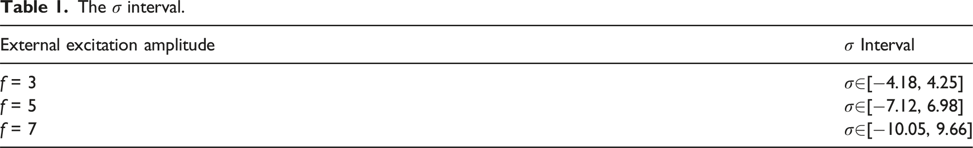
Table 1 shows that the interval length of the frequency detuning parameter is in a positive proportional relationship with the external excitation amplitude. This relationship can be approximated by the linear function y = 2.82x−0.02. The initial points of the interval σ in which SMR exists are inversely proportional to the external excitation amplitude. This relationship is approximated by the linear function y = −1.468x−0.22. The end points of the interval σ in which SMR exists are approximated by the linear function y = 1.353x+0.201. The functional relationship between the length of the frequency detuning parameter interval, the initial points of the interval σ where SMR exists, the end points of the interval σ where SMR exists, and the external excitation amplitude is shown in Figure 15.

Figure 15.

Diagram of the relationship between different external excitation amplitudes and σ intervals.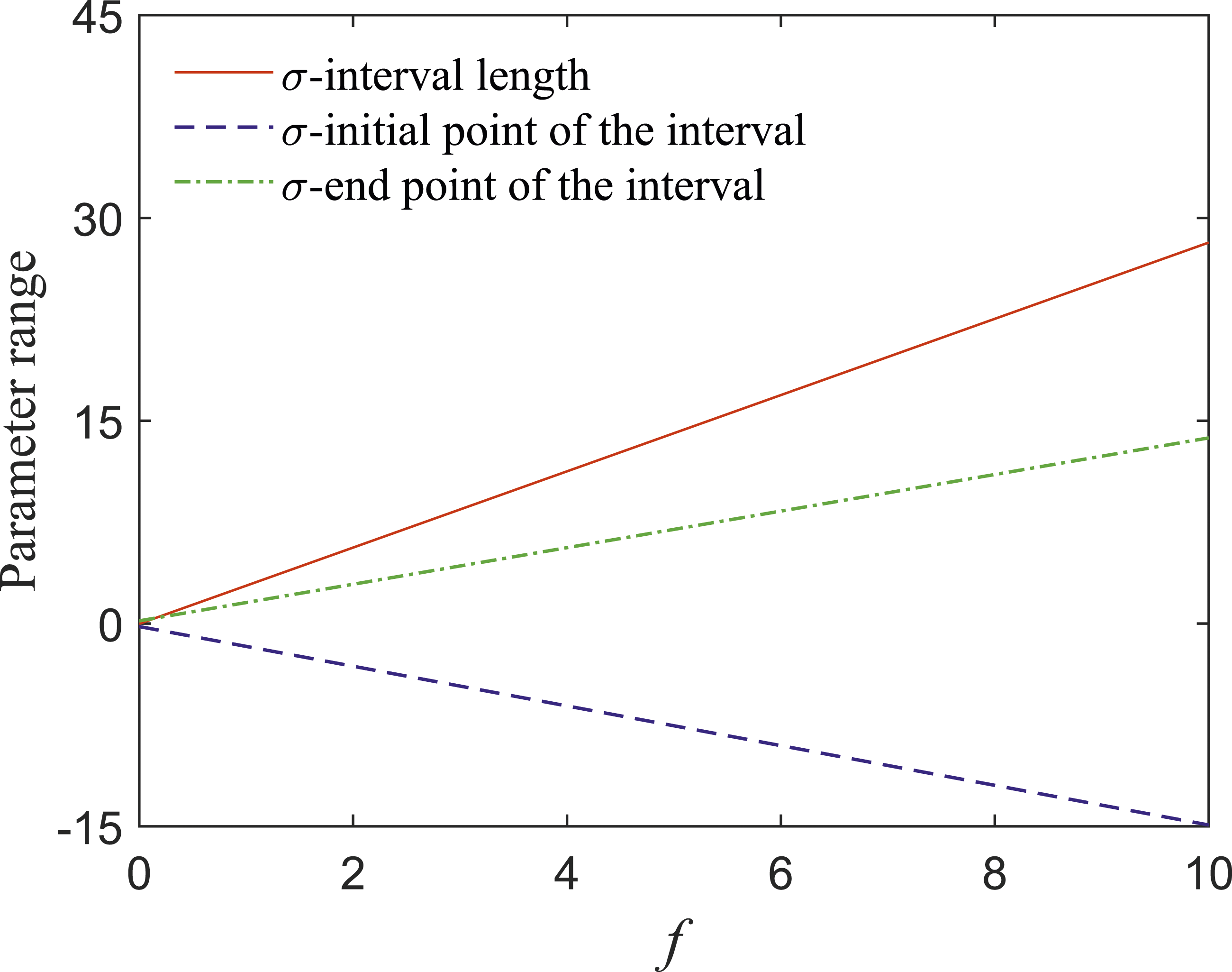

Table 1 and Figure 15 show that, to ensure system stability, as large an excitation amplitude as possible should be selected to increase the interval σ length of the frequency detuning parameter when the SMR exists. This maximizes the chance of the SMR in the nonlinear damping NES system.

Then, the influence of nonlinear damping coefficient on the interval σ existing in SMR is studied. By drawing one-dimensional mapping diagram with λ₂ of 0.2, 0.4, and 0.6, respectively, the interval σ existing in the strongly modulated response when the nonlinear damping coefficient changes is determined, as shown in Table 2.

Table 2.

The σ interval.

Nonlinear damping coefficient	σ Interval
λ₂ = 0.2	σ∈[−4.18, 4.25]
λ₂ = 0.4	σ∈[−3.89, 4.04]
λ₂ = 0.6	σ∈[−3.35, 3.61]

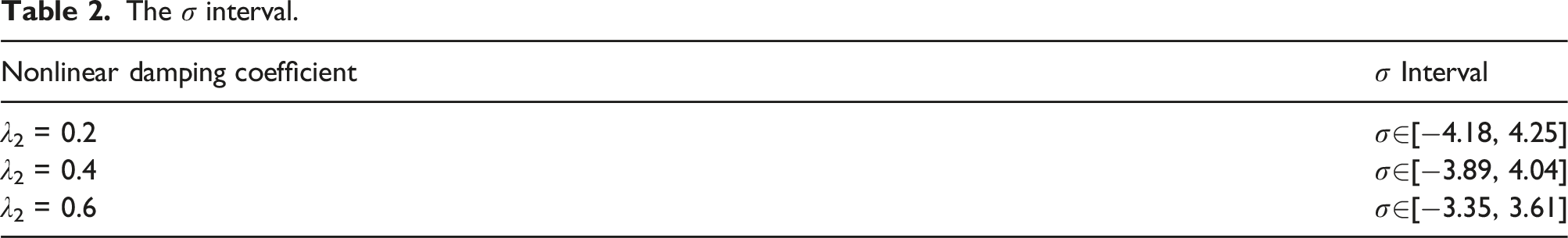
Table 2 shows that the length of the frequency detuning interval decreases with increasing nonlinear damping coefficient. The relationship between the two can be approximated by the quadratic function y = −5.125x²+0.425x+8.55. The initial points of the frequency detuning parameter interval σ of the SMR increase with increasing nonlinear damping coefficient. Moreover, the relationship between the two is given by y = 3.125x²−0.425x−4.22. The relationship between the end points of the interval σ where the SMR exists and the nonlinear damping coefficient is opposite to the initial coordinates and is approximated by the quadratic function y = −1.875x²−0.075x+4.34. The functional relationship between the length of the frequency detuning parameter interval, the initial points of the interval σ where the SMR exists, the end points of the interval σ where the SMR exists, and the nonlinear damping coefficient is shown in Figure 16.

Figure 16.

Diagram of different nonlinear damping coefficients and σ intervals.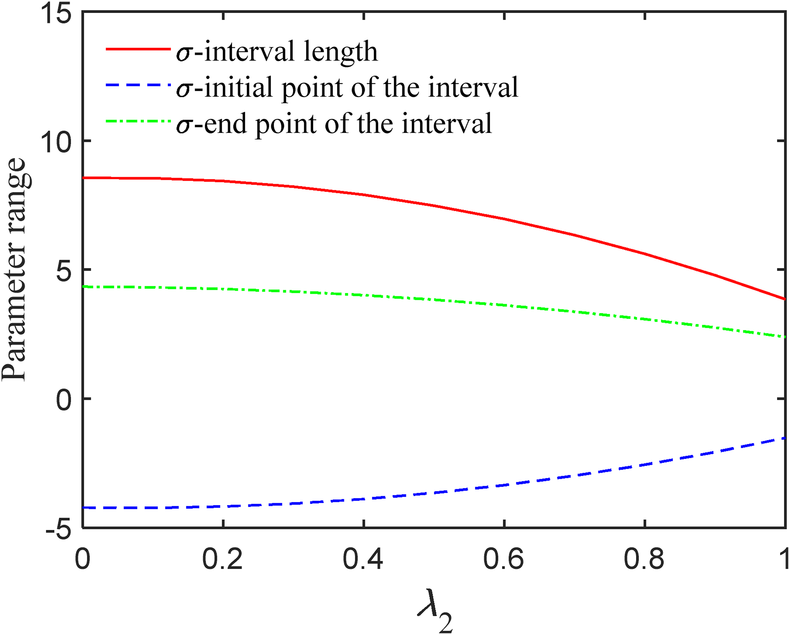

Table 2 and Figure 16 show that, to ensure system stability, as small a nonlinear damping coefficient as possible should be selected to increase the interval σ length of the frequency detuning parameter when the SMR exists. This maximizes the chance of the SMR in the nonlinear damping NES system.

Finally, the influence of the cubic stiffness coefficient on the interval σ existing in SMR is studied. By drawing the one-dimensional mapping diagram when cubic stiffness coefficient is 1.2, 0.5, and 0.8, respectively, the interval σ existing in SMR when the cubic stiffness coefficient changes is determined, as shown in Table 3:

Table 3.

The σ interval.

Cubic stiffness coefficient	σ Interval
λ₃ = 1.2	σ∈[−4.18, 4.25]
λ₃ = 1.5	σ∈[−4.47, 4.59]
λ₃ = 1.8	σ∈[−4.86, 4.92]

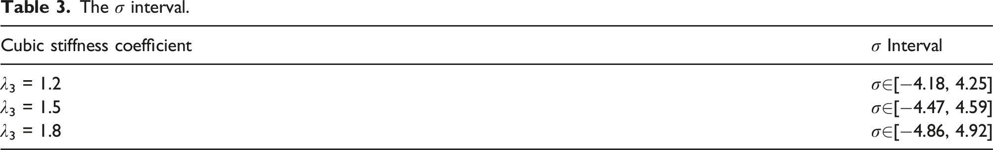
Table 3 shows that the length of the frequency detuning parameter interval increases with increasing cubic stiffness coefficient. The relationship between the two can be approximated by the quadratic function y = 0.5x²+0.75x+6.81. The initial points of the interval σ existing in the SMR decrease with increasing cubic stiffness coefficient, and the relationship between the two is approximated by the quadratic function y = −0.5556x²−0.5333x−4.02. The relationship between the end points of the interval σ existing in the SMR and the cubic stiffness coefficient is opposite to the initial points, and the relationship between the two is approximated by the quadratic function y = 0.2222x²+0.5x+3.33. The functional relationship between the interval length of the frequency detuning parameter, the initial points of the interval σ where the SMR exists, the end points of the interval σ where the SMR exists, and the cubic stiffness coefficient is shown in Figure 17.

Figure 17.

Diagram of different cubic stiffness coefficients and σ intervals.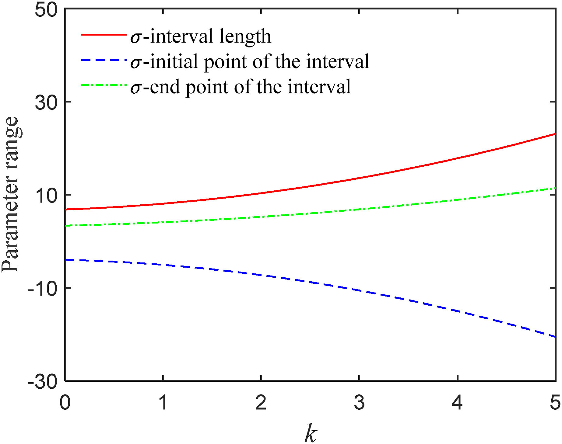

Table 3 and Figure 17 show that, to ensure system stability, as large a cubic stiffness coefficient as possible should be selected to increase the interval length of the frequency detuning parameter when the SMR exists. This maximizes the chance of the SMR in the nonlinear damping NES system.

The selected parameters are λ₂ = 0.2, λ₃ = 1.2, f = 3. The time-mileage diagram and the Poincare section of the system with and without SMR are drawn. As can be seen from in Figure 18, when the SMR phenomenon occurs in the system, the amplitude of the system can be greatly suppressed, so that the system can obtain better damping effect, and it is also proved that the rationality of the detuning parameter interval of the SMR through one-dimensional mapping analysis.

Figure 18.

Time-mileage diagram and Poincare sections of different σ.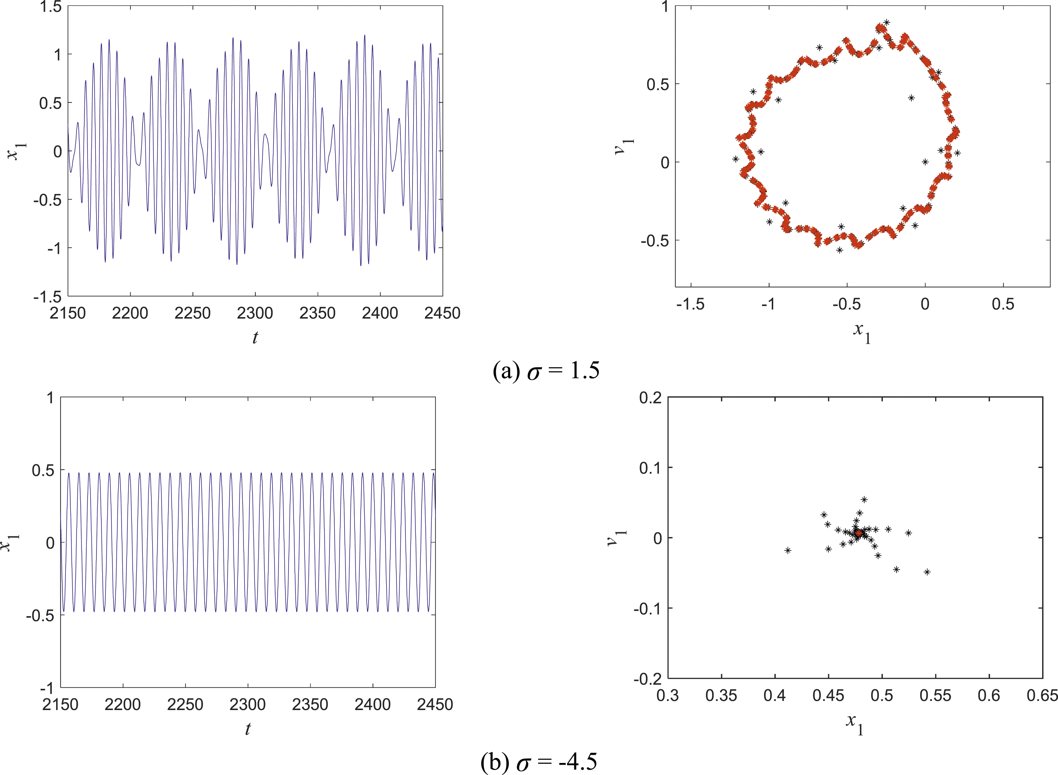

Conclusions

In this paper, the damping capability of nonlinear damping NES is analyzed, and the slow-varying equation of the system is derived using the complex variable average method and the multi-scale method. Firstly, the energy transfer efficiency analysis was carried out on the basis of the slow-change equation, and the condition: $\sqrt{3} ω^{3} λ_{2} \leq λ_{3}$ for the system to realize TET was derived, and the energy transfer equation was used to derive that the energy transfer efficiency keeps increasing with the increase of the cubic stiffness coefficient, and decreasing with the increase of the natural frequency. Secondly, the saddle-node bifurcation of the system is analyzed, and it is found that the shape of the saddle-node bifurcation boundary curve is approximately triangular, and it is also found that the frequency detuning parameter and the mass ratio will only affect the magnitude of the external excitation amplitude in the vertical coordinate, and have no effect on the nonlinear damping coefficient in the horizontal coordinate. Finally, the SIM diagram reveals that the jump phenomenon of different branches provides the basis for the existence of SMR, and analyzes the one-dimensional mapping to obtain a larger detuning parameter interval of SMR existence, which should be chosen as a smaller nonlinear damping coefficient, a larger amplitude of external excitation, and a larger cubic stiffness coefficient, and verifies that the analysis of the existence of detuned parameter interval of SMR existence by one-dimensional mapping is reasonable through the Poincare section and the time-mileage diagram.

Footnotes

Acknowledgments

The authors gratefully acknowledge the support of the National Natural Science Foundation of China through Grant No. 11872256.

Declaration of conflicting interests

The author(s) declared no potential conflicts of interest with respect to the research, authorship, and/or publication of this article.

Funding

The author(s) disclosed receipt of the following financial support for the research, authorship, and/or publication of this article: The authors gratefully acknowledge the support of the National Natural Science Foundation of China through Grant No. 11872256.

ORCID iDs

Xing-ke Qi

Jian-chao Zhang

Jun Wang

References

Asadi Jafari

Zarastvand

Zhou

. Doubly curved truss core composite shell system for broadband diffuse acoustic insulation. J Vib Control 2024; 30(17–18): 4035–4051.

Talebitooti

Zarastvand

Gheibi

. Acoustic transmission through laminated composite cylindrical shell employing third order shear deformation theory in the presence of subsonic flow. Compos Struct 2016; 157: 95–110.

Zarastvand

Ghassabi

Talebitooti

. Acoustic insulation characteristics of shell structures: a review. Arch Comput Methods Eng 2021; 28: 505–523.

Talebitooti

Zarastvand

. The effect of nature of porous material on diffuse field acoustic transmission of the sandwich aerospace composite doubly curved shell. Aero Sci Technol 2018; 78: 157–170.

Vakakis

Gendelman

Bergman

, et al. Nonlinear targeted energy transfer in mechanical and structural systems. Berlin: Springer Science & Business Media, 2008.

Xiong

Kong

Liu

. Influence of structural damping on a system with nonlinear energy sinks. J Vib Shock 2015; 34(11): 116–121. DOI: 10.13465/j.cnki.jvs.2015.11.021.

Barredo

Rojas

Mayén

, et al. Innovative negative-stiffness inerter-based mechanical networks. Int J Mech Sci 2021; 205: 106597.

Dekemele

De Keyser

Loccufier

. Performance measures for targeted energy transfer and resonance capture cascading in nonlinear energy sinks. Nonlinear Dynam 2018; 93: 259–284.

Kopidakis

Aubry

Tsironis

. Targeted energy transfer through discrete breathers in nonlinear systems. Phys Rev Lett 2001; 87(16): 165501.

10.

Wei

Peng

Dong

, et al. Mechanism of optimal targeted energy transfer. J Appl Mech 2017; 84(1): 011007.

11.

Liu

Tan

Chen

, et al. Strongly modulated response analysis of nonlinear energy sink absorption system under ground harmonic excitation. J Beijing Univ Technol 2019; 45(02): 177–185.

12.

Gendelman

Starosvetsky

Feldman

. Attractors of harmonically forced linear oscillator with attached nonlinear energy sink I: description of response regimes. Nonlinear Dynam 2008; 51: 31–46.

13.

Zhang

Kong

. Analysis on vibration suppression response of nonlinear energy sink with combined nonlinear damping. Chin J Theor Appl Mech 2023; 55(04): 972–981.

14.

Zang

Cao

Zhang

. Steady-state response of a viscoelastic beam with asymmetric elastic supports coupled to a lever-type nonlinear energy sink. Nonlinear Dynam 2021; 105: 1327–1341.

15.

Al-Shudeifat

. Nonlinear energy sinks with piecewise-linear nonlinearities. J Comput Nonlinear Dynam 2019; 14(12): 124501.

16.

Nguyen

Pernot

. Design criteria for optimally tuned nonlinear energy sinks—part 1: transient regime. Nonlinear Dynam 2012; 69: 1–19.

17.

Gourdon

Alexander

Taylor

, et al. Nonlinear energy pumping under transient forcing with strongly nonlinear coupling: theoretical and experimental results. J Sound Vib 2007; 300(3-5): 522–551.

18.

Zhang

Liu

Cao

, et al. Targeted energy transfer between 2-D wing and nonlinear energy sinks and their dynamic behaviors. Nonlinear Dynam 2017; 90: 1841–1850.

19.

Al-Shudeifat

. Time-varying stiffness method for extracting the frequency–energy dependence in the nonlinear dynamical systems. Nonlinear Dynam 2017; 89: 1463–1474.

20.

Gendelman

Gourdon

Lamarque

. Quasiperiodic energy pumping in coupled oscillators under periodic forcing. J Sound Vib 2006; 294(4-5): 651–662.

21.

Starosvetsky

Gendelman

. Bifurcations of attractors in forced system with nonlinear energy sink: the effect of mass asymmetry. Nonlinear Dynam 2010; 59: 711–731.

22.

Starosvetsky

Gendelman

. Vibration absorption in systems with a nonlinear energy sink: nonlinear damping. J Sound Vib 2009; 324(3-5): 916–939.

23.

Starosvetsky

Gendelman

. Response regimes in forced system with non-linear energy sink: quasi-periodic and random forcing. Nonlinear Dynam 2011; 64: 177–195.

24.

Kong

. Dynamics of 1-dof and 2-dof energy sink with geometrically nonlinear damping: application to vibration suppression. Nonlinear Dynam 2018; 91: 733–754.

25.

Geng

Ding

Mao

, et al. Nonlinear energy sink with limited vibration amplitude. Mech Syst Signal Process 2021; 156: 107625.

26.

Liu

Chen

Tan

. Dynamic analysis of the nonlinear energy sink with local and global potentials: geometrically nonlinear damping. Nonlinear Dynam 2020; 101: 2157–2180.

Research on energy transfer and vibration suppression of nonlinear energy sink with nonlinear damping

Abstract

Keywords

Introduction

Model statement of structure-nonlinear damping NES system

Analysis of energy transfer characteristics

Solve the system slow-varying equation

Slow invariant manifold analysis

Energy transfer efficiency analysis

Analysis of saddle-node bifurcation

Boundary equation derivation

Saddle-node bifurcation diagram of the system

SMR analysis of nonlinear damping NES system

Slow invariant manifold analysis under SMR

Analysis of the necessary conditions for SMR generation

Conclusions

Footnotes

Acknowledgments

Declaration of conflicting interests

Funding

ORCID iDs

References