Sage Journals: Discover world-class research

Abstract

Most machines are equipped with devices that monitor their operation. Air conditioners, in particular, are routinely monitored through various measurements. A desirable outcome of this monitoring is identifying when the device will likely require maintenance. In this study, we present the use of Ordinal Patterns, a symbolic transformation of time series, which allows for the visual assessment of the type of operation. Ordinal Patterns are chosen because they can transform intricate time series into simple and intuitive symbolic representations. The technique is visually appealing, generating points on a plane whose positions reveal hidden dynamics. This approach makes it easier to identify recurring or abnormal patterns in machine operations that may indicate wear or impending failure. Additionally, Ordinal Patterns allow for precise and understandable visualization of operational data, making interpreting results more accessible for professionals who may not be experts in data analysis. We compare two machines under different operational conditions with six measured variables. We analyze the expressiveness of the Ordinal Patterns and identify those variables that best differentiate the two machines. Furthermore, we incorporate machine learning algorithms, such as Artificial Neural Networks, Support Vector Machines, and Decision Trees, to evaluate and validate the effectiveness of Ordinal Patterns as discriminative features. Integrating machine learning methods with a symbolic transformation offers a robust approach for the early and accurate diagnosis of potential failures, enhancing the predictive maintenance of air conditioning equipment.

Keywords

Ordinal patterns machine learning compressors signals air conditioner rotor dynamics

Introduction

The increasing complexity of modern industrial systems poses significant challenges for monitoring and maintaining critical machinery, such as air conditioning compressors. Early fault detection and predictive maintenance are essential for operational continuity, energy efficiency, and sustainability. In this context, analyzing signals from air conditioning compressors using Ordinal Patterns is a promising approach to enhance the predictive accuracy of machine learning algorithms. This study explores the representativeness and effectiveness of Ordinal Patterns and machine learning algorithms.

Existing literature addresses various predictive maintenance techniques such as vibration, thermography, and oil analysis. However, as highlighted by Divya et al.,⁸ there needs to be more attention focused on the symbolic transformation of data and its application in machine learning algorithms. This study aims to fill this gap by investigating the effectiveness of Ordinal Standards and their potential to improve predictive accuracy, efficiency, and sustainability in air conditioning compressor maintenance.

We pose the following research questions:

RQ1 [Effect of Data Representation on Machine Learning Algorithm]: How does the use of encoded representations, derived from the Ordinal Patterns of signals collected from air conditioning compressors, influence the performance of machine learning models, particularly in the context of predictive maintenance and efficiency in industrial applications?

Our first research question examines how adopting Ordinal Patterns influences the performance of machine learning models, especially Neural Networks, within the context of predictive maintenance. We assess whether incorporating this representation into machine learning models can improve the detection of abnormal operating patterns and contribute to timely and less costly interventions.

RQ2 [Entropy-Complexity Analysis of Ordinal Patterns]: What insights can be gained from the analysis of the entropy (H) and complexity (C) from Ordinal Patterns regarding the classification of states of air conditioning compressors in industrial environments? How do these metrics correlate with the quality of machine classification?

The second research question analyses entropy (H) and complexity (C) metrics derived from Ordinal Patterns. We investigate the potential of these metrics to classify the compressor’s operational state and how they correlate with the accuracy of classifying the machine’s conditions. This implies understanding the compressors’ dynamics and how these metrics can capture subtle changes in their operations.

RQ3 [Comparison of Machine Learning Algorithms]: What is the comparative effectiveness of machine learning algorithms for machine state classification? Which algorithm excels in predictive accuracy, generalization, and computational efficiency?

This question explores the performance of various machine learning algorithms, from Decision Trees to more advanced models, in classifying compressor states. It aims to identify the most effective algorithm in terms of accuracy, generalization, and efficiency for compressor monitoring applications. The findings will inform future research and innovation in industrial maintenance and reliability engineering.

Related work

The Ordinal Patterns method proposed by Bandt and Pompe¹ is a technique for analyzing complex time series by computing symbols known as ordinal patterns based on the temporal ordering of data points in a time series. These patterns can be used to compute measures of disorder and complexity in the time series. The method has been broadly applied in various fields, including biomedicine, climatology, and the analysis of chaotic systems.¹⁹

Ordinal Patterns have revolutionized time series analysis by focusing on the rank order of values within small, overlapping windows rather than the values themselves. This approach transforms a time series into a sequence of symbols, enabling analyses based on their distribution. Its key advantages include robustness against outliers and invariance to monotonic data transformations, enhancing its appeal for diverse applications. The method effectively distinguishes between dynamical behaviors, from white noise to singular patterns in monotonic series. The seminal contribution by Bandt and Pompe¹ underlines the importance of pattern sequences, marking a significant shift towards understanding the underlying dynamics of time series.

Ordinal Patterns have been utilized to study the dynamics of chaotic lasers, market dynamics like the Libor market, atmospheric patterns, ecosystem productivity, transportation, energy consumption, and biomedical signals such as Electroencephalography (EEG) and Magnetoencephalography (MEG). These applications demonstrate the versatility of Bandt-Pompe’s methodology across different scientific and engineering domains.¹⁹ Mao et al.²⁰ extended Bandt and Pompe’s approach to multidimensional time series.

Ordinal patterns have significantly impacted machine diagnostics and monitoring across various equipment types and operational domains, providing early detection of potential failures and deepening the understanding of machines’ intrinsic characteristics. This methodology, as detailed in the work by Wang et al.,³⁴ has been pivotal in predictive maintenance, especially in analyzing machine signals for bearing failure detection. This approach has improved fault detection and isolation in complex machinery, including jet engines, by identifying anomalous vibration patterns. Wang’s research underscores the value of ordinal patterns in enhancing the reliability and efficiency of predictive maintenance strategies.

Several works have adopted a composite approach of analytical techniques to identify abnormal patterns that may indicate incipient failures in wind turbines and diesel engines. These studies have detected shifts in bearing vibration patterns through ordinal pattern analysis and permutation entropy, indicating potential future issues. Sharma³⁰ employs variational mode decomposition alongside permutation entropy for gear failure detection in complex and non-linear systems. This method merges instantaneous frequency estimation with ordinal pattern analysis, creating a powerful tool for anomaly identification.

The scope of signal analysis extends beyond turbines and engines, encompassing a variety of applications. Research efforts in fault diagnosis within steam turbine rotors³¹ have utilized Complete Ensemble Empirical Mode Decomposition with Adaptive Noise (CEEMDAN) alongside SVM-based methods to identify signatures characteristic of operational issues.

Combining the ordinal approach with machine learning techniques for model identification, time series classification, or forecasting is still challenging. The literature suggests that the properties of ordinal probabilities are not fully understood, and integrating these with machine learning remains an open problem.¹⁹ On May 29, 2024, a search for the terms “machine learning,” “ordinal patterns,” and “time series” on the Web of Science database yielded only four publications, highlighting the significance and relevance of the proposed study.

Other works² tackled the challenge of identifying and quantifying nonlinear temporal correlations in time series. They developed a method involving a machine learning algorithm trained to predict the temporal correlation parameter of flicker noise time series. They reduced the dimensionality of the feature space from numerous ordinal pattern probabilities to two features: the degree of stochastically and the strength of temporal correlations. Jiang et al.¹⁴ proposed an algorithm to identify self-correlations in stock prices using the concept of time series motifs, which are patterns that frequently appear within a time sequence. This approach utilized ordinal comparison and k-NN clustering to discover motifs to forecast stock temporal tendencies and prices.

Seddik et al.²⁹ integrated Weighted Permutation Entropy with a Support Vector Machine learning model to enhance the sensitivity and precision of automatic seizure detection in long-term scalp EEG data.

Guo et al.¹¹ proposed a Composite Multiscale Transition Permutation Entropy method to improve the feature extraction performance and robustness to noise for fault diagnosis in bearings. This method improved traditional Transition Permutation Entropy by considering the transition probability matrix of ordinal patterns at multiple scales.

The comprehensive review by Leyva et al.¹⁹ presents the evolution, applications, and ongoing challenges of the methods based on ordinal patterns.

Despite the advances in Ordinal Patterns, their integration with machine learning models for predictive maintenance of air conditioning compressors is little explored. This study applies Ordinal Patterns to that domain and evaluates their effectiveness on different machine learning algorithms. The innovation lies in combining symbolic transformation with advanced machine learning techniques, potentially enhancing operational efficiency, reducing maintenance costs and preventing unexpected failures in industrial environments.

Methodology

The entropy-complexity plane

Consider the time series of unique real values $X = (x_{1}, x_{2}, \dots, x_{T})$ of length T. We will transform small subsets of size D (the embedding dimension) into symbols. These subsets typically overlap and are not necessarily contiguous. The subset of dimension D whose first observation is x_t can be formed as

X_{t}^{(D, τ)} = (x_{t}, x_{t + τ}, \dots, x_{t + (D - 1) τ}),

(1)

where the integer τ ≥ 1 is the time delay, t = {1, 2, …, N} The vector

X_{t}^{(D, τ)}

is transformed into one D! possible symbols from the set π = {π⁽¹⁾, π⁽²⁾, …, π^(D!)}, typically through the rankings of its elements. With this, the time series

X

of length T is transformed into the sequence of symbols

P = (π_{1}, π_{2}, \dots, π_{N})

of length N = T − (D − 1)τ. For simplicity, this paper considers τ = 1.

Figure 1 shows two patterns of embedding dimension D = 3 and time delay τ = 1, namely $X_{1}^{(3,1)} = (x_{1}, x_{2}, x_{3})$ , and $X_{7}^{(3,1)} = (x_{7}, x_{8}, x_{9})$ . The rightmost pattern $X_{1}^{(3,1)}$ consists of increasing values. The indexes that sort them in increasing order are 1,2,3, so, its symbol could be called π₁ = π⁽¹²³⁾. The indexes that sort the leftmost pattern are 2,1,3. Therefore, its symbol could be called π₇ = π⁽²¹³⁾. The names are arbitrary as long as they uniquely identify each D! possible pattern.

Figure 1.

Two patterns of embedding dimension D = 3 and time delay τ = 1.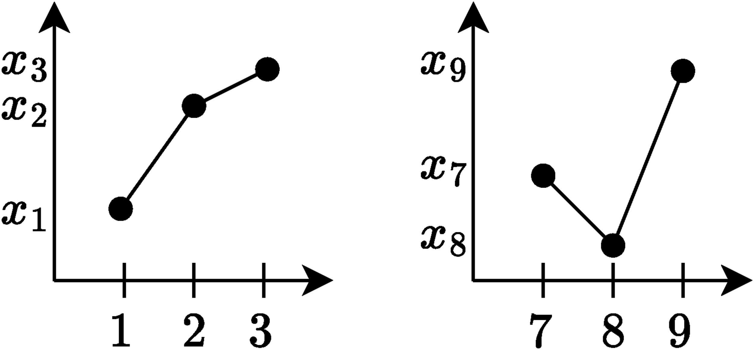

Once the complete time series $X = (x_{1}, x_{2}, \dots, x_{T})$ has been mapped onto N = T − (D − 1)τ patterns π = (π₁, π₂, …, π_N), we compute a histogram of proportions of symbols $h = {(h (j))}_{1 \leq j \leq D!}$ . This histogram estimates the probability distribution of patterns produced by the dynamics observed through $X$ . This histogram is used to extract descriptors from the time series.

An important descriptor is the Normalized Shannon Entropy, a measure of the system’s randomness, defined as:

H (h) = - \frac{1}{\log D!} \sum_{j = 1}^{D!} h (j) \log h (j),

(2)

where terms h(j) = 0 are omitted from the sum. This feature varies between 0 and 1, indicating either a single pattern or the uniform distribution of patterns, respectively, and is known as the “Permutation Entropy” (PE) of the series

X

Although the PE is expressive, it does not capture all the underlying dynamics of the time series. Lamberti et al.¹⁷ added the Jensen-Shannon distance between h and the uniform distribution $u = (1 / D!, 1 / D!, \dots, 1 / D!)$ to capture additional nuances:

Q^{'} (h, u) = \sum_{ℓ = 1}^{D!} [h (ℓ) \log \frac{h (ℓ)}{u (ℓ)} + u (ℓ) \log \frac{u (ℓ)}{h (ℓ)}] .

(3)

This value, termed “Disequilibrium,” is normalized as Q = Q′/ max{Q′}, where:

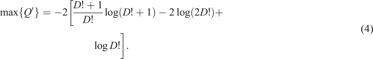
\begin{align} \max {Q^{'}} = - 2 [\frac{D! + 1}{D!} \log (D! + 1) - 2 \log (2 D!) + \\ \log D!] . \end{align}

(4)

Lamberti et al.¹⁷ used the product C = HQ as a measure of “Statistical Complexity” of the time series. Both H and Q are normalized, as is C. With this, we map a time series to a point in the H × C plane. Martin et al.²¹ obtained the edges of the closed manifold into which every possible time series is mapped.

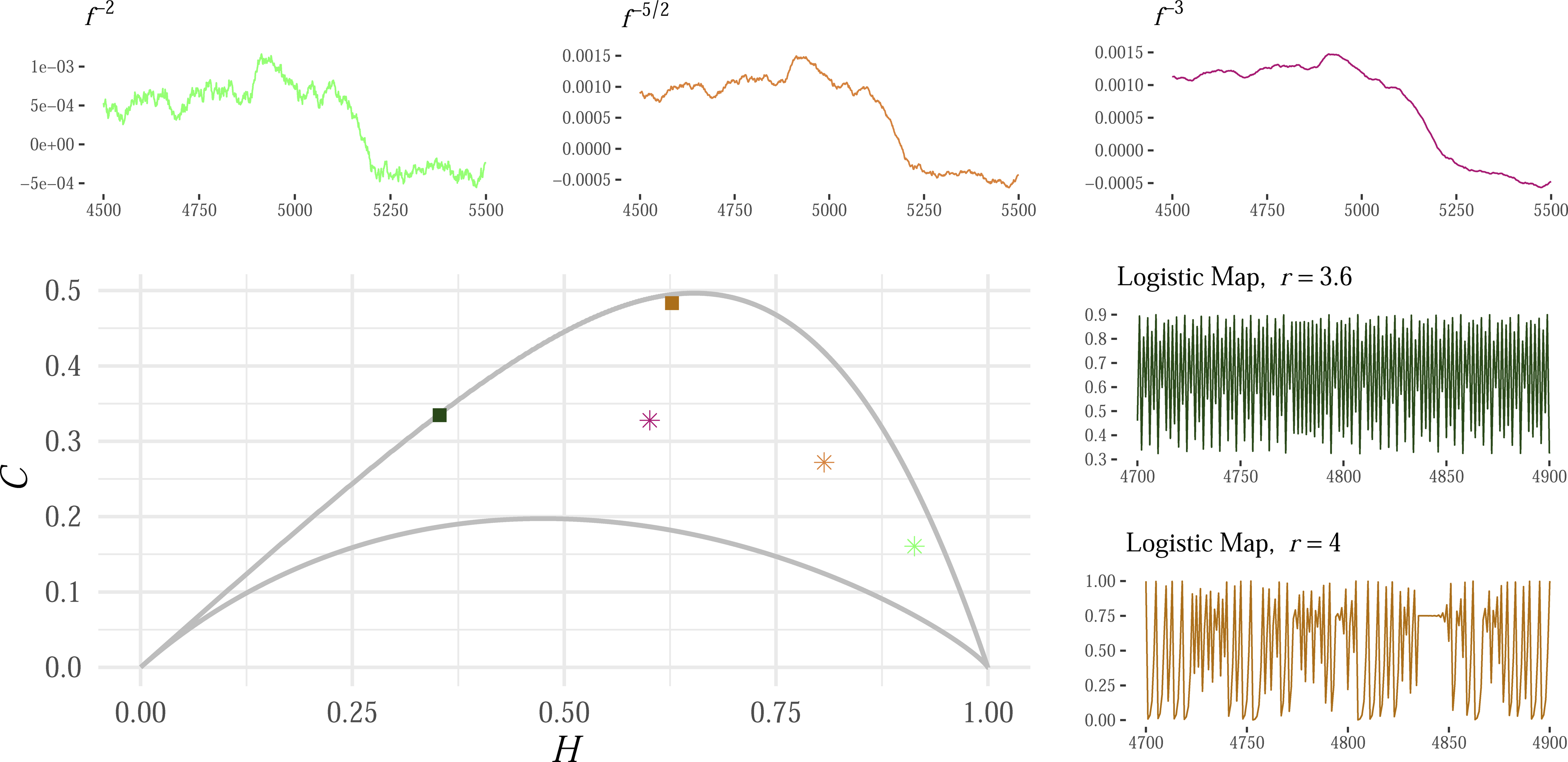
Figure 2 exemplifies mappings of deterministic functions and stochastic signals in the H × C plane, with an embedding dimension of D = 6. The point from each signal is depicted by a unique color. The two deterministic functions are logistic maps x_t = rx_t−1 (1 − x_t−1) with x₀ ∈ (0, 1), and r = 3.6 (green) and r = 4 (maroon). Their points have relatively low entropy and high complexity. The stochastic signals are 1/f ^k noise obtained by transforming the same white noise time series. We show the points of signals with k = −2 (light green), k = −5/2 (light maroon), and k = −3 (purple). They are increasingly correlated; the stronger the correlation, the smaller the entropy and the higher the complexity. This illustration highlights predictability and complexity differences between structured deterministic patterns and random stochastic signals.

Figure 2.

Several time series and their corresponding points in the Entropy-Complexity plane (H × C) for D = 6. Adapted from Chagas et al.⁵

Several freely available packages implement metrics derived from Ordinal Patterns. We have used the R package statcomp.³²

Our analysis uses six time series from two air conditioning compressors, as detailed in Table 1. These attributes are crucial for understanding the compressors’ performance, efficiency, and health, particularly in applications where precise temperature and pressure control is critical. These data are measurements over time in multiple dimensions, represented as “Att1” through “Att6.” We have the same attributes from a machine in working condition (“Good,” in teal in all plots) and a faulty machine (“Bad,” in red).

Table 1.

Measurements extracted from the two machines under study.

Attribute	Description
Att1	ADT: Air discharge temperature
Att2	Inlet temperature: Air intake temperature
Att3	Internal pressure
Att4	pN: System pressure
Att5	pNloc: System pressure (whole network)
Att6	Oil separator pressure differential

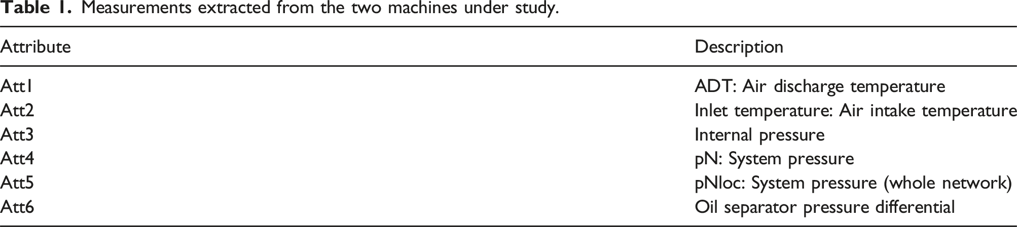
Figure 3 presents the points in the H × C plane of the six attributes from both machines using four embedding dimensions. We want to identify the best configuration for analyzing functional and malfunctioning states over various performance indicators.

Figure 3.

Visualization of all measures (“Att1” to “Att6,” one per column), machines (“Good” in teal and “Bad” in orange), embedding dimensions (3, 4, 5, and 6, one per row), and feasible bounds in the H × C plane.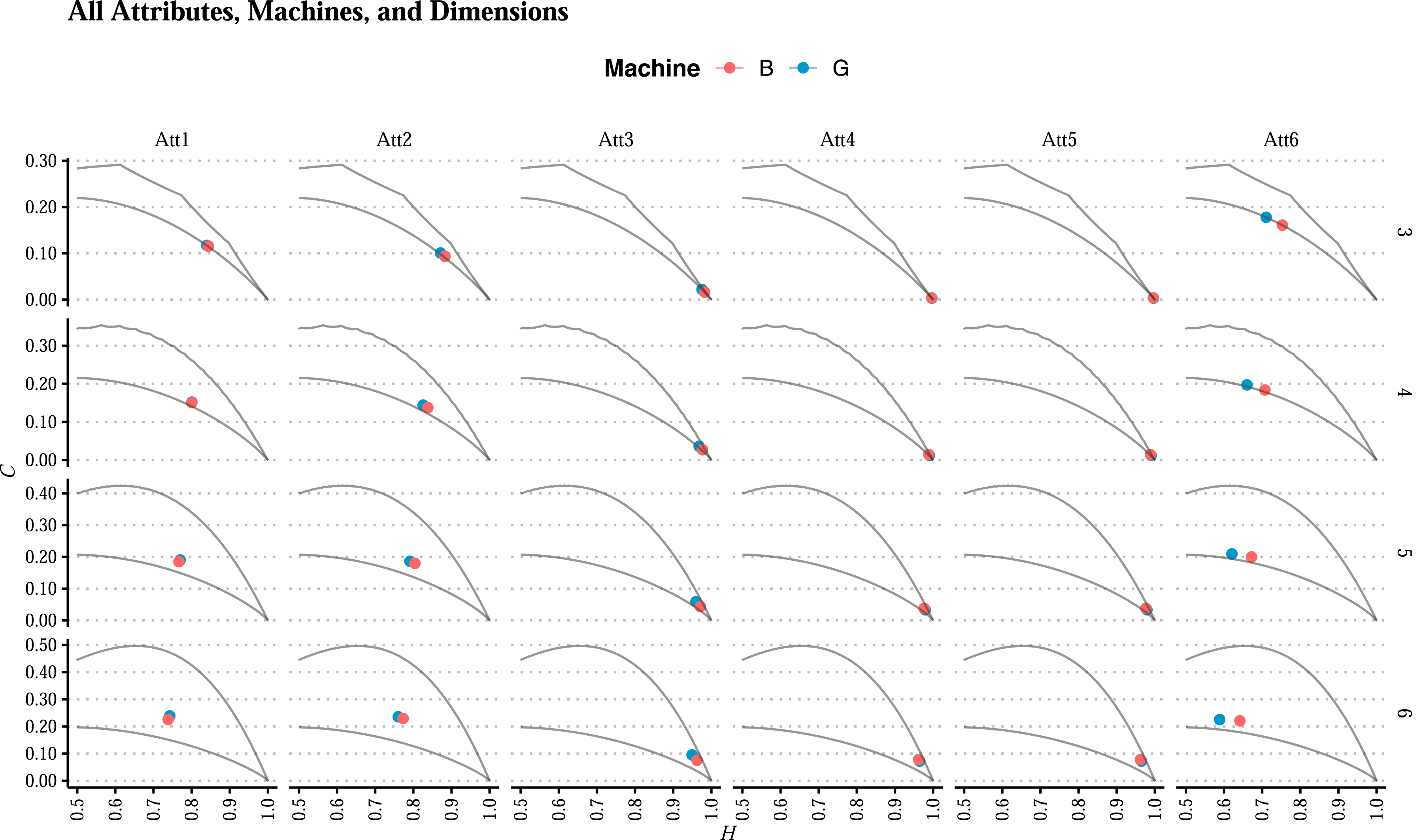

The approach here is to apply and evaluate machine learning models to classify time series data. The first scenario uses raw data directly, while the next stage improves upon this by adding the permutation entropy and complexity metrics. Different models, such as Neural Networks, SVMs, and Decision Trees, will be trained and tested. Performance will be evaluated by examining how well they classify when combining raw data and Ordinal Patterns metrics.

Feedforward neural networks

Feedforward Neural Networks (FNNs) are a fundamental machine learning architecture. The multilayer perceptron (MLP), a type of FNN, is known for modeling non-linearly separable data using fully connected layers of neurons with non-linear activation functions.²⁷ We explored their ability to discern between different patterns in data, serving as a complement to the previously discussed Entropy-Complexity plane. Thus, FNN maps the input data to a higher-level feature space, where the relationship between the data and the labels can be more easily discriminated.

An FNN’s architecture includes an input layer, one or more hidden layers, and an output layer. Learning within these networks is facilitated through the iterative adjustment of synaptic weights, employing the backpropagation algorithm in conjunction with gradient descent optimization techniques.²⁶

The weight adjustment process is expressed as:

Δ w_{j i} (n) = - η \frac{\partial E (n)}{\partial v_{j} (n)} y_{i} (n),

(5)

where η denotes the learning rate, w_ji are the weights,

E (n)

is the error at the output node, and v_j(n) and y_i(n) represent the weighted sum of the inputs and the output of the previous neuron, respectively.²⁶ The error at each output node j for the n the data point is given by e_j(n) = d_j(n) − y_j(n), with d_j(n) being the desired target value and y_j(n) the value produced by the network.²⁶ The global error function for a data point is:

E (n) = \frac{1}{2} \sum_{output node j} e_{j}^{2} (n) .

(6)

FNN’s capacity to learn complex patterns is attributed to the non-linearity introduced by the activation functions, which are propagated backwards during the weight update phase.¹⁸ We used the Adam optimizer, an extension of the stochastic gradient descent method, which adjusts the learning rate during training. The loss is calculated using binary cross-entropy, a common choice for binary classification problems. In binary classification contexts, the binary cross-entropy loss function is instrumental, defined as:

Loss = - \frac{1}{N} \sum_{i = 1}^{N} [y_{i} \log {\hat{y}}_{i} + (1 - y_{i}) \log (1 - {\hat{y}}_{i})],

(7)

with

{\hat{y}}_{i}

denoting the predicted output for input x_i and y_i the true label. Advanced variants of FNNs, like convolutional neural networks and radial basis function networks, diversify the activation functions to suit specific data distributions and task requirements better.

Table 2 lists various hyperparameters, which are critical values that can be adjusted to optimize the training process of a neural network. These values optimize our validation accuracy. The “Units in Layer 1” and “Units in Layer 2” rows suggest a network architecture with two dense layers. The given values (32, 64, and 128 for the first layer and 16, 32, and 64 for the second) indicate how many neurons are being experimented with in each layer. The “Learning Rate” is crucial for the convergence of the model during training, with values ranging from 0.001 to 0.1, showing a typical range from conservative to more aggressive learning. The “Training Epochs” and “Batch Size” rows specify the length of the training process and the number of samples to be passed through the network before the model’s weights are updated, respectively.

Table 2.

Hyperparameter configurations were tested for the Feedforward Neural Network model.

Hyperparameters	Values
Units in layer 1	32, 64, 128
Units in layer 2	16, 32, 64
Learning rate	0.001, 0.01, 0.1
Training epochs	10, 20, 30
Batch size	16, 32, 64
Early stopping strategy	3, 5, 7

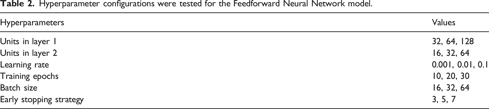
Lastly, the “Early Stopping Strategy” with values of 3, 5, and 7 suggests a mechanism to prevent overfitting by stopping the training if the model’s performance on a validation set does not improve for a specified number of epochs. Figure 4 illustrates validation error monitoring throughout training epochs, indicating an early stopping point. This visualization captures the moment when the training process stops to avoid overfitting based on the start of the validation error increase.

Figure 4.

Validation Error Trajectory with Early Stopping. The plot displays the validation error decreasing over epochs, followed by a rise indicating overfitting. The vertical dashed line represents the early stopping point, which was implemented to prevent the model from further overfitting the training data.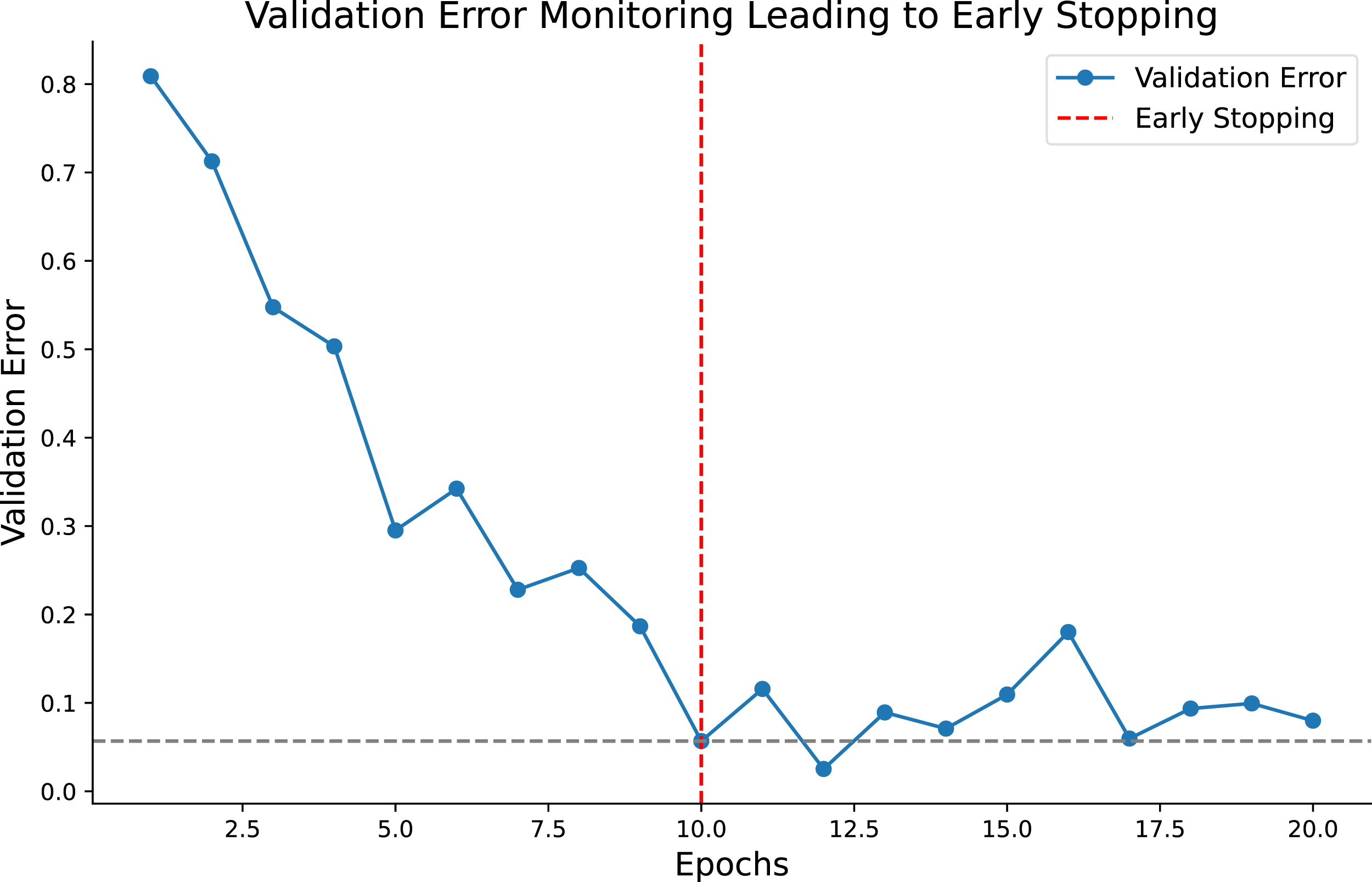

Network encoder

An Encoder Network is designed to transform high-dimensional input data into a lower-dimensional encoded representation.¹² This transformation involves a series of layers, each applying a non-linear function to the data, followed by dimensionality reduction. The Encoder Network is typically the first half of an Autoencoder architecture,⁹ the second half being the Decoder Network, which aims to reconstruct the input data from the encoded representation.

The process starts with the input layer, receiving the raw data. This data then passes through one or more hidden layers. Each layer applies a weight matrix, a bias vector, and a non-linear activation function, such as the Rectified Linear Unit ReLU or hyperbolic tangent tanh, to the input data:

h_{i} = f (W_{i} h_{i - 1} + b_{i}),

(8)

where h_i is the output of the i-th layer, h_i−1 is the output of the previous layer, W_i is the weight matrix, b_i is the bias vector, and f is the activation function.³³

The final layer of the Encoder outputs the encoded representation, commonly referred to as the bottleneck. This layer’s dimensionality is significantly smaller than the input layer, forcing a compressed data representation.

The Encoder Network’s training involves optimizing the weights and biases to minimize a loss function, typically using gradient descent methods.¹⁵ This function measures the reconstruction’s deviation from the original data provided by the Decoder Network.

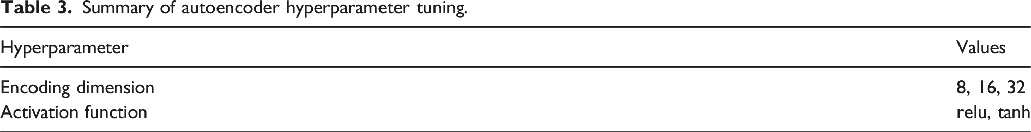
In our proposed methodology, we conduct an exhaustive hyperparameters search to optimize an Autoencoder neural network, which is critical for dimensionality reduction tasks. The objective is to identify the architecture that minimizes the validation loss, indicative of the model’s generalization capability.

The hyperparameters grid includes two essential parameters: the encoding dimension and the activation function, outlined in Table 3.

Table 3.

Summary of autoencoder hyperparameter tuning.

Hyperparameter	Values
Encoding dimension	8, 16, 32
Activation function	relu, tanh

Each model is compiled with the Adam optimizer and mean squared error loss function, conforming with the continuous nature of the input data. The training process incorporates a validation split and a EarlyStopping callback to prevent overfitting, as per the guidelines by Prechelt.²³

The performance of each model configuration is assessed based on the validation loss. If a new minimum validation loss is observed, the best model and its parameters are updated accordingly.

This approach ensures the derivation of an Autoencoder that is perfectly tuned to the idiosyncrasies of the input data, allowing for effective feature compression and reconstruction.

Support vector machines

Support Vector Machines (SVMs) are supervised learning methods for classification, regression, and outliers detection. The core idea behind SVM is to find a hyperplane in an N-dimensional space (N being the number of features) that distinctly classifies the data points. To separate two classes of data points, many possible hyperplanes could be chosen, but the goal is to find a plane with the maximum margin, that is, the maximum distance between data points of both classes.

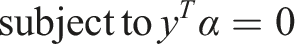
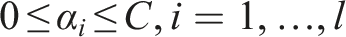
Formally, given training vectors $x_{i} \in R^{n}$ , i = 1, …, l in two classes, and a vector y ∈ {1,−1}^l, SVM solves the following primal problem:

\min_{w, b, ζ} \frac{1}{2} w^{T} w + C \sum_{i = 1}^{l} ζ_{i}

(9)

subject to y_{i} (w^{T} ϕ (x_{i}) + b) \geq 1 - ζ_{i},

ζ_{i} \geq 0, i = 1, \dots, l,

where w is the normal vector to the hyperplane, ϕ(x_i) denotes the feature-mapped input vectors, C is the penalty parameter of the error term, and ζ_i are the slack variables that allow misclassification of challenging or noisy examples.

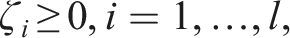
The dual problem is:

\min_{α} \frac{1}{2} α^{T} Q α - e^{T} α

(10)

subject to y^{T} α = 0

0 \leq α_{i} \leq C, i = 1, \dots, l

where e is the vector of all ones, C is the upper bound, Q is a l by l positive semi definite matrix, Q_ij ≡ y_iy_jK (x_i, x_j), and

K (x_{i}, x_{j}) = ϕ {(x_{i})}^{T} ϕ (x_{j})

is the kernel. Here, training vectors are implicitly mapped into a higher dimensional (possibly infinite-dimensional) space by the function ϕ.

The SVM algorithm outputs an optimal hyperplane that categorizes new examples. In the case of non-linearly separable input data, kernel functions, such as the Radial Basis Function (RBF), can transform the input space to a higher dimensional space where a hyperplane can be used to perform the separation.

For more details on the optimization and computation of SVM, readers are referred to the works by Cortes⁶ and Schölkopf and Smola.²⁸

Our study utilized an Autoencoder-Support Vector Machine (SVM) framework for classification tasks, leveraging the strengths of both methods. The Autoencoder encoded high-dimensional data into a lower-dimensional space, while the SVM classified the encoded data.

Combining autoencoders and support vector machines (SVM) is a powerful approach for classification and anomaly detection tasks. Autoencoders are neural networks that reduce the dimensionality of data, creating compact ²⁵ representations. These representations are then used to train an SVM, which can improve model performance, especially in anomaly detection tasks.²⁸

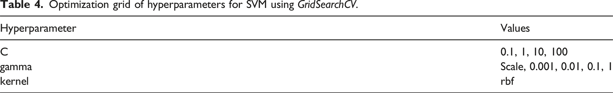
An SVM is a powerful supervised machine learning model that works by finding the optimal hyperplane that can best separate all the different classes with maximum margin. It uses kernel functions to transform the input space into a higher dimensional space where it is easier to perform the separation.⁶ (Tables 4 and 5).

Table 4.

Optimization grid of hyperparameters for SVM using GridSearchCV.

Hyperparameter	Values
C	0.1, 1, 10, 100
gamma	Scale, 0.001, 0.01, 0.1, 1
kernel	rbf

Table 5.

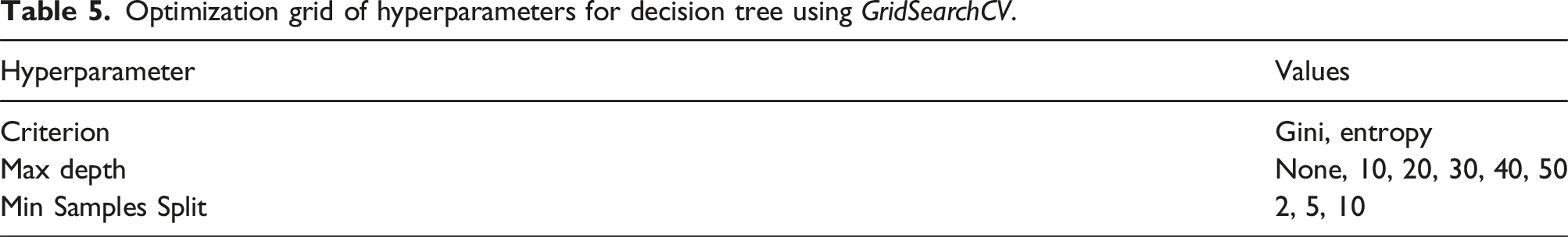
Optimization grid of hyperparameters for decision tree using GridSearchCV.

Hyperparameter	Values
Criterion	Gini, entropy
Max depth	None, 10, 20, 30, 40, 50
Min Samples Split	2, 5, 10

We encoded the normalized training and testing data using the best Autoencoder model from previous experiments. We employed GridSearchCV to optimize the SVM hyperparameters, exploring a range of values for C, gamma, and the kernel type:

Essentially, this technique exhaustively generates candidates from a grid of parameter values specified with the parameter. When fitting it to a dataset, all the possible combinations of parameter values are evaluated, and the best combination is retained.

The selection of hyperparameters C, gamma, and kernel for training a Support Vector Machine (SVM) is critical for model performance. According to Cortes,⁶ the C parameter balances classification accuracy with the decision function’s margin, and Hsu et al.¹³ recommend exploring a range of C values to find the best model. The gamma parameter^13,7 determines the reach of individual training examples, with scale often being a reasonable default value. Finally, the rbf kernel is chosen for its non-linearity and flexibility, characteristics essential for capturing complex patterns in high-dimensional data.²⁸

The SVM model was trained using the parameters grid to find the best hyperparameters.

The best SVM model discovered by the grid of parameters was evaluated on the test data. Performance metrics such as accuracy, recall, precision, and F1-score and a confusion matrix were calculated.

Decision tree

Decision Tree classifiers are a non-parametric supervised learning method for classification and regression. A Decision Tree aims to create a model that predicts the value of a target variable by learning simple decision rules inferred from the data features.

A decision tree is built by partitioning the input space recursively and defining a local decision boundary for each partition. A test is performed on a single feature to split the input space into two or more sub-spaces at each tree node. This process is known as recursive binary splitting in the context of binary trees. The feature and the threshold for splitting are selected based on a criterion that maximizes the difference between the sub-spaces in the target variable. Typical criteria include the Gini impurity, information gain, and variance reduction, which are intended to increase the homogeneity of the target variable within each subspace.⁴

Recursive partitioning continues until a stopping criterion is met, which could be the maximum depth of the tree, the minimum number of samples required to split a node, or a minimum gain in the splitting criterion. The resulting model is a tree that captures the decision-making process from the root to the leaves. Each leaf node corresponds to a decision outcome, the mode (for classification), or mean (for regression) of the target variable in that subspace.

The mathematical formulation for a binary decision tree can be expressed as a series of inequalities based on the feature values that lead to the decision outcomes. For a binary tree, a path from the root to a leaf can be represented as:

y = f (x) = \sum_{m = 1}^{M} c_{m} \prod_{j = 1}^{J_{m}} I (x_{π (j, m)} \leq t_{j, m})

(11)

where y is the predicted outcome, f(x) is the decision tree model, M is the number of leaf nodes, c_m is the outcome at the m-th leaf, J_m is the number of nodes from the root to the m-th leaf, x_π(j,m) is the feature at the j-th node in the path to the m-th leaf, t_j,m is the threshold at the j-th node, and I is the indicator function.

Decision Trees are widely used because they are interpretable, easy to use, and can handle numerical and categorical data. However, they are also prone to overfitting, which can be mitigated by pruning, setting minimum node size, or combining with ensemble methods like Random Forests.³

Configuring GridSearchCV for a decision tree involves specifying a dictionary of parameters, which maps the names of the parameters we want to optimize to the lists of potential values each parameter can take.

In this specific context, the parameter grid was defined with three keys corresponding to different hyperparameters of a decision tree:

We use GridSearchCV to generate combinations of these values to train and validate multiple decision trees through a cross-validation procedure.) will use combinations of these values to train and validate multiple decision trees through a cross-validation procedure. Each parameter combination will perform a cross-validation process with a specified number of folds (partitions of the dataset), assessing the accuracy of each resulting model. The goal is to identify the parameter combination that yields the best average cross-validation performance, thus balancing the model’s accuracy with its ability to generalize to unseen data.

The best model is updated based on these metrics. If the current model outperforms the previously recorded best model in terms of accuracy or F1-score, it becomes the new best model.

This methodology allows us to refine our model selection based on quantifiable performance metrics iteratively, ensuring we retain the most effective classifier for our predictive tasks.

Nature of time series data

We analyzed time series data collected from air conditioning compressors. Six characteristics were measured, as shown in Table 1.

The datasets encompass measurements tracked over time and span a range of dimensions, identified as “Att1” through “Att6.” These characteristics were captured from machinery in two distinct operational states: one functioning optimally, indicated by teal in all visual representations, and the other exhibiting malfunctions, shown in red. Figure 5 illustrates these details, displaying the distribution of each attribute alongside the condition status of the machines.

Figure 5.

Temporal Evolution of Attributes across machines: Time Series Comparison of “Good” and “Bad” Machines for Each Attribute “Att1” through “Att6.” The best candidates for discrimination in the H × C plane are “Att3” and “Att6” (right column).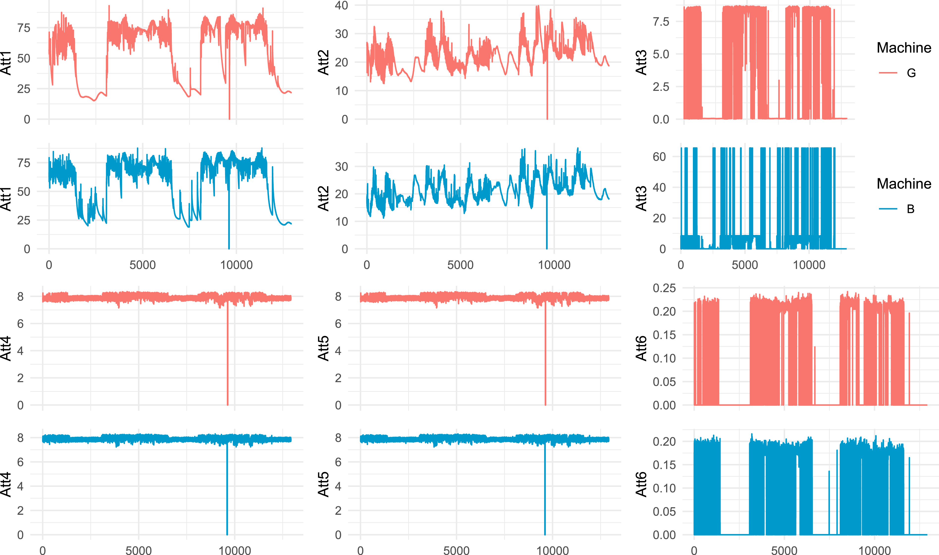

The analysis of the temporal evolution of six attributes from air conditioning compressors reveals distinct operational patterns between the working and malfunctioning machines. Attributes “Att1” (air discharge temperature) and “Att2” (inlet temperature) show significant fluctuations in malfunctioning machines, indicating possible issues in refrigeration or cooling systems. “Att3” (internal pressure) is highly discriminative, with abrupt spikes in malfunctioning machines. In contrast “Att4” and “Att5” (system pressures) show similar, consistent patterns. “Att6” (oil separator pressure differential) also stands out, with significant variations in malfunctioning machines.

Through the temporal evolution analysis of attributes from both machines, a comparative time series for each characteristic, “Att1” through “Att6,” was established. Notably, the attributes “Att3” and “Att6” (Figure 3) emerged as the most distinguishing attributes when comparing the performance in the H × C plane of machines classified as “Good” and “Bad.”

Data scenarios and experimental setup

From the time series data of the two machines, we created two scenarios to apply our machine learning algorithms, and details can be seen in Figure 6.

Figure 6.

Illustration of “Scenario I” and “Scenario II”: key feature vector components with time series data attributes indicator.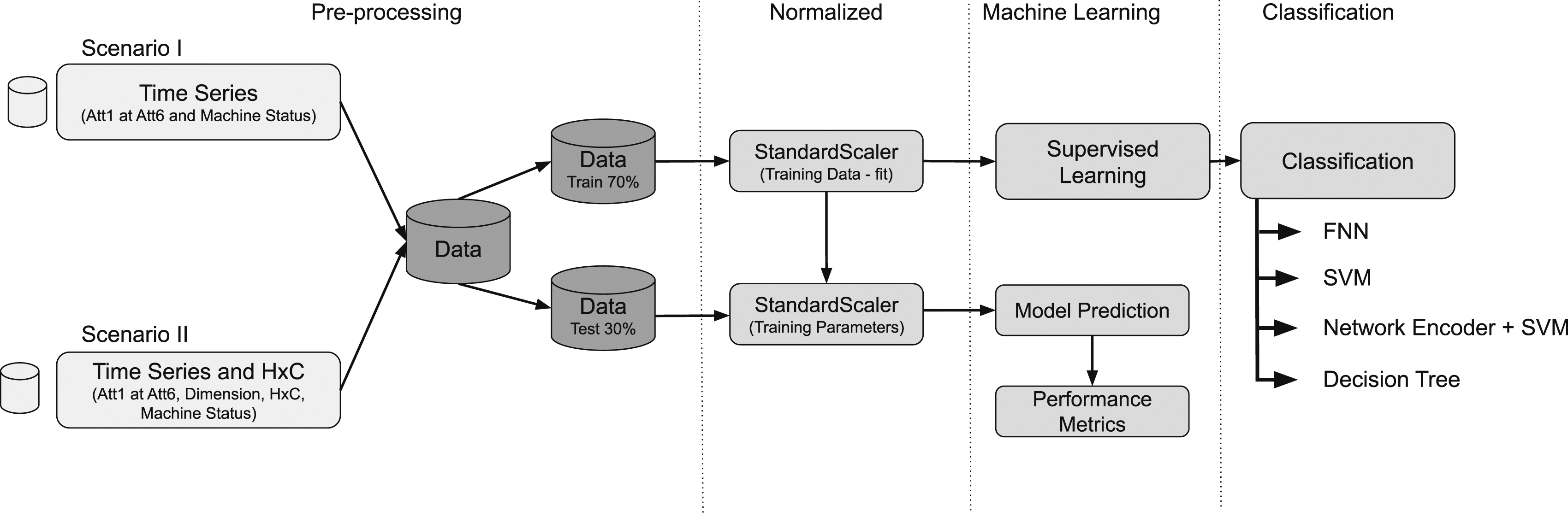

The figure outlines a machine learning workflow for data analysis, divided into two data input scenarios, preprocessing and supervised learning for classification:

• Scenario I (Traditional Characteristics): time series data comprising attributes from “Att1” to “Att6” and the machine status are collected. This scenario focuses solely on the direct analysis of the time series data.

• The Scenario II: it encapsulates the integration of both traditional time series data and Entropy-Complexity (H × C) metrics, which include entropy (H), complexity (C), dimension, and machine status. This consolidated approach allows for a multifaceted analysis, aiming to uncover patterns within the data that are not immediately visible through simple observation of the time series alone. By combining the detailed attributes of raw time series data with the nuanced insights provided by entropy and complexity metrics, this scenario offers a comprehensive perspective designed to enhance classification accuracy. It represents a synthesis of methodologies, leveraging the strengths of traditional data analysis alongside advanced metrics to facilitate a deeper understanding of the underlying dynamics within the dataset.

Each of these data scenarios undergoes a preprocessing process involving normalization of the data by subtracting the sample mean and dividing by the sample standard deviation. Such normalization is a common practice in data analysis and statistical modeling. It helps to address issues related to the scale of variables and ensures that all variables have the same importance when building statistical models.

Data is collected and stratified at the preprocessing stage into training (70 %) and testing (30 %) sets. During preprocessing, these data scenarios undergo normalization to ensure consistency and comparability among variables. Normalization is performed using the “StandardScaler” technique, which adjusts the data to have a mean of zero and a standard deviation of one. This involves centering the data by subtracting the mean and scaling it by the standard deviation of each numerical feature.

These transformations are crucial in statistical modeling, mitigating problems that arise from differences in variable scales.⁷

After normalization, the training data undergoes fitting with the StandardScaler. This step is essential for the correct model application and is indicated by “Training Data-fit.” Subsequently, the parameters derived from the training set are applied to normalize the test set, a process indicated by “Training Parameters.” This practice ensures that the test normalization aligns with the training parameters, preserving the integrity of the modeling process.

The module of Machine Learning - The normalized training data is used for supervised learning. This stage is pivotal for the model to learn mapping inputs to expected outputs and is represented by the transition from StandardScaler (Training Data - fit) to “Supervised Learning.” After training, the trained model is used to make predictions on the normalized test set, as illustrated by the transition to “Model Prediction.” Consequently, performance metrics are calculated based on these predictions, an essential step to assess the model’s efficacy.

The supervised learning process culminates in classification, which is the primary goal of the model’s training. Various classification methods are explored, such as:

• FNN (Feedforward Neural Network): A neural network that moves data in only one direction (forward) from input to output.

• SVM (Support Vector Machine): A machine learning model that seeks the best hyperplane to separate the data classes.

• Network Encoder + SVM: A combination that may involve transforming the data through a network encoder before classification via SVM.

• Decision Tree: A model that uses a tree-like structure for decision-making based on the characteristics of the data.

Each of these classification techniques is applied post-supervised learning, allowing for comparing their effectiveness for the specific dataset at hand.

For Scenario I, the dataset comprises 9050 instances of “Good” machines and 9048 instances of “Bad” machines for the training set. The testing set consists of 3879 cases for both “Good” and “Bad” machines. In Scenario II, the dataset contains 217,207 instances of “Good” machines and 217,173 cases of “Bad” machines for the training set. The testing set includes 93,089 instances of “Good” machines and 93,075 cases of “Bad” machines.

Figure 6 presents a machine learning methodology that includes preprocessing and supervised classification, with different data input scenarios that can enhance the accuracy of classifying machines based on their operational status.

The computational infrastructure for training the algorithms includes a MacBook Air (Model Identifier MacBook Air 10,1) equipped with an Apple M1 chip with eight cores (four performance and four efficiency cores). The machine has 8 GB of memory, storage capacity of 245.11 GB, and runs on macOS Ventura 13.3.

Results

In Scenario I Table 6, the evaluation of machine learning models on time-series data for air conditioning systems presents a comprehensive picture of their diagnostic capabilities. The attributes considered—air discharge temperature (ADT), air intake temperature, internal pressure, system pressure (pN), system pressure across the whole network (pNloc), and oil separator pressure differential—are critical parameters that reflect the operational health of air conditioning units.

Table 6.

Comparison of model performances of scenarios I and II (LR: Learning rate and BS: Batch size).

Model type	Accuracy (%)	Recall (%)	Precision (%)	F1-score (%)	Training time (s)	Best parameters
Scenario I
Feedforward neural networks	82.00	77.86	84.86	81.20	10.17	Units1: 64, Units2: 32, LR: 0.01, epochs: 20, BS: 32, Patience: 5
SVM	80.27	70.51	87.60	78.13	398.43	C: 100, gamma: Scale, kernel: rbf
Network encoder with SVM	80.32	70.66	87.57	78.21	408.33	C: 100, gamma: Scale, kernel: rbf
Decision tree	94.37	94.37	94.44	94.36	4.95	Criterion: Entropy, max depth: 10, min samples split: 2
Scenario II
Feedforward neural networks	98.54	99.91	97.24	98.56	270.92	Units1: 32, Units2: 16, learning rate: 0.001, epochs: 10, batch size:: 16, Patience: 3
SVM	99.97	99.97	99.97	99.97	28300063,2	C: 10, gamma: 1, kernel: rbf
Network encoder with SVM	99.97	99.97	99.97	99.97	18791179,2	C: 10, gamma: 1, kernel: rbf
Decision tree	100.00	100.00	100.00	100.00	55.49	Criterion: Gini, max depth: None, min samples split: 2

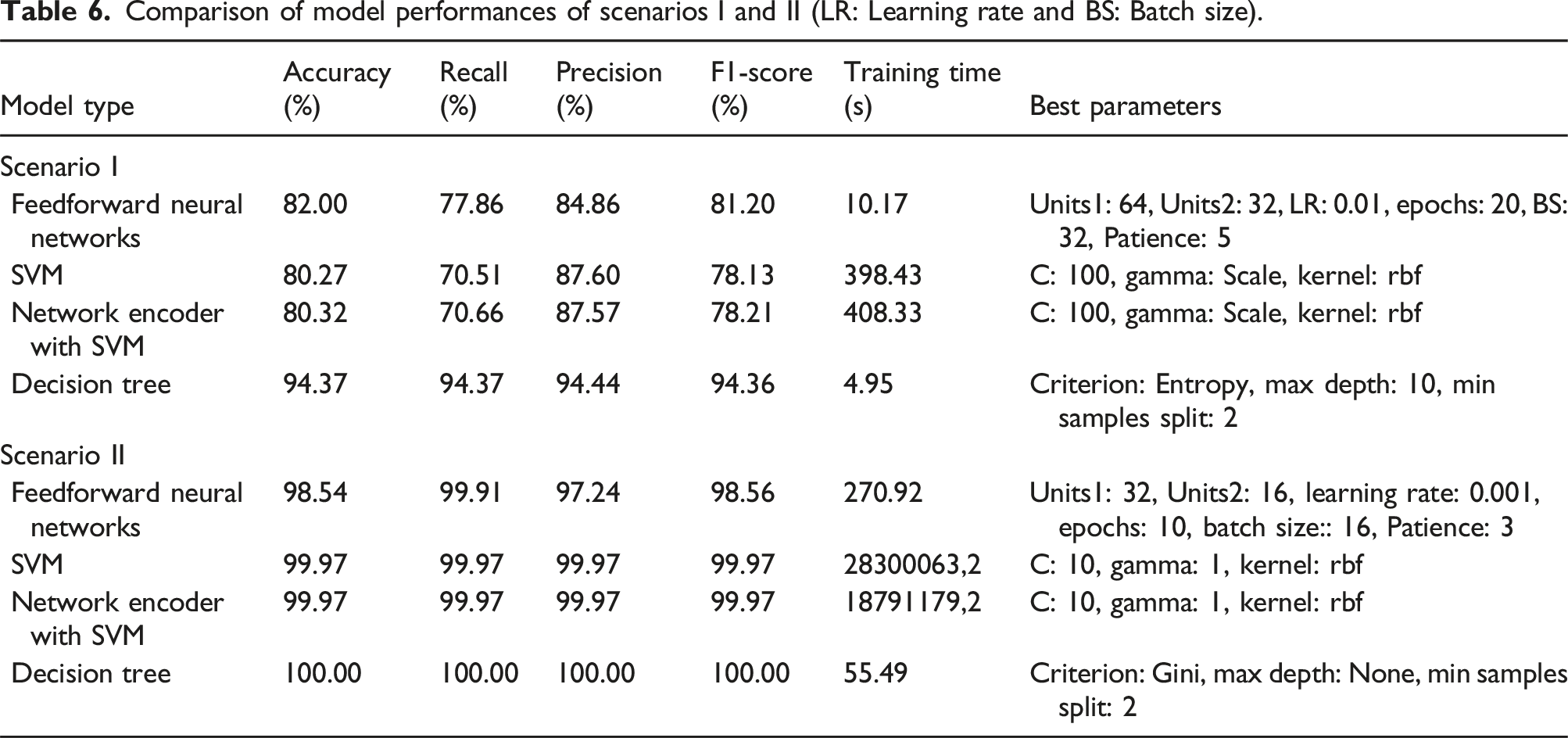
The Decision Tree model demonstrated superior performance with accuracy and F1-Score of 94.37 %, indicating high precision and reliability in distinguishing between faulty and well-functioning machines. This is consistent with literature suggesting decision trees are adept at handling non-linear relationships typical in time-series data, characterized by temporal dependencies and variable interactions.¹⁶

Feedforward Neural Networks showed commendable performance, with accuracy slightly above 82 %. Neural networks are known for their ability to model complex patterns, but their performance can be sensitive to the choice of architecture and hyperparameters.¹⁰ The moderate performance in this scenario could suggest a need for further tuning or a more complex network structure to capture the dynamics of the time-series data more effectively.

Deqiang Zou and Hongtao Man propose a hybrid algorithm that integrates a Support Vector Machine (SVM) with a neural network, specifically using an Autoencoder. The authors argue that the depth of a convolution neural network should be aligned with human perception levels and propose a model where the initial part of an Autoencoder acts as the kernel function for the SVM, which is the central classifier. This model aims to combine the strengths of each component, potentially improving performance in tasks such as COVID-19 detection.³⁵

The SVM and Network Encoder with SVM models, as analyzed by Zou and Man,³⁵ have demonstrated accuracies around 80 %, which falls short of the Decision Tree model’s performance. This relative underperformance of SVM models may be attributed to their design principle, which excels when handling data with distinct separability. Given the nuanced patterns present in time-series data from air conditioning systems—where variables like temperature and pressure interact in intricate ways—a linear separation approach may not be optimal, as these patterns could challenge the hyperplane-based separation mechanism inherent in SVMs.

Interestingly, while the Network Encoder with SVM took significantly longer to train due to the encoding process, it did not substantially improve accuracy. This outcome suggests that the encoding process may not have been able to extract more useful features from the time-series data or that the SVM is not the best model to leverage the encoded features.

In terms of practical applications, the ability to accurately predict machinery faults using these attributes can lead to proactive maintenance strategies. For example, anomalies in ADT and inlet temperature may indicate compressor issues or refrigerant problems, while unusual pressure readings might suggest blockages or leaks.²² The high precision and recall of the Decision Tree model suggest it could be a valuable tool for maintenance teams to prevent downtime and extend the lifespan of air conditioning units.

In summary, the results from Scenario I show the importance of choosing an appropriate machine learning model that aligns with the characteristics of time-series data. Moreover, they highlight the potential of decision trees in industrial diagnostics, reaffirming their role in predictive maintenance frameworks within the literature.

The confusion matrices of Figure 7 displayed in shades of sky blue offer valuable insights into each classification model’s performance for diagnosing air conditioning systems based on time-series attributes.

Figure 7.

Scenarios I and II - Confusion Matrices for HVAC System Fault Diagnosis: Each subplot represents the classification outcomes of a different machine learning model. The shades of sky blue indicate the count of true positives (top left), false negatives (bottom left), false positives (top right), and true negatives (bottom right), with darker shades corresponding to higher counts. The labels “True” and “False” correspond to the model’s correct or incorrect predictions, respectively.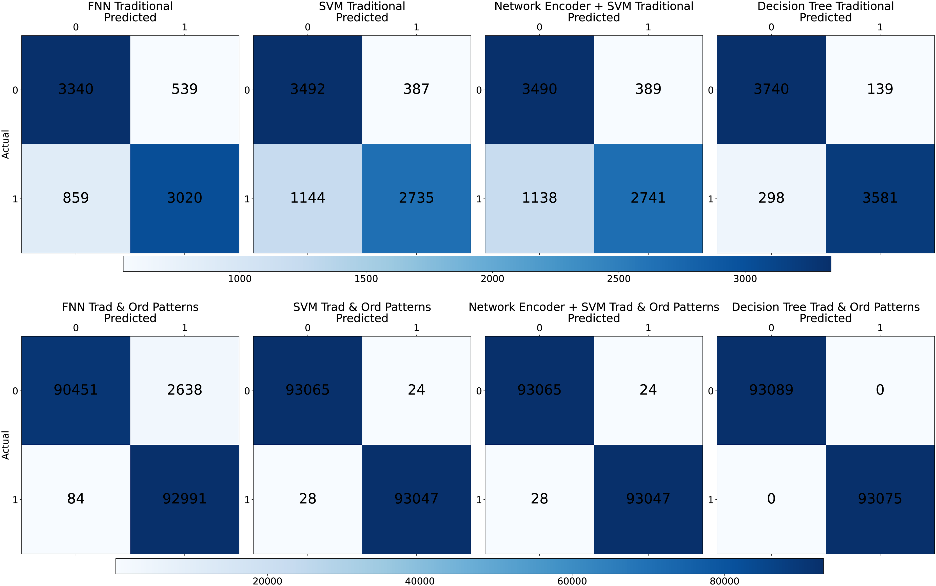

For Figure 7 the Feedforward Neural Networks, the confusion matrix indicates a substantial number of true positives (TP = 3340) and true negatives (TN = 3020), suggesting that the model is quite adept at identifying both faulty and non-faulty machines. However, with false negatives (FN = 859) and false positives (FP = 539), there is room for improvement, particularly in reducing the type II error (FN), which in practical terms means reducing the instances of undiagnosed faulty conditions.

The SVM model shows a high precision with fewer false positives (FP = 387), meaning it is less likely to label a non-faulty system as faulty. However, the higher number of false negatives (FN = 1144) compared to the Feedforward Neural Networks suggests that while it is reliable in its positive predictions, it might miss more faulty systems, not flagging them when it should.

Network Encoder with SVM yielded results similar to the standalone SVM regarding true positives and negatives but with slightly higher false positives (FP = 389) and slightly fewer false negatives (FN = 1138). The minimal differences between SVM and Network Encoder with SVM suggest that the encoding process did not significantly enhance the SVM’s ability to distinguish between the classes in this case.

The Decision Tree model is the most accurate among all models, evidenced by the highest number of true positives (TP = 3740) and true negatives (TN = 3581) and the lowest counts of false positives (FP = 139) and false negatives (FN = 298). This suggests an excellent balance between sensitivity (ability to identify faulty systems) and specificity (ability to identify non-faulty systems). Such performance makes the Decision Tree model particularly suitable for reliable diagnostics, minimizing both the risk of false alarms and the danger of missed fault detections.

In a real-world scenario, false negatives can be costlier than false positives because a missed diagnosis might lead to a system failure. In contrast, a false alarm would only lead to an unnecessary inspection. Therefore, the Decision Tree model’s low FN rate indicates its potential to reduce maintenance costs and prevent downtime in air conditioning systems, asserting its suitability for deployment in predictive maintenance applications within the Heating, Ventilation, and Air Conditioning (HVAC) industry as the models created in Scenario I.

In Scenario II, the application of Machine Learning models to air conditioning systems showed excellent results. The Feedforward Neural Networks (FNN), incorporating both Traditional and Ordinal Patterns, achieved an accuracy of 98.54 % with an impressive recall of nearly 100 %, indicating its robustness in correctly identifying system statuses. Despite taking longer to train, the FNN’s performance was notable for its precision and F1-Score. On the other hand, both SVM and Network Encoder with SVM attained a near-perfect accuracy, recall, precision, and F1-Score of 99.97 %. However, their training times were significantly longer, particularly for the SVM, which was the most extended. The Decision Tree model achieved perfection across all metrics, with an accuracy, recall, precision, and F1-Score of 100 %, coupled with a remarkably short training time. The confusion matrices further validated the effectiveness of these models, especially the Decision Tree, in providing reliable diagnostics for predictive maintenance.

As illustrated in Figure 8, the “Decision Tree Trad & Ord Patterns” model showed a highly favorable balance between the True Positive Rate (TPR) and the False Positive Rate (FPR), practically reaching the ideal point (0.1) in the ROC-like graph, indicative of a perfect classification ability without any false positives. The “FNN Trad & Ord Patterns” and “Network Encoder + SVM Trad & Ord Patterns” models also showed excellent performances, with high TPRs and low FPRs, highlighting their effectiveness in the task of classifying the operational states of air conditioning systems. In comparison, the traditional “FNN,” and “SVM” models delivered commendable performances, albeit with a slightly higher FPR, resulting in a slightly higher false positive rate.

Figure 8.

ROC-like Plot of TPR versus FPR for Models—This plot displays the comparative performance of various machine learning models on the task of classifying operational states of air conditioning systems. The True Positive Rate (TPR) is plotted against the False Positive Rate (FPR) for models trained on traditional data, ordinal patterns, and a combination of both. The dashed line represents a random chance classifier.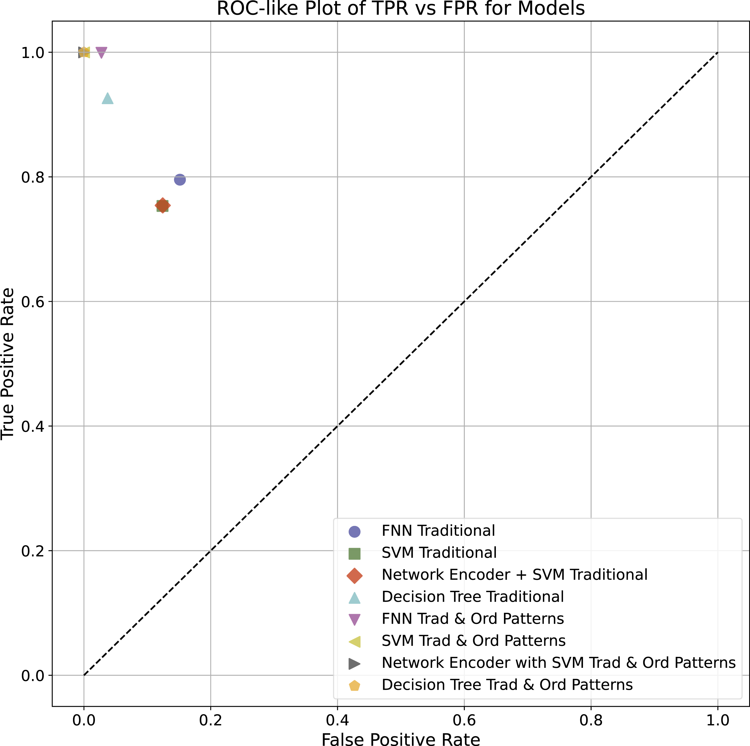

In the same traditional context, the Network Encoder with the SVM Traditional model demonstrates a performance parallel to the SVM Traditional. This observation implies that the network encoding phase may not have substantially enhanced the SVM’s discrimination power for the dataset.

Focusing on models trained solely on ordinal patterns, there is a noticeable divergence in effectiveness. The Decision Tree model maintains a substantial equilibrium in performance metrics, whereas the SVM model points to a higher FPR, signaling a potential area for improvement.

Performance significantly improves when we turn to models that integrate traditional and ordinal pattern features. Excluding the FNN, all models achieve a TPR near unity alongside an FPR approaching zero, underlining a highly precise classification prowess with minimal false positives.

Figure 8 supports the advantages of blending traditional and ordinal pattern approaches. Across all examined scenarios, the Decision Tree models stand out for their performance, reinforcing their adaptability and potential as robust classifiers for such tasks. This figure also highlights the importance of model selection and feature representation in machine learning tasks. The results indicate a promising direction for future research, particularly in exploring the fusion of traditional and complex data representations for improved classification accuracy in predictive maintenance.

In response to the research questions:

RQ1: The study’s findings suggest that integrating Ordinal Patterns of features significantly improves the performance of Neural Networks. This advancement facilitates enhanced detection of faults in air conditioning compressors, contributing to more effective predictive maintenance strategies.

RQ2: Insights from the entropy and complexity metrics, based on Ordinal Patterns, are instrumental in distinguishing the operational states of air conditioning compressors. The metrics exhibit a strong correlation with the classifiers’ ability to accurately identify the condition of the machines, indicating their impact on the quality of machine classification.

RQ3: Comparative analysis of machine learning algorithms highlights the outstanding performance of Decision Trees in predictive accuracy, generalization, and computational efficiency. Its superiority over other models in classifying compressor states makes it the tool of choice for industrial applications, especially in compressor monitoring.

Conclusions

This study examined various machine learning models for diagnosing the operational health of air conditioning compressors, focusing on the integration of Ordinal Patterns. The “Decision Tree Trad & Ord Patterns” model consistently demonstrated the highest classification accuracy, efficiency, and generalization ability, achieving perfect scores in accuracy, recall, precision, and F1-Score in Scenario II. The integration of Ordinal Patterns significantly improved the performance of the models, with “FNN Trad & Ord Patterns” and “Network Encoder + SVM Trad & Ord Patterns” also showing high True Positive Rates (TPR) and low False Positive Rates (FPR).

Traditional Feedforward Neural Networks (FNN) and Support Vector Machines (SVM) delivered commendable performances but had slightly higher FPRs, indicating increased rates of false positives. This suggests that these models may benefit from further tuning or more complex network structures to better capture the dynamics of the time-series data. Accurately predicting machinery faults using key attributes can lead to proactive maintenance strategies. The high precision and recall of the Decision Tree model underscore its potential as a valuable tool for maintenance teams, helping to prevent downtime and extend the lifespan of air conditioning units.

The relative underperformance of SVM models compared to Decision Trees may be due to their design principle, which excels in handling data with distinct separability. Given the nuanced patterns in time-series data from air conditioning systems, a linear separation approach may not be optimal. The findings emphasize the importance of selecting appropriate machine learning models that align with the characteristics of the data. The incorporation of Ordinal Patterns significantly enhances model performance, particularly for Decision Trees, making them highly suitable for industrial diagnostics and predictive maintenance frameworks.

Future work will extend these methodologies, employing advanced neural network architectures or exploring the potential of unsupervised learning techniques to uncover even more nuanced patterns within the data, and using the statistical properties of the features from ordinal patterns.²⁴ The artifacts of this work can be found at the following link: https://github.com/keilabcs/Compressors-Ordinal-Patterns.

Footnotes

Declaration of conflicting interests

The author(s) declared no potential conflicts of interest with respect to the research, authorship, and/or publication of this article.

Funding

The author(s) received no financial support for the research, authorship, and/or publication of this article.

ORCID iDs

Keila Barbosa

Alejandro C Frery

References

Bandt

Pompe

. Permutation entropy: a natural complexity measure for time series. Phys Rev Lett 2002; 88(17): 174102.

Boaretto

Budzinski

Rossi

, et al. Evaluating temporal correlations in time series using permutation entropy, ordinal probabilities and machine learning. Entropy 2021; 23(8): 1025.

Breiman

. Random forests. Mach Learn 2001; 45(1): 5–32.

Breiman

Friedman

Olshen

, et al. Classification and regression trees. Boca Raton, FL: Chapman and Hall/CRC, 1984.

Chagas

ETC

Queiroz-Oliveira

Rosso

, et al. White noise test from ordinal patterns in the Entropy-Complexity plane. Int Stat Rev 2022; 90(2): 374–396. DOI: 10.1111/insr.12487.

Cortes

Vapnik

. Support-vector networks. Mach Learn 1995; 20(3): 273–297.

de Amorim

Cavalcanti

Cruz

. The choice of scaling technique matters for classification performance. Appl Soft Comput 2023; 133: 109924.

Divya

Marath

Santosh Kumar

. Review of fault detection techniques for predictive maintenance. J Qual Mainten Eng 2023; 29(2): 420–441.

Goodfellow

Bengio

Courville

. Deep learning. Cambridge, MA: MIT Press, 2016. https://www.deeplearningbook.org

10.

Goodfellow

Bengio

Courville

. Deep learning. Cambridge, MA: MIT Press, 2016.

11.

Guo

Zou

, et al. Composite multiscale transition permutation entropy-based fault diagnosis of bearings. Sensors 2022; 22(20): 7809.

12.

Hinton

Salakhutdinov

. Reducing the dimensionality of data with neural networks. Science 2006; 313(5786): 504–507.

13.

Hsu

C-W

Chang

C-C

Lin

C-J

, et al. A practical guide to support vector classification, 2003.

14.

Jiang

Y-F

C-P

Han

J-Z

. Stock temporal prediction based on time series motifs. 2009 International conference on machine learning and cybernetics 2009; 6: 3550–3555.

15.

Kingma

Welling

. Auto-encoding variational bayes. Ithaca, NY: arXiv, 2013.

16.

Kumar

Thenmozhi

. Forecasting stock index movement: a comparison of support vector machines and random forest. In: Indian Institute of Capital Markets 9th Capital Markets Conference Paper, Mumbai, India, 2006.

17.

Lamberti

Martín

Plastino

, et al. Intensive entropic non-triviality measure. Phys Stat Mech Appl 2004; 334(1–2): 119–131. DOI: 10.1016/j.physa.2003.11.005.

18.

LeCun

Bengio

Hinton

. Deep learning. Nature 2015; 521(7553): 436–444.

19.

Leyva

Martínez

Masoller

, et al. 20 years of ordinal patterns: perspectives and challenges. Europhys Lett 2022; 138(3): 31001. DOI: 10.1209/0295-5075/ac6a72.

20.

Mao

Shang

. Multivariate multiscale complexity-entropy causality plane analysis for complex time series. Nonlinear Dynam 2019; 96: 2449–2462.

21.

Martin

Plastino

Rosso

. Generalized statistical complexity measures: geometrical and analytical properties. Physica A 2006; 369: 439–462. DOI: 10.1016/j.physa.2005.11.053.

22.

Morimoto

Hashimoto

Ohtomo

, et al. Development of diagnostic method for air conditioning equipment using wavelet transform. Build Eng 2005; 111(2): 667–674.

23.

Prechelt

. Early stopping — but when? Neural Network: Tricks of the Trade 1998; 7700: 55–69.

24.

Rey

Frery

Gambini

, et al. Asymptotic distribution of entropies and Fisher information measure of ordinal patterns with applications. Chaos, Solit Fractals 2024; 188: 115481. DOI: 10.1016/j.chaos.2024.115481.

25.

Rifai

Vincent

Muller

, et al. Contractive auto-encoders: explicit invariance during feature extraction. In: Proceedings of the 28th International Conference on International Conference on Machine Learning. Madison, WI: Omnipress, 2011, pp. 833–840.

26.

Rumelhart

Hinton

Williams

. Learning representations by back-propagating errors. Nature 1986; 323(6088): 533–536.

27.

Schmidhuber

. Deep learning in neural networks: an overview. Neural Network 2015; 61: 85–117.

28.

Schölkopf

Smola

. Learning with kernels: support vector machines, regularization, optimization, and beyond. Cambridge, MA: MIT Press, 2001.

29.

Seddik

Youssef

Kholief

. Automatic seizure detection in long-term scalp eeg using weighted permutation entropy and support vector machine. In: 2014 Cairo International Biomedical Engineering Conference (CIBEC). Piscataway, NJ: IEEE, 2014, pp. 170–173.

30.

Sharma

. Gear fault detection based on instantaneous frequency estimation using variational mode decomposition and permutation entropy under real speed scenarios. Wind Energy 2021; 24(3): 246–259. DOI: 10.1002/we.2570.

31.

Shi

Z-B

C-X

Cao

L-H

, et al. Study of the diagnosis of the faults occurred to the rotor of a steam turbine based on the CEEMDAN (complete ensemble empirical mode decomposition with adaptive noise) and CBBO-SVM (biogeography-based optimization with chaos-supporting vector machine). Reneng Dongli Gongcheng/Journal of Engineering for Thermal Energy and Power 2018; 33(1): 69–74. DOI: 10.16146/j.cnki.rndlgc.2018.01.011.

32.

Sippel

Lange

Gansstatcomp

: Statistical complexity and information measures for time series analysis, 2019. R package version 0.1.0. Available at: https://CRAN.R-project.org/package=statcomp

33.

Vincent

Larochelle

Lajoie

, et al. Stacked denoising autoencoders: learning useful representations in a deep network with a local denoising criterion. Journal of Machine Learning Research 2010; 11: 3371–3408.

34.

Wang

Tang

, et al. Injury identification of wind turbine bearing based on issd and 1.5 dimension envelope order spectrum under variable rotating speed condition. Taiyangneng Xuebao/Acta Energiae Solaris Sinica 2021; 42(1): 240–247. DOI: 10.19912/j.0254-0096.tynxb.2018-0811.

35.

Zou

Man

. A novel perspective towards svm combined with autoencoder. J Phys : Conf Ser 2022; 2347(1): 012011. DOI: 10.1088/1742-6596/2347/1/012011.

Analysis of signals from air conditioner compressors with ordinal patterns and machine learning

Abstract

Keywords

Introduction

Related work

Methodology

The entropy-complexity plane

Feedforward neural networks

Network encoder

Support vector machines

Decision tree

Nature of time series data

Data scenarios and experimental setup

Results

Conclusions

Footnotes

Declaration of conflicting interests

Funding

ORCID iDs

References