Sage Journals: Discover world-class research

Abstract

This research investigated the feasibility of applying hardware order-tracking (HOT) and segmentalized amplitude normalization (SAN) to enhance the diagnosis of multiple bearing defects at different levels under varying rotation speeds. The vibration of operating bearings may present an energy variation phenomenon due to different levels of bearing defects, while the fluctuation of vibration amplitude may be attributable to changes in rotation speeds. These two factors inevitably interfere with each other when diagnosing bearing defects at multiple levels and classes under varying rotation speeds. In this paper, the research focuses on conducting an in-depth analysis of signal signatures, followed by providing a physical insight into feature extraction. Consequently, it enables the application of simple machine learning methods to accurately diagnose various bearing defects, even when dealing with significantly different patterns in training and testing data due to varying rotation speeds. To verify the effectiveness of the proposed SAN method for cases involving varying rotation speeds, the training and testing sets used datasets (vibration measurements) corresponding to different rotation speed profiles. The experimental and analytical results revealed that the proposed SAN method can normalize datasets with disparate vibration patterns, and alleviate the coupling of vibration energy variation and shaft rotation speed. This enhancement resulted in approximately 18.6% increase in the accuracy of bearing diagnosis for cases involving varying rotation speeds.

Keywords

Bearing defect segmentalized amplitude normalization order tracking varying rotation speed empirical mode decomposition instantaneous order marginal order spectrum

Introduction

A manufacturing process is typically expected to operate continuously; thus, the arrangements related to the maintenance of mechanical components play a vital role in manufacturing engineering. Bearings, as integral components of rotating machinery, significantly influence the operational performance of a system. Bearings can experience degradation due to various factors (such as material fatigue, inadequate lubrication, excessive load, and issues during manufacturing and assembly). When the bearings of rotating machinery malfunction, they may result in undesired vibrations and be detrimental to the performance and precision of machines. Therefore, addressing bearing defects is an important task and a prevalent challenge in industrial machinery. Given that the vibration characteristics provide insights into the dynamic state of a system, the combined utilization of vibration signal analysis and intelligent machine learning has been widely adopted for bearing fault diagnosis. This approach enables effective identification and resolution of bearing issues due to their impact on vibration behavior.

Numerous studies have explored bearing fault diagnosis and demonstrated the feasibility of vibration signal analysis for detecting defective bearings.^1,2 In general, the feature extraction techniques employed in bearing fault diagnosis mainly encompass the utilization of measured signal processing in both the time domain^3,4 and frequency domain.^5,6 Because of the cyclic and impact-based vibration behavior of defective bearings, envelope analysis has been employed to assess bearing condition and diagnose bearing defects.^6,7 Given the non-stationarity nature of vibration signals obtained from defective rotary systems, various forms of time-frequency analyses have been employed for processing measured data and extract features related to defective bearings. Examples include wavelet transform–based methods^8–11 and Hilbert–Huang transform–based methods.^12–15 These techniques have been applied to facilitate the monitoring and diagnosis of bearing conditions by capturing relevant features associated with defective bearings.

Studies have employed various methods to validate the feasibility and effectiveness of vibration-based bearing fault diagnostics. However, the majority of these studies have focused on cases involving fixed or steady rotation speeds. It is worth noting that the bearing rotation mechanism signifies that the principal features of operational bearings are influenced by the characteristic frequencies originating from the shaft rotation speed. To address situations involving varying shaft rotation speeds due to variable loads, order-tracking techniques have been applied to remove the rotation speed factor and normalize the characteristics of rotary systems.^16–19 Computed order-tracking methods, due to their compatibility with general vibration measurements, have been widely utilized for conducting fault diagnosis in rotating machinery.^20,21 Alternatively, Wu et al.²² proposed an instantaneous dimensionless frequency normalization scheme for the detection of gear faults, particularly in scenarios where rotation speeds vary.

With the rapid advancement of machine learning and artificial intelligence technology, researchers are increasingly harnessing data-driven methods and intelligent tools for bearing fault diagnosis.^23–26 Support vector machines (SVMs) have been employed as classifiers in studies focused on diagnosing various bearing faults in rotating machinery.^9,15 These classification tools have been adept at identifying flaws on the inner race, outer race, and roller of roller bearings. Lin et al.²⁷ optimized the SVM parameters using an artificial fish-swarm algorithm, while Saha et al.²⁸ utilized the particle swarm optimization (PSO) technique to enhance SVM hyperparameter tuning and thereby improve bearing fault diagnosis the performance. Various neural networks have also been utilized for detecting diverse bearing defects. Additionally, Chuya-Sumba et al.²⁹ applied a 1-D CNN-based deep learning method to diagnose the bearing condition of a high-speed machining (HSM) center, demonstrating elevated computational efficiency and diagnostic accuracy. In the realm of industrial geared motors, an adaptive neurofuzzy inference system, alongside statistical indicators, was employed for automated diagnostics of ball bearing defects.³⁰

Furthermore, it is well-recognized that the entropy can serve as a valuable metric for estimating the complexity of a system. Hence, a range of entropy computations, including sample entropy,³¹ approximate entropy,³² permutation entropy,^33,34 and energy entropy,³⁵ have been employed to evaluate regularity or disorderliness inherent in vibration measurements. There entropy-based approaches prove instrumental not only in dynamics identification but also in the realm of fault diagnosis.

Recently, a Vold–Kalman order-tracking technique was utilized for mechanical fault detection in vehicle motors.³⁶ This research addressed bearing faults, rotor eccentricity fault, and compound faults in permanent magnet synchronous motors under variable working conditions by applying the Vold–Kalman filter. Jiang et al.³⁷ proposed a tacholess order-tracking method to obtain rotation speeds based on spectral amplitude modulation (SAM), capable of diagnosing bearing faults at variable rotation speeds. Additionally, Goyal et al.^38,39 used a non-contact sensor to acquire vibration data for bearing health monitoring and fault diagnosis, avoiding the physical connection of vibration measurement to the machine test stand. They employed principal component analysis (PCA) and sequential floating forward selection (SFFS) for feature dimension reduction and feature selection under different loads and speeds. A three-dimensional hybrid fusion neural network (3D-HFB) was presented for diagnosing composite bearing faults.⁴⁰ Their approach, consisting of multivariate variational mode decomposition (MVMD) and an improved three-dimensional convolution neural network (3D-CNN), performs both data- and feature-level fusion of multi-phase motor current signals from a public dataset with an electromechanical drive system.

The order-tracking technique possesses the capability to transform vibration signals into a data format characterized by identical angular increments, thereby removing the influence of rotation speed variations. In the realm of fault diagnosis involving fluctuating shaft rotation speeds, numerous studies have employed the computed order-tracking technique to normalize characteristic frequencies in relation to rotation speed. The application of this technique necessitates the utilization of complicated interpolation schemes^18–20 or sophisticated algorithms (such as the Vold–Kalman filter³⁶), facilitating the reconstruction of vibration measurements to align with fixed angular displacements. Furthermore, as emphasized in Ref. 37, access to synchronous rotation speed information is imperative for the successful reconstruction of angle-domain signals. Compared with studies in Refs. 36 and 37, the hardware order-tracking (HOT) technique utilized in this research does not require sophisticated computation processes and rotation speed information. The accelerometers used for vibration measurement in HOT are generally compatible and inexpensive (such as MEMS sensors) with versatile applications in industrial machinery, even though they need to be physically attached to the test stand, unlike the non-contact sensor used in Refs. 38 and 39. Furthermore, the vibration accelerations acquired by accelerometers typically contain higher frequency oscillation information than motor current signals,⁴⁰ which may be crucial for extracting critical machine signatures in the high-frequency band.

It is acknowledged that varying rotation speeds induce fluctuations in vibration energy within faulty running bearings. Simultaneously, disparate levels of defects within bearings can also contribute to variations in vibration energy during operation. Consequently, the interplay of these two factors amplifies the challenge of effectively identifying diverse levels of multiple defects under varying rotation speeds.

In an effort to tackle the aforementioned issues and enhance bearing fault diagnosis for scenarios involving varying rotation speeds, the current study proposes the utilization of a segmentalized amplitude normalization (SAN) method for processing extracted features. This is accomplished by employing HOT measurements. The HOT application allows for precise recording of angle-domain signals, bypassing the need for conventional numerical interpolation schemes. Consequently, the characteristic frequencies of defective bearings are represented in terms of characteristic orders, regardless of the shaft’s rotation speed. The research focuses on conducting an in-depth analysis of signal signatures to provide physical insight into feature extraction. Therefore, it enables the application of simple machine learning methods to improve the accuracy of diagnosing various bearing defects, even when dealing with significantly different patterns in training and testing data due to varying rotation speeds.

A bearing test rig was employed to validate the efficacy of the proposed method in diagnosing various classes and levels of bearing defects under four rotation speed profiles. This research delves into a comprehensive analysis of signal feature extraction. The goal is to enhance diagnostic accuracy through the application of straightforward machine learning techniques, even in instances of diverse bearing defects. This challenge is compounded by highly different patterns in training and testing data due to varying rotation speeds.

To address this, a basic SVM classifier was employed to discern the extracted features from multiple levels and classes of defective bearings. This process also highlights the improvement in diagnosis achieved through the application of the SAN method. Analysis of the experimental results from the present study unveils that the proposed SAN method effectively mitigates the interference caused by varying rotation speeds and variations in vibration energy. Consequently, the values of the extracted features exhibit enhanced concentration and consistency due to the diminished influence of rotation speed. For the SVM utilized in this study, training sets were chosen from data sets corresponding to one of four rotation speed profiles. Correspondingly, testing sets were obtained from the data sets of the remaining three rotation speed profiles. This design ensures that the vibration pattern in the training data greatly differs from that of the testing data, facilitating a robust evaluation of the effectiveness of the SAN method. The outcomes of the diagnostic process from the current experiment affirm that the accuracy of diagnosing various levels and classes of bearing defects witnesses substantial enhancement with the implementation of the proposed SAN method. The signals recorded during this experiment are accessible on a cloud drive, providing further opportunities for reference and application.⁴¹

Vibration measurement and signal analysis

Experimental setup

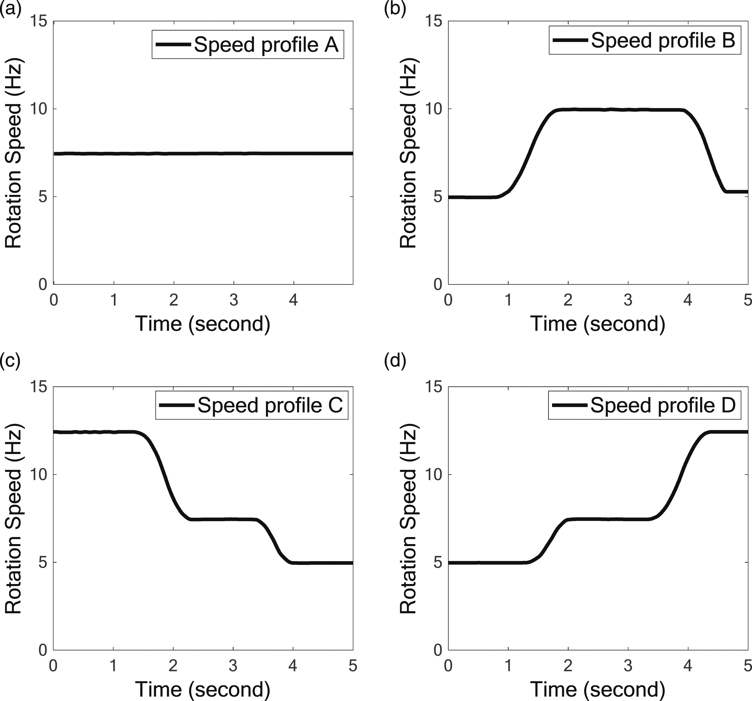
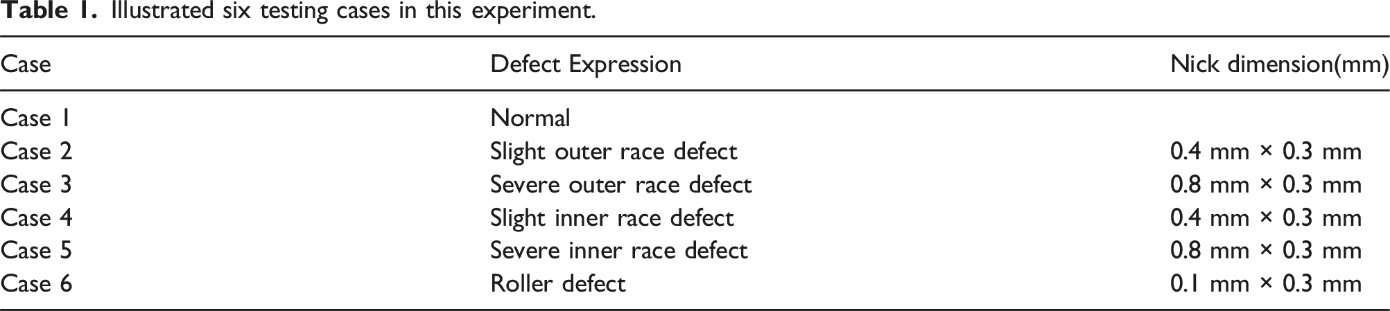
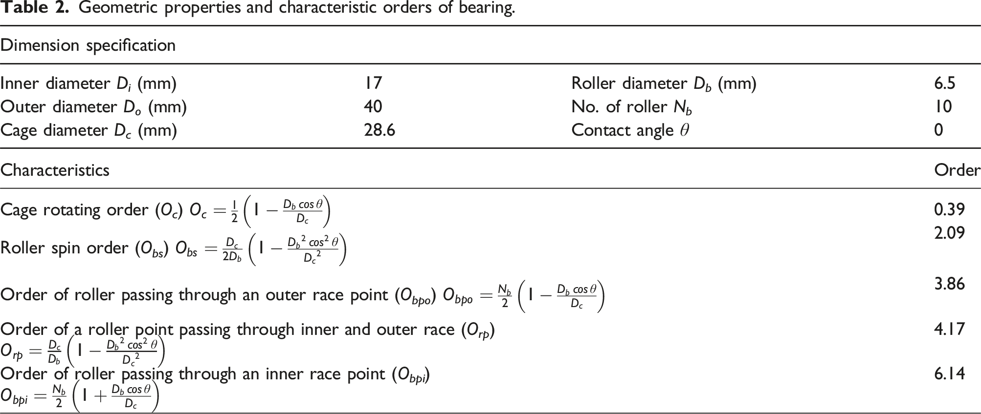
To assess the effectiveness and accuracy of the proposed diagnosis method, a bearing test rig was constructed to elucidate the operating conditions for defective bearings under varying rotation speed profiles. Figure 1 displays the images of the test rig and bearing defects along with the schematic plot. The test rig comprised a shaft supported by two sets of bearings (type: Koyo N203). To simulate operating conditions at varying speeds, the driving motor was set to four preset rotation speed profiles as follows (Figure 2): (A) constant speed, (B) speed-up and speed-down, (C) speed-down, and (D) speed-up. An accelerometer (PCB 352C33, U.S.A.) was affixed to the bearing support of the test rig to measure the resulting vibrations. A shaft encoder (Fotek MES-600, Taiwan) featuring 600 identical indices per revolution, was installed to obtain precise rotation speed measurements. Each index of the encoder generated a single pulse signal to trigger the data acquisition device (NI 9215, U.S.A.) which recorded vibration acceleration as an identical angular data series. The HOT technique can remove the influence of rotation speed variation and ensure that the characteristic orders of bearing defects (instead of the characteristic frequencies) are not governed by the rotation speed. The electrical discharge machining technique was used to create surface nicks of various sizes on the inner race, outer race, and roller of the bearings. One set of bearings in the test rig was replaced with a defective bearing to simulate the operating conditions involving various bearing defects. The experiment presented six test cases (Table 1), including a case that simulated normal conditions, as well as several cases with different types and levels of bearing defects. The experiment in this research mainly aimed to demonstrate the feasibility and effectiveness of using SAN to mitigate the interference caused by varying rotation speeds. Therefore, multiple-defect conditions, such as defects in different locations or on multiple elements of bearing, were not investigated for simplicity.

Figure 1.

(a) Image of the test rig; (b) Image of bearing defects; and (c) Schematic plot of test rig.

Figure 2.

Four preset profiles of rotation speed: (A) constant speed; (B) speed-up and speed-down; (C) speed-down; and (D) speed-up.

Table 1.

Illustrated six testing cases in this experiment.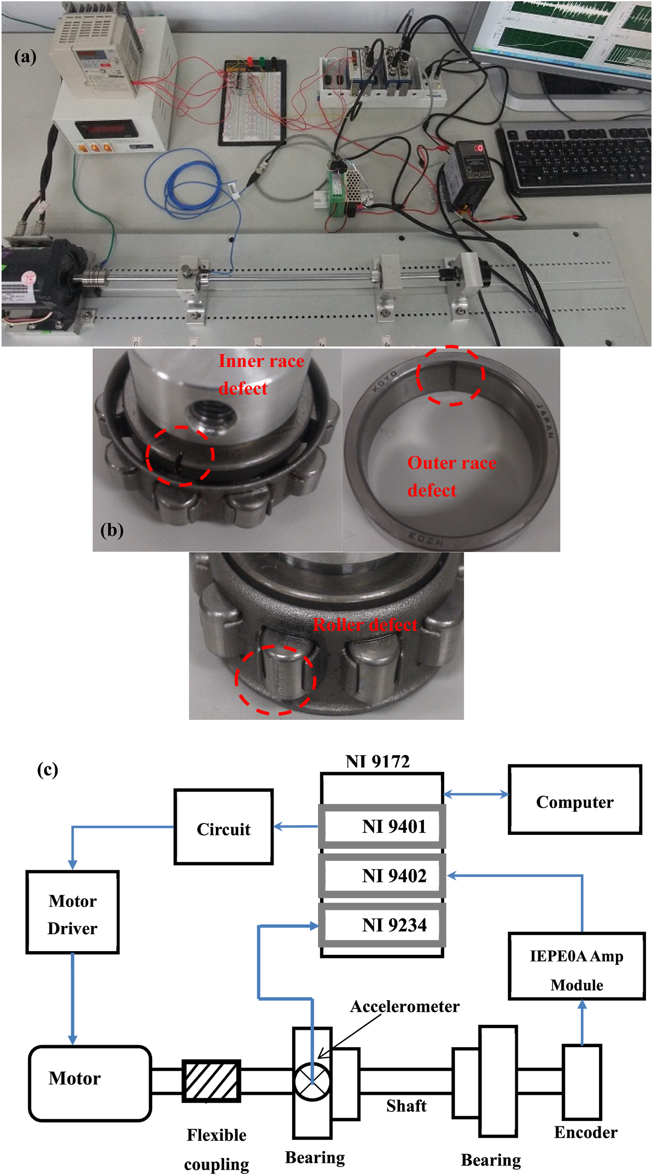

Case	Defect Expression	Nick dimension(mm)
Case 1	Normal
Case 2	Slight outer race defect	0.4 mm × 0.3 mm
Case 3	Severe outer race defect	0.8 mm × 0.3 mm
Case 4	Slight inner race defect	0.4 mm × 0.3 mm
Case 5	Severe inner race defect	0.8 mm × 0.3 mm
Case 6	Roller defect	0.1 mm × 0.3 mm

Each vibration signal data set was captured with identical angular increments and recorded continuously for 35 revolutions, resulting in a complete set of vibration signals comprising 21,000 data points. This measurement process was repeated 25 times for each shaft rotation speed profile. Each bearing defect test case encompassed 100 datasets of angle-domain vibration signals, leading to the acquisition of 600 sets of angle-domain vibration signals during the experiment. The signals were captured using LabVIEW software and processed on the MATLAB platform. All the measurement datasets are available on a cloud drive⁴¹ for further reference and application.

2.2 Vibration signal processing

The processing of vibration signals and extraction of features involved an analysis conducted in the angle and order domains. The envelope of vibration signals was first computed by employing the complex analytical signal method. Given that x(k) represents the measured vibration signal, the analytical signal z(k) can be calculated as follows:

z (k) = x (k) + j H [x (k)] = A (k) e^{j θ (k)},

(1)

where H[•] represents the Hilbert transform operator. The envelope can be calculated as follows:

A (k) = {(x {(k)}^{2} + H {[x (k)]}^{2})}^{1 / 2} .

(2)

Envelope signals are then decomposed into several intrinsic mode functions (IMFs) by applying the empirical mode decomposition (EMD) as follows:⁴²

A (k) = \sum_{i = 1}^{m} C_{i} (k) + r (k),

(3)

where C_i(k) represents the ith IMF and r(k) is the signal trend, which is a constant value or a monotonic curve. Each IMF exhibits a mono-oscillatory waveform and represents the signal component within a specific frequency band. The order (non-dimensional frequency) characteristics of bearing defects can be manifested in certain IMFs. Leveraging the geometric attributes of bearings, the characteristic orders of bearing can be determined (as outlined in Table 2). To examine the order range of individual IMFs, the instantaneous orders of IMFs were determined using the generalized zero-crossing (GZC) method.⁴³ This method stands as the foundational approach for computing local frequencies (orders) as it employs temporal control points to identify multiple categories of periods within a mono-oscillation component. With respect to the sample (time) intervals for zero-crossing, the following three classes of periods were considered.⁴³

Table 2.

Geometric properties and characteristic orders of bearing.

Dimension specification
Inner diameter D_i (mm)	17	Roller diameter D_b (mm)	6.5
Outer diameter D_o (mm)	40	No. of roller N_b	10
Cage diameter D_c (mm)	28.6	Contact angle θ	0
Characteristics			Order
Cage rotating order (O_c) $O_{c} = \frac{1}{2} (1 - \frac{D_{b} \cos θ}{D_{c}})$			0.39
Roller spin order (O_bs) $O_{b s} = \frac{D_{c}}{2 D_{b}} (1 - \frac{{D_{b}}^{2} \cos^{2} θ}{{D_{c}}^{2}})$			2.09
Order of roller passing through an outer race point (O_bpo) $O_{b p o} = \frac{N_{b}}{2} (1 - \frac{D_{b} \cos θ}{D_{c}})$			3.86
Order of a roller point passing through inner and outer race (O_rp) $O_{r p} = \frac{D_{c}}{D_{b}} (1 - \frac{{D_{b}}^{2} \cos^{2} θ}{{D_{c}}^{2}})$			4.17
Order of roller passing through an inner race point (O_bpi) $O_{b p i} = \frac{N_{b}}{2} (1 + \frac{D_{b} \cos θ}{D_{c}})$			6.14

(1) Whole period

The sample interval between two consecutive up (or down) zeros-crossings or two consecutive maxima (or minima) is counted as the period for this class. Each point along the angle axis has four values, which are determined on the basis of the period for this class.

(2) Half period

The sample interval from an up (or down) zero-crossing to the next down (or up) zero-crossing or that from a local maximum (or minimum) to the next local minimum (or maximum) is counted as the period for this class. Each point along the angle axis has two values, which are determined on the basis of the period for this class.

(3) Quarter period

The sample interval between a local extremum (maximum or minimum) and a zero-crossing is counted as the period for this class. Each point along the angle axis has only one value, which is determined on the basis of the period for this class.

The classes of whole, half, and quarter periods are designated as T_4j, T_2j, and T₁, respectively. Each point on the angle axis consists of seven (four for a full period, two for a half period, and one for a quarter period) values of periods. On the basis of the localness of the three classes of periods, the quarter period is determined to be the most local; thus, it has a weighting factor W₁ of 4. Because the half period is less local than the quarter period, it has a weighting factor W₂ of 2. Because the whole period is the least local of the three periods, it has the weighting factor W₄ of 1. The mean order of the ith IMF C_i(k) at each point along the angle axis can then be calculated as follows:

\bar{ω} (k) = \frac{W_{4} \sum_{i = 1}^{4} \frac{1}{T_{4 i}} + W_{2} \sum_{i = 1}^{2} \frac{1}{2 T_{2 i}} + W_{1} \frac{1}{4 T_{1}}}{4 W_{4} + 2 W_{2} + W_{1}} .

(4)

Vibration signal feature extraction

The features of vibration measurements are computed using angle-domain signals and order spectra. Once the envelope signals of vibration measurements are calculated and subsequently decomposed into various IMFs through the EMD method, the instantaneous orders for all IMFs are determined through GZC method, and the instantaneous magnitude of the corresponding IMF is calculated. As a result, the extracted features comprise both angle-domain and order-domain characteristics. Within each domain, these features are categorized into two groups, each encompassing the respective orders (as indicated in Table 4). The procedure of feature extraction is outlined and illustrated as follows:

(1) Angle-domain feature of the first group

The IMFs whose orders comprise the characteristic orders (Table 2) were extracted. The selected IMF is denoted as the series X = [x₁, x₂,…, x_N], and the root-mean-square (RMS) value of X is obtained as the angle-domain feature of the first group:

X_{r m s} = \sqrt{\frac{1}{N} \sum_{i = 1}^{N} x_{i}^{2}} .

(5)

(2) Angle-domain feature of the second group

Utilizing the computed instantaneous order and amplitude, the angle-order spectrum is formulated as H(θ, o), and the marginal order spectrum h(o) can be obtained by integrating H(θ, o) along the angle axis (θ). Let the order spectral amplitude at the jth characteristic order be expressed as h(o_j). The RMS value of the jth characteristic order in an individual IMF is defined as follows:

o_{r m s, j} = X_{r m s} \frac{h (o_{j})}{M},

(6)

where M represents the total amplitude of an order spectrum and is defined as follows:

M = \int_{o} h (o) d o .

(7)

The RMS value of the jth characteristic order within the Q IMFs is then extracted as the angle-domain feature of the second group and defined as follows:

O_{r m s, j} = \sum_{q = 1}^{Q} {(o_{r m s, j})}_{q} .

(8)

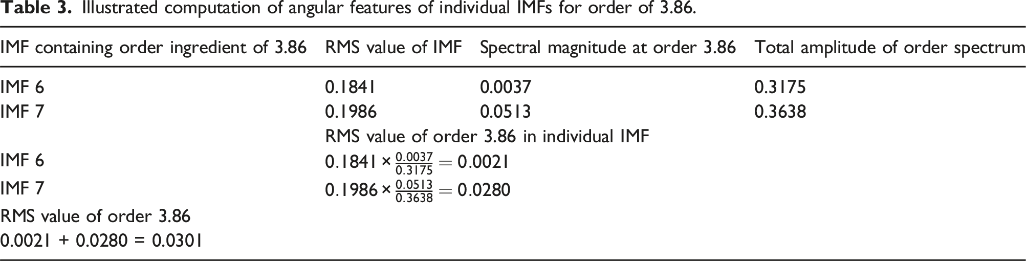
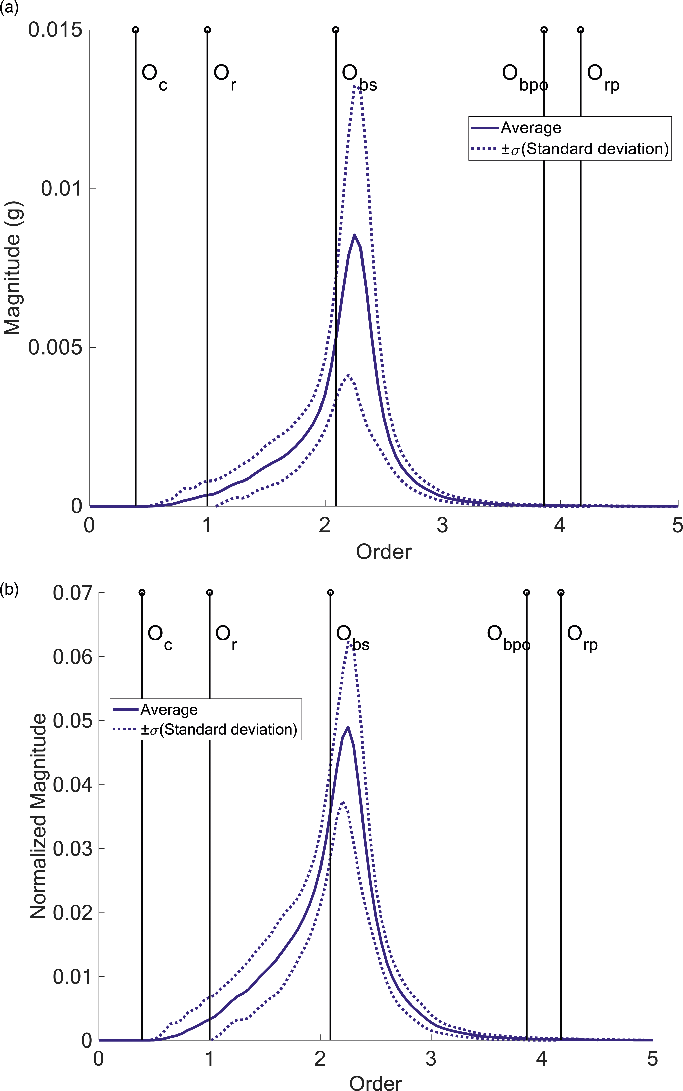
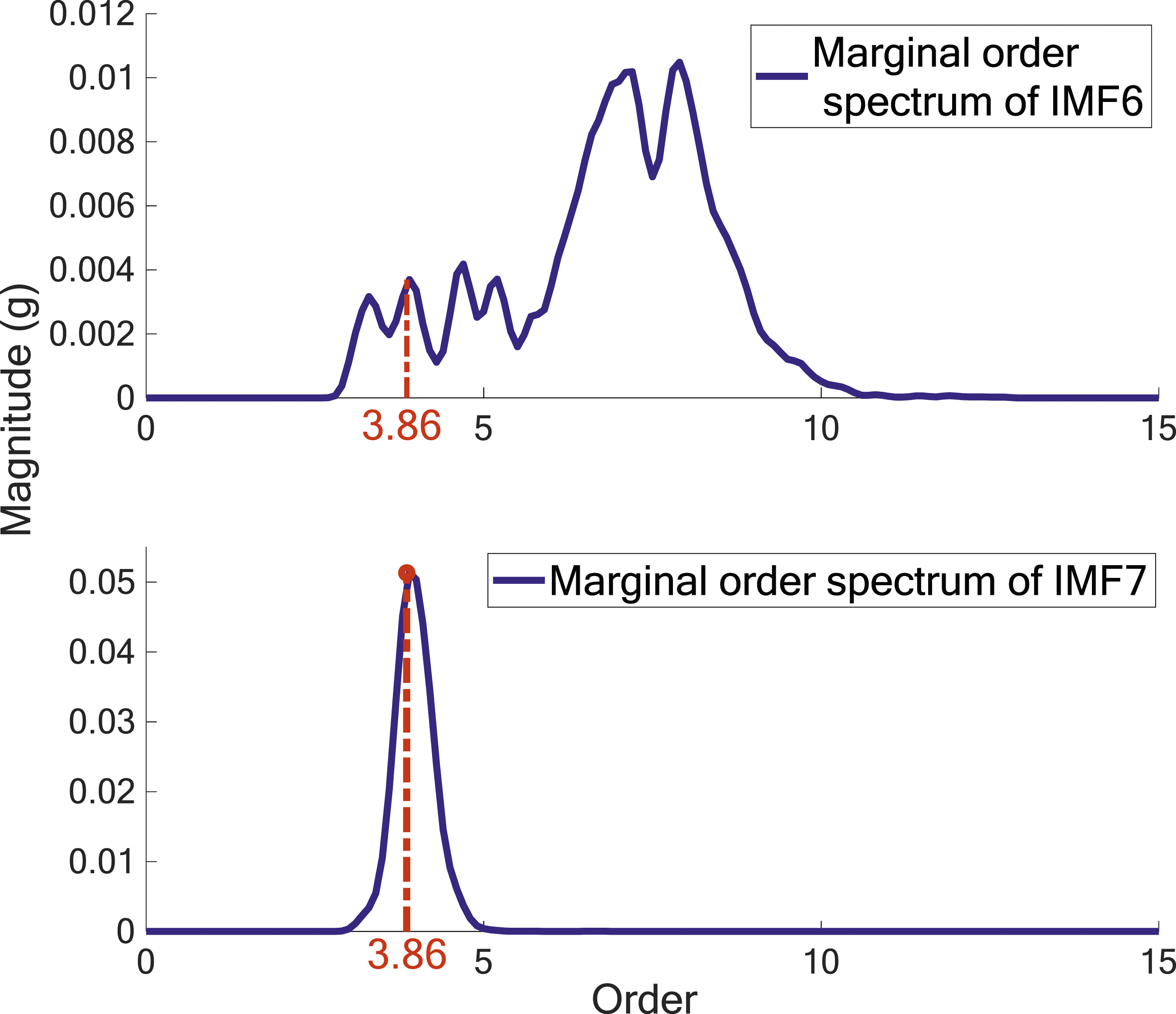
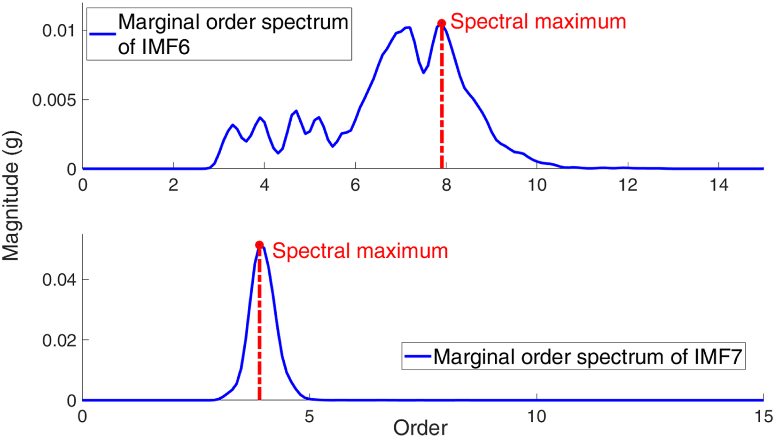
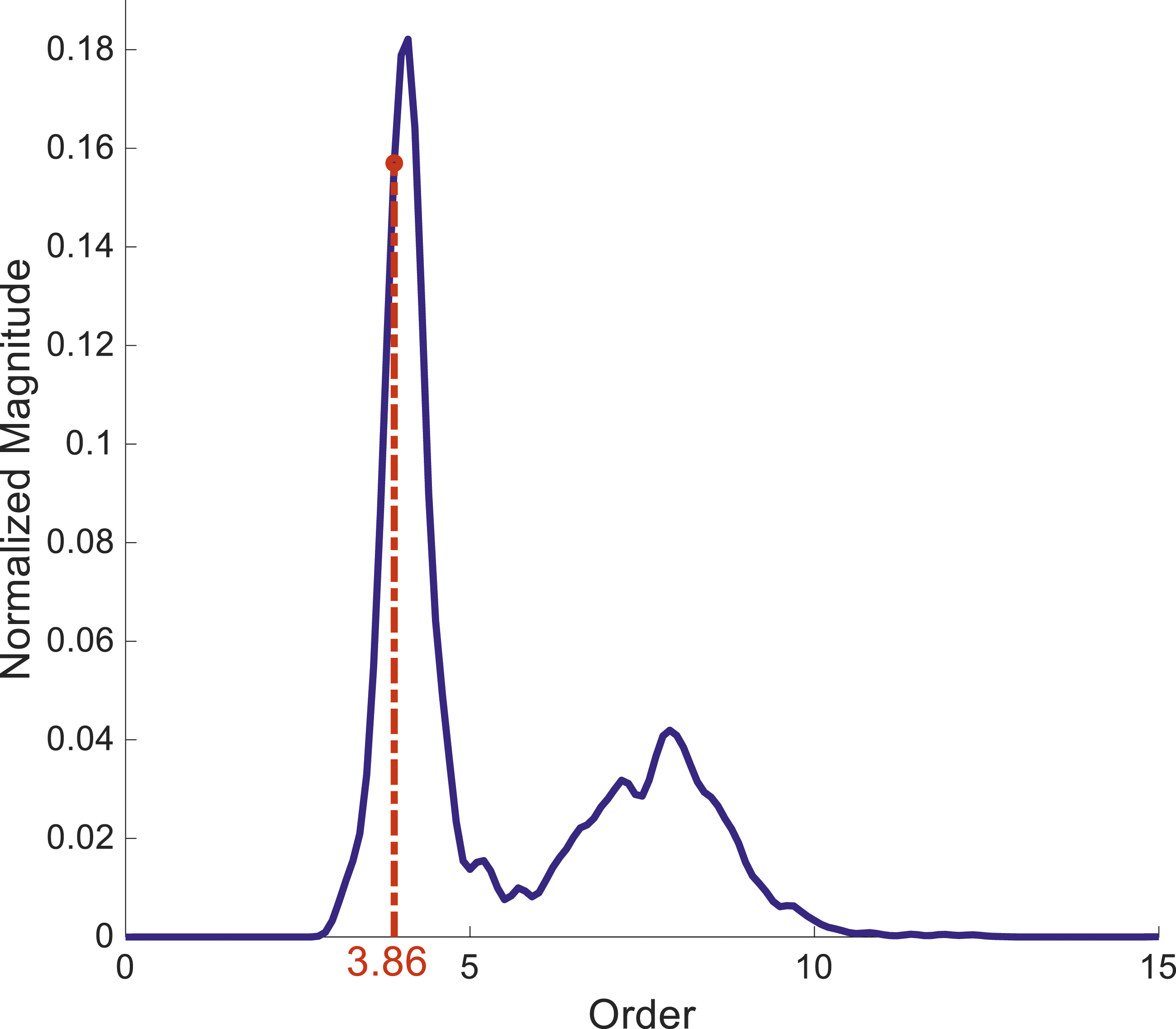
The angular feature of the order corresponding to rollers passing through an outer race point (O_bpo = 3.86) is depicted in Figure 3. This highlights IMFs 6 and 7 of the envelope signal, both of which contain the order component of 3.86. This observation was made in the case with rotation speed profile D (Figure 2(d)). The corresponding marginal order spectra are presented in Figure 4. Subsequently, the computation of angular features for each individual IMF is tabulated (Table 3) in relation to the order of 3.86.

Figure 3.

IMFs 6 and 7 of envelope signal containing order ingredient of 3.86 with rotation speed profile D.

Figure 4.

Marginal order spectra of IMFs 6 and 7.

Table 3.

Illustrated computation of angular features of individual IMFs for order of 3.86.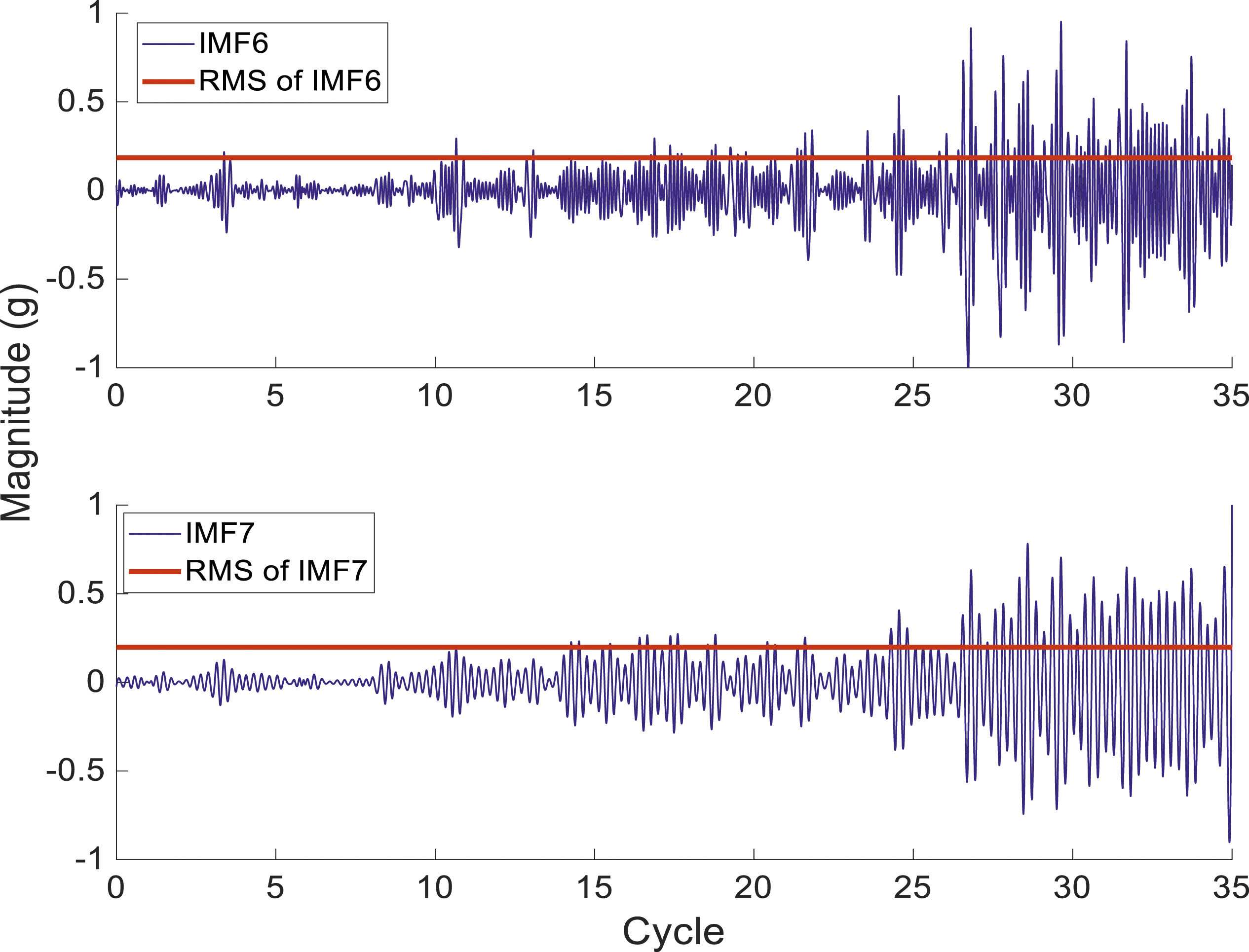

IMF containing order ingredient of 3.86	RMS value of IMF	Spectral magnitude at order 3.86	Total amplitude of order spectrum
IMF 6	0.1841	0.0037	0.3175
IMF 7	0.1986	0.0513	0.3638
	RMS value of order 3.86 in individual IMF
IMF 6	$0.1841 \times \frac{0.0037}{0.3175} = 0.0021$
IMF 7	$0.1986 \times \frac{0.0513}{0.3638} = 0.0280$
RMS value of order 3.86
0.0021 + 0.0280 = 0.0301

Order-domain features are selected from the marginal order spectrum, and the following quantitative process is applied for order-domain features.

(3) Order-domain feature of the first group

The spectral magnitude of the specific IMFs at the jth characteristic order, h(o_j), is extracted as the order-domain feature of the first group.

(4) Order-domain feature of the second group

The spectral maximum magnitude h_max (o) of the IMFs containing the jth characteristic order is selected as the order-domain feature of the second group.

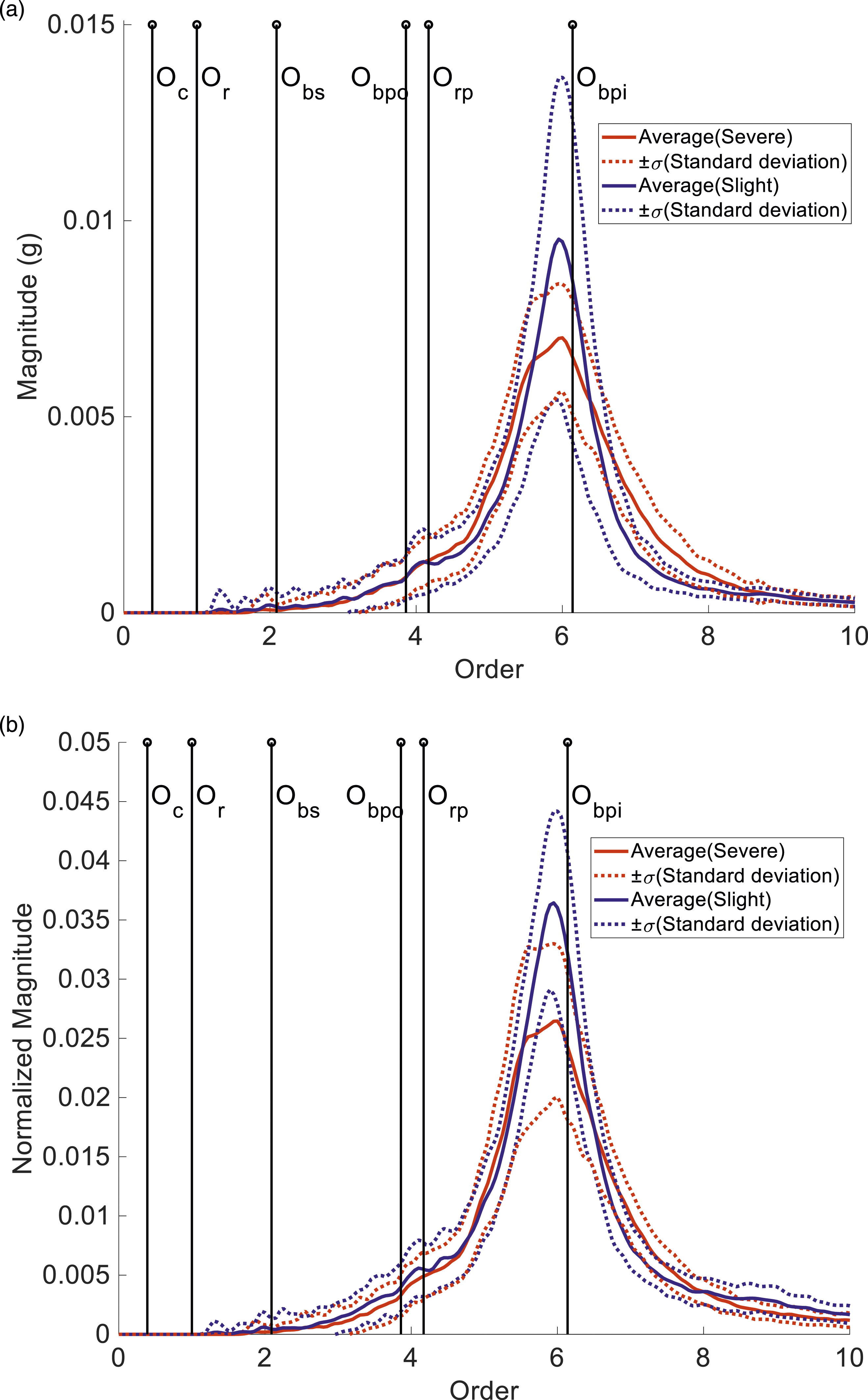
The calculation process of the order features related to 3.86 (O_bpo, the order of rollers passing through an outer race point) is carried out as follows. Since IMFs 6 and 7 encompass the order of 3.86, the associated marginal order spectrum is constructed by integrating the angle-order distribution along the θ axis, in which IMFs 6 and 7 are both included. Figure 5 displays the plot of the marginal order spectrum for the synthesized signal (including IMFs 6 and 7). The spectral magnitude at the order of 3.86 is extracted as the order-domain features of the first group. The order-domain features of the second group are selected from the spectral maximum magnitude of IMFs 6 and 7, both of which contain the characteristic order of 3.86 (as depicted in Figure 6).

Figure 5.

Marginal order spectrum of synthesized signal (IMFs 6 and 7).

Figure 6.

Order-domain features of the second group: spectral maximum magnitude of the IMFs 6 and 7 that contain order of 3.86.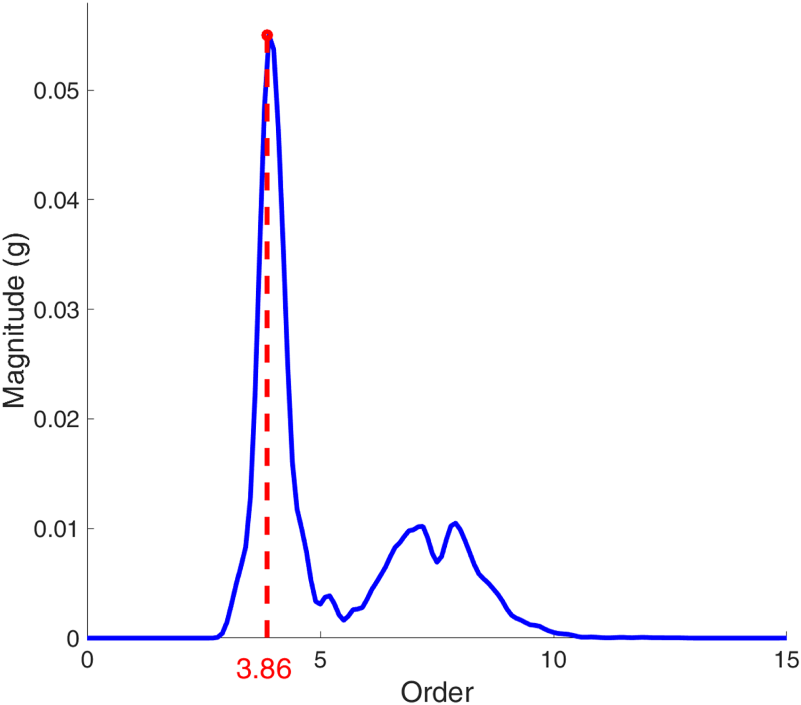

SAN

The HOT technique can normalize the characteristic frequencies of bearings in terms of the orders in cases involving varying rotation speeds. As a result, the frequency-domain features related to bearing flaws can be extracted as fixed order values. However, varying rotation speeds inevitably lead to variations in vibration energy. Generally, vibration energy also fluctuates depending on the level of bearing defect during the bearing’s deterioration. The causes of vibration energy variation that are attributed to the two aforementioned phenomena may be coupled with each other. In such situations, the diagnosis of bearing deterioration is affected by interference. Therefore, the proposed SAN scheme is employed to enable the extraction of normalized and consistent features.

(1) Extraction of angle-domain feature of the first group through SAN

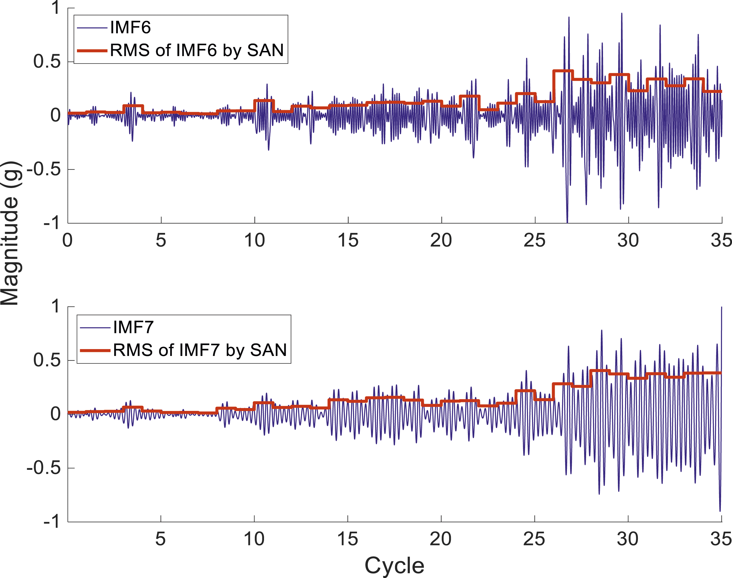
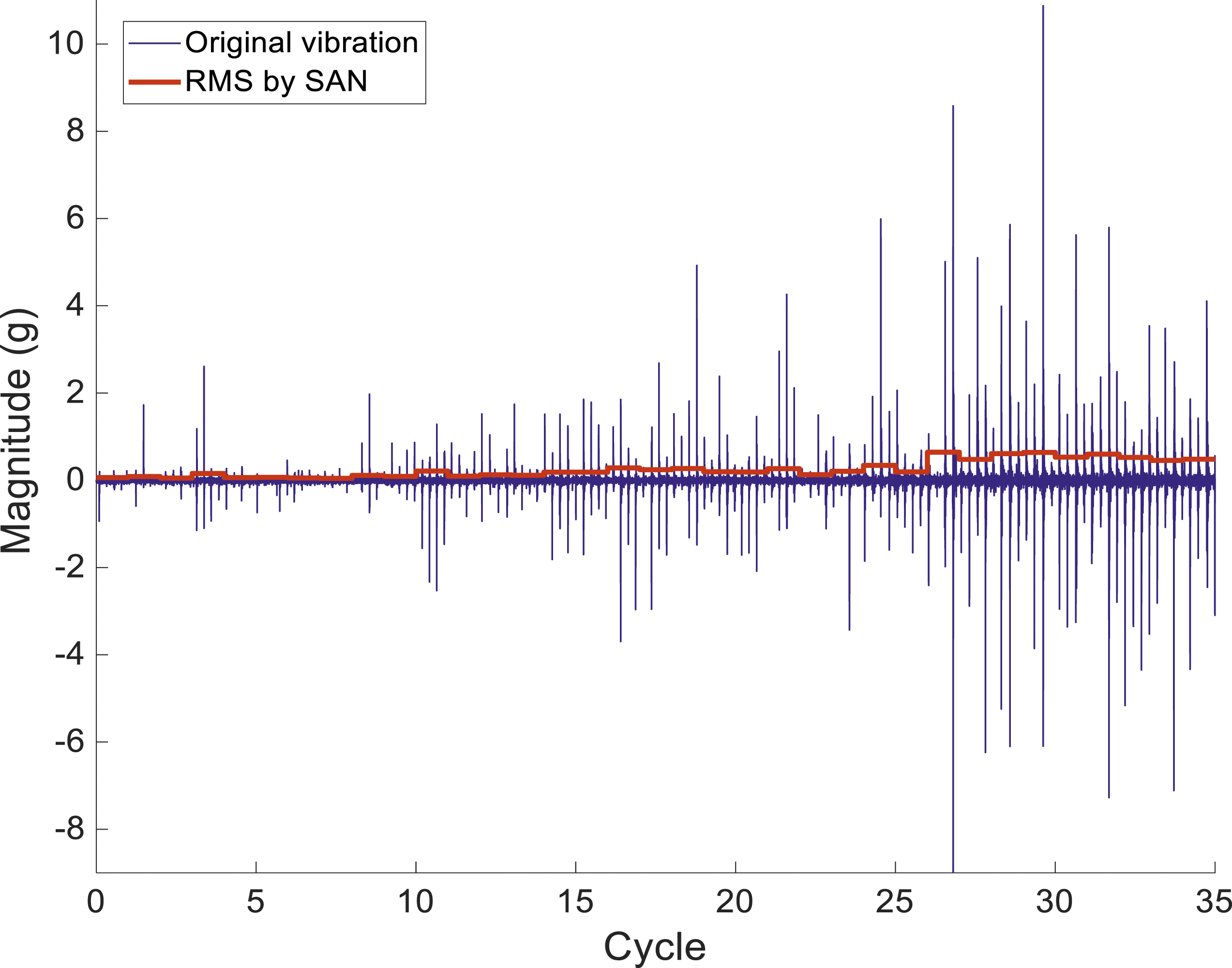
The angle-domain features of the first group, namely, the RMS values of the selected IMFs, undergo modification through SAN. In other words, the RMS values of the selected IMFs are calculated independently for each cycle. Figures 7–9 illustrate the application of SAN to obtain the RMS values of IMFs 6 and 7, which encompass the order of 3.86. In Figure 7, the red lines depict the RMS values of the IMFs (represented by blue lines) for each cycle. The RMS values of the original vibration signal are also computed for each cycle (as shown in Figure 8). Subsequently, the RMS values of the IMFs within an individual cycle are divided by the RMS values of the original vibration signal from the corresponding cycles. This division yields normalized RMS values (depicted by blue line in Figure 9). Consequently, the mean value of the normalized RMS values of a selected IMF encapsulates the angle-domain features of the first group, as attained through SAN.

(2) Extraction of angle-domain feature of the second group through SAN

Figure 7.

RMS values of IMFs 6 and 7 with SAN.

Figure 8.

RMS values of original vibration signal.

Figure 9.

Normalized RMS values of IMFs 6 and 7.

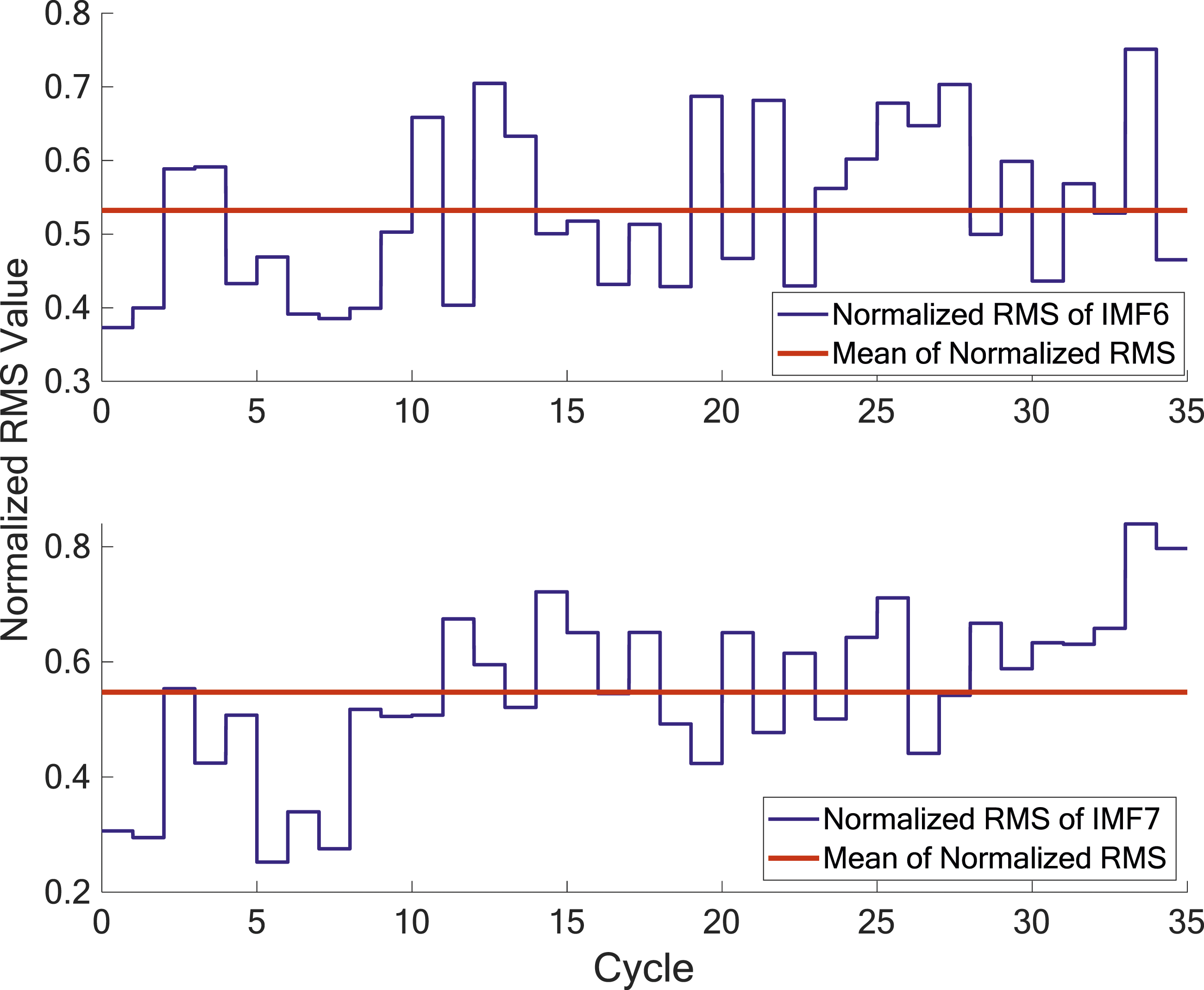
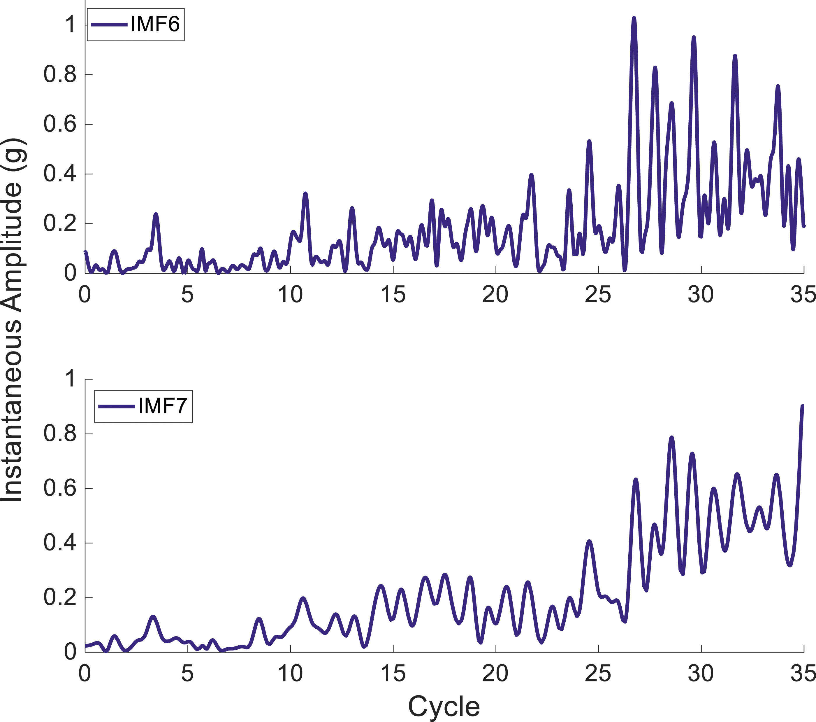
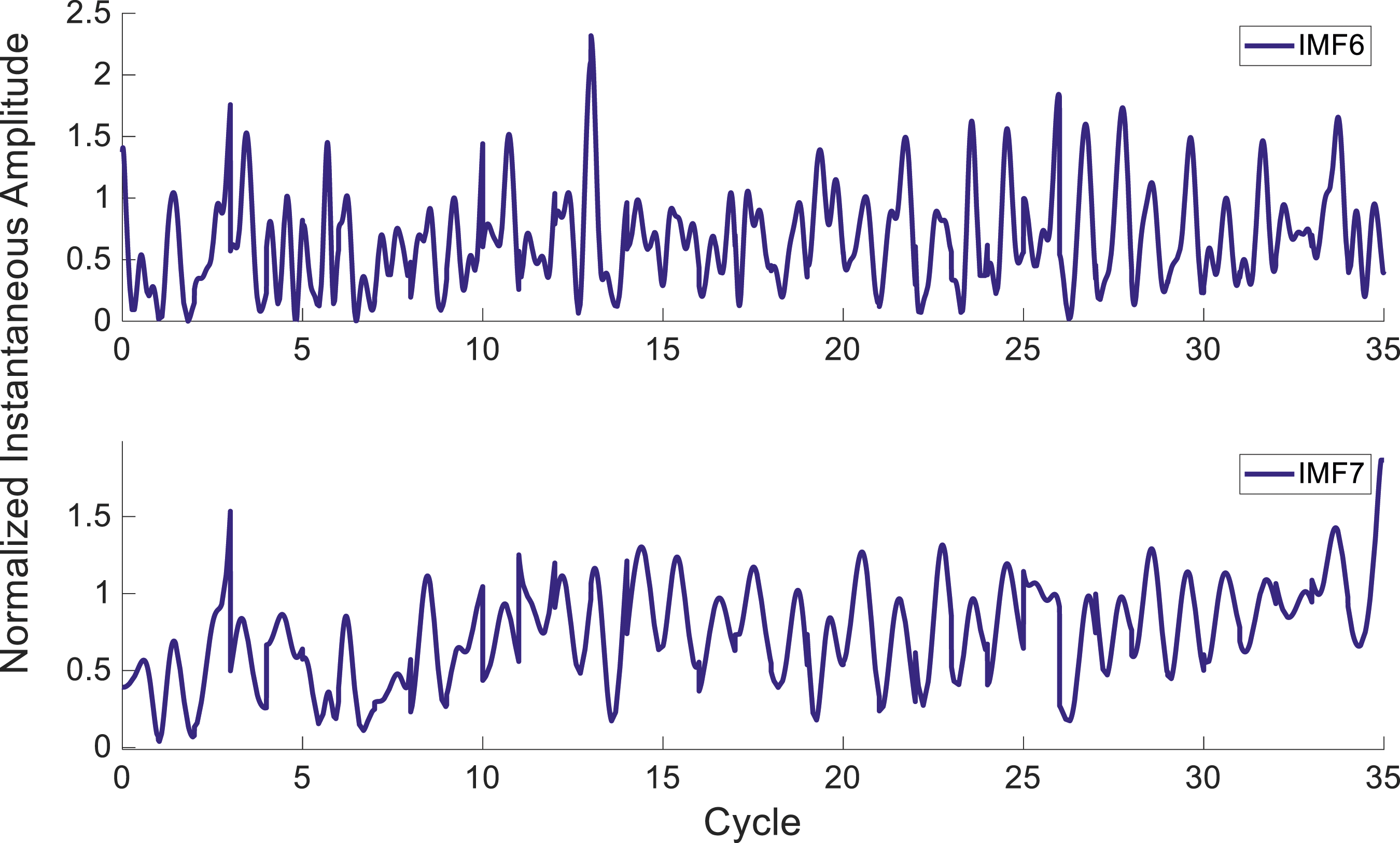
The instantaneous amplitude of the selected IMFs are calculated (as depicted in Figure 10). Figure 10 illustrates a graph displaying the instantaneous amplitudes of IMFs 6 and 7 (order of 3.86). Subsequently, these amplitudes are divided by the cyclical RMS values of the original signal (shown as the red line in Figure 8), resulting in normalized instantaneous amplitudes (as shown in Figure 11). These examples suggest that the variation in instantaneous amplitude caused by varying rotation speeds can be mitigated. The normalized marginal order spectra of IMFs 6 and 7 are then generated using the normalized instantaneous amplitude of the corresponding IMFs. The angle-domain feature of the second group (as obtained through SAN) can be ascertained following the steps outlined in Figures 3 and 4 as well as Table 3.

(3) Extraction of order-domain feature of the first group through SAN

Figure 10.

Instantaneous amplitude of IMFs 6 and 7.

Figure 11.

Normalized instantaneous amplitude of IMFs 6 and 7.

Using SAN, the normalized spectral magnitude of the IMFs at the jth characteristic order, denoted as h(o_j), is acquired as the order-domain feature of the first group. Figure 12 illustrates the normalized marginal order spectrum of the synthesis of IMFs 6 and 7, both of which possess the characteristic order of 3.86. The magnitude of O_bpo (order of 3.86) is then extracted as an order-domain feature of the first group.

(4) Extraction of order-domain feature of the second group through SAN

Figure 12.

Normalized marginal order spectrum of synthesis of IMFs 6 and 7 containing order of 3.86.

Using SAN, the maximum magnitude of the normalized marginal order spectrum linked to the IMF containing the jth characteristic order is selected as the order-domain feature of the second group. Figure 13 depicts the normalized marginal order spectra of IMFs 6 and 7, both of which hold the characteristic order of 3.86. The highest value of the normalized marginal order spectrum’s peak is then extracted as an order-domain feature of the second group.

Figure 13.

Normalized marginal order spectra of IMFs 6 and 7 (containing order of 3.86) and corresponding peaks values.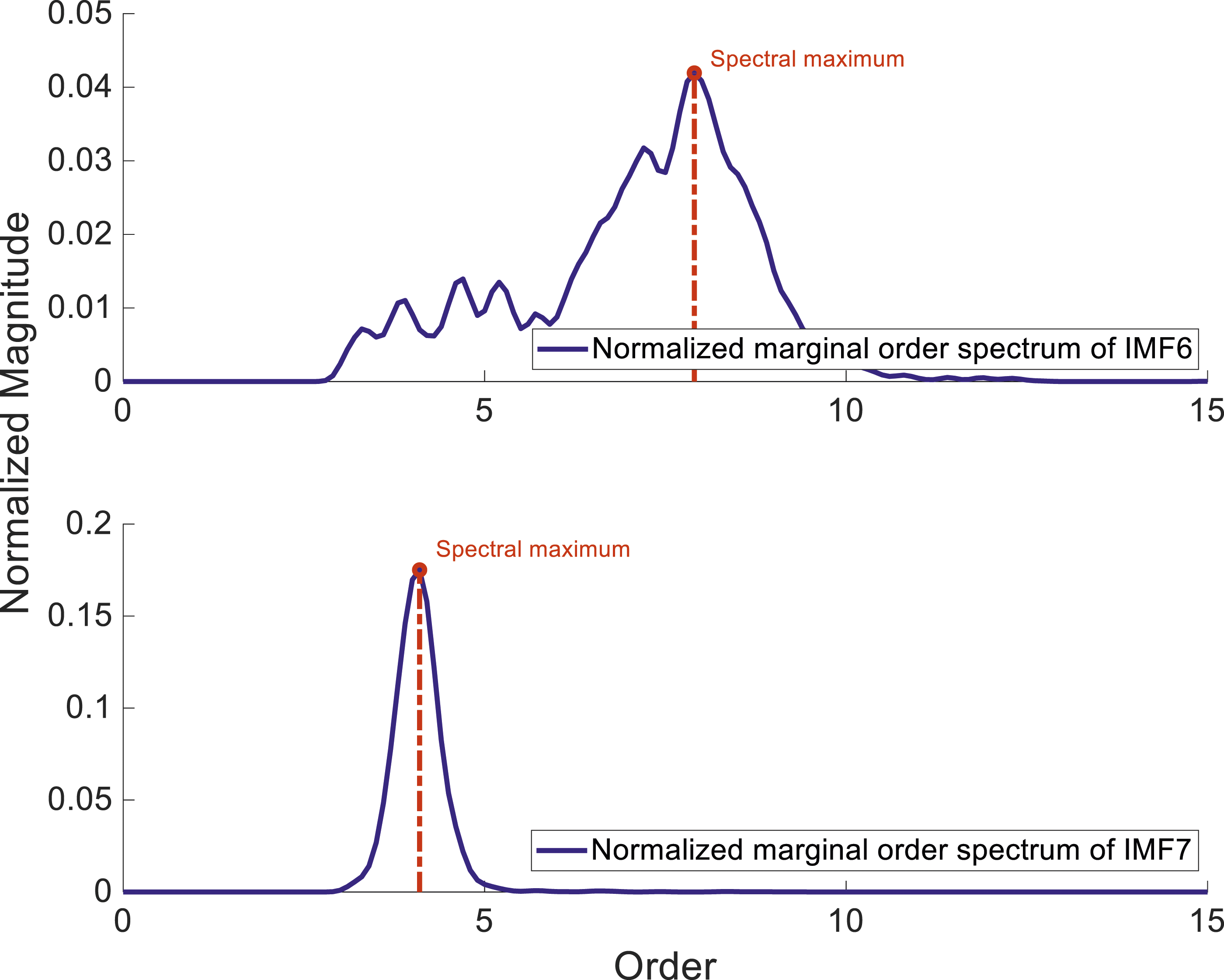

Signal feature analysis and experimental verification

The vibration measurements from the six cases (as listed in Table 1) were collected and analyzed. The envelope of the vibration signals was computed and subsequently decomposed into several IMFs using EMD. The instantaneous orders of IMFs were calculated, allowing for the identification and selection of IMF components that correspond to the characteristic orders outlined in Table 2. The selected IMFs, along with their associated instantaneous orders that encompass characteristic orders, are presented in Table 4.

Table 4.

Selected IMFs with instantaneous orders that comprise characteristic orders.

IMF	Corresponding characteristic order
IMF6	O _bpi
IMF7	O _rp ,O _bpo
IMF8	O _bs
IMF9	O _r
IMF10	O _c
IMF11	O _c

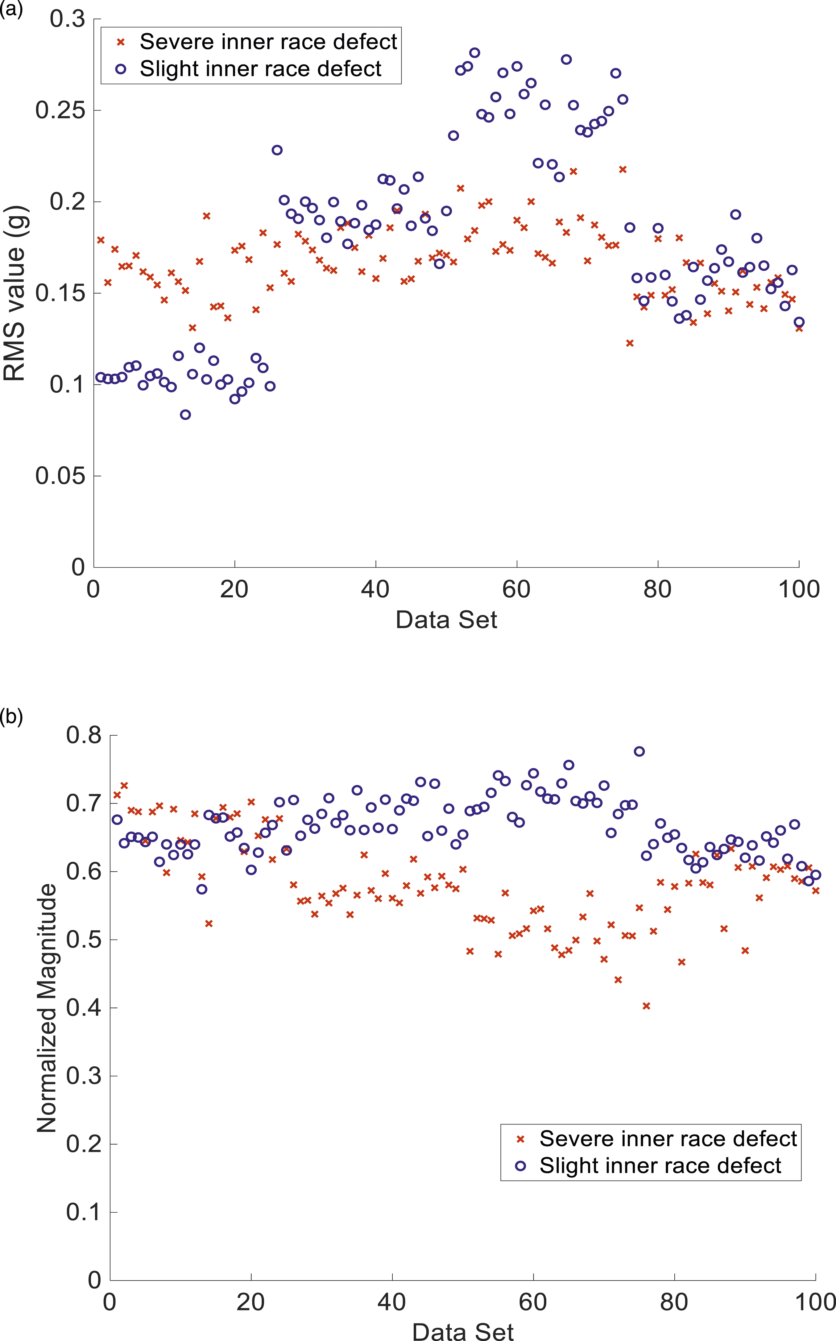
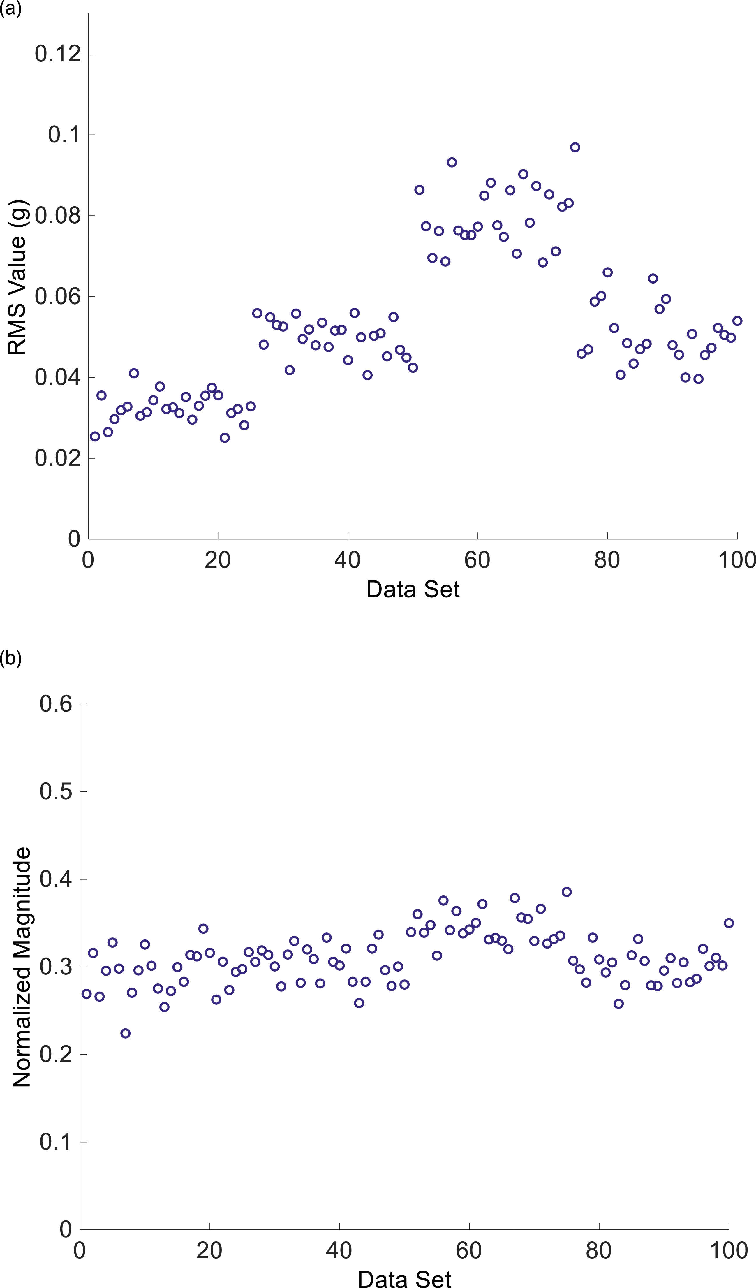
To validate the efficacy of SAN for mitigating vibration energy fluctuations attributed to varying rotation speeds, the selected features of defective bearings were obtained through both direct calculation and the employment of SAN. Subsequently, a comparison was conducted between the outcomes obtained via these two approaches. Figures 14–19 illustrate the results of this comparison for several extracted features. In the provided data representation, numbers 1–25 pertain to the features of signals collected under rotation speed profile A, while numbers 26–50, 51–75, and 76–100 correspond to features from signals collected under rotation speed profile B, C, and D, respectively.

Figure 14.

(a) RMS values of IMF 7 for experimental cases 2 (slight outer race defect, blue circles) and 3 (severe outer race defect, red cross) without SAN (b)Normalized RMS values of the IMF 7 for experimental cases 2 (slight outer race defect, blue circles) and 3 (severe outer race defect, red cross) through SAN.

Figure 15.

(a) Marginal order spectrum of IMF 7 without SAN process; blue: slight outer race defect; red: severe outer race defect; solid: mean value of all data sets; dotted: ± σ (standard deviation) of data sets based on their average value (b) Normalized marginal order spectrum of IMF 7 with SAN process; blue: slight outer race defect; red: severe outer race defect; solid: mean value of all data sets; dotted: ± σ (standard deviation) of data sets based on their average value.

Figure 16.

(a) RMS values of IMF 6 in experimental cases 4 (slight inner race defect, blue circles) and 5 (severe inner race defect, red cross) without SAN (b) Normalized RMS values of IMF 6 in experimental cases 4 (slight inner race defect, blue circles) and 5 (severe inner race defect, red cross) with SAN.

Figure 17.

(a) Marginal order spectrum of IMF 6 without SAN process; blue: slight inner race defect; red: severe inner race defect; solid: mean value of data sets; dotted: ± σ (standard deviation) of data sets based on their average value (b) Normalized marginal order spectrum of IMF 6 with SAN process; blue: slight inner race defect; red: severe inner race defect; solid: mean value of data sets; dotted: ± σ (standard deviation) of data sets based on their average value.

Figure 18.

(a) RMS values of IMF 8 in experimental case 6 (roller defect) without SAN. (b) Normalized RMS values of IMF 8 in experimental case 6 (roller defect) with SAN.

Figure 19.

(a) Marginal order spectrum of IMF 8 without SAN; solid: mean value of data sets; dotted: ± σ (standard deviation) of data sets based on their average value (b) Normalized marginal order spectrum of IMF 8 with SAN; solid: mean value of data sets; dotted: ± σ (standard deviation) of data sets based on their average value.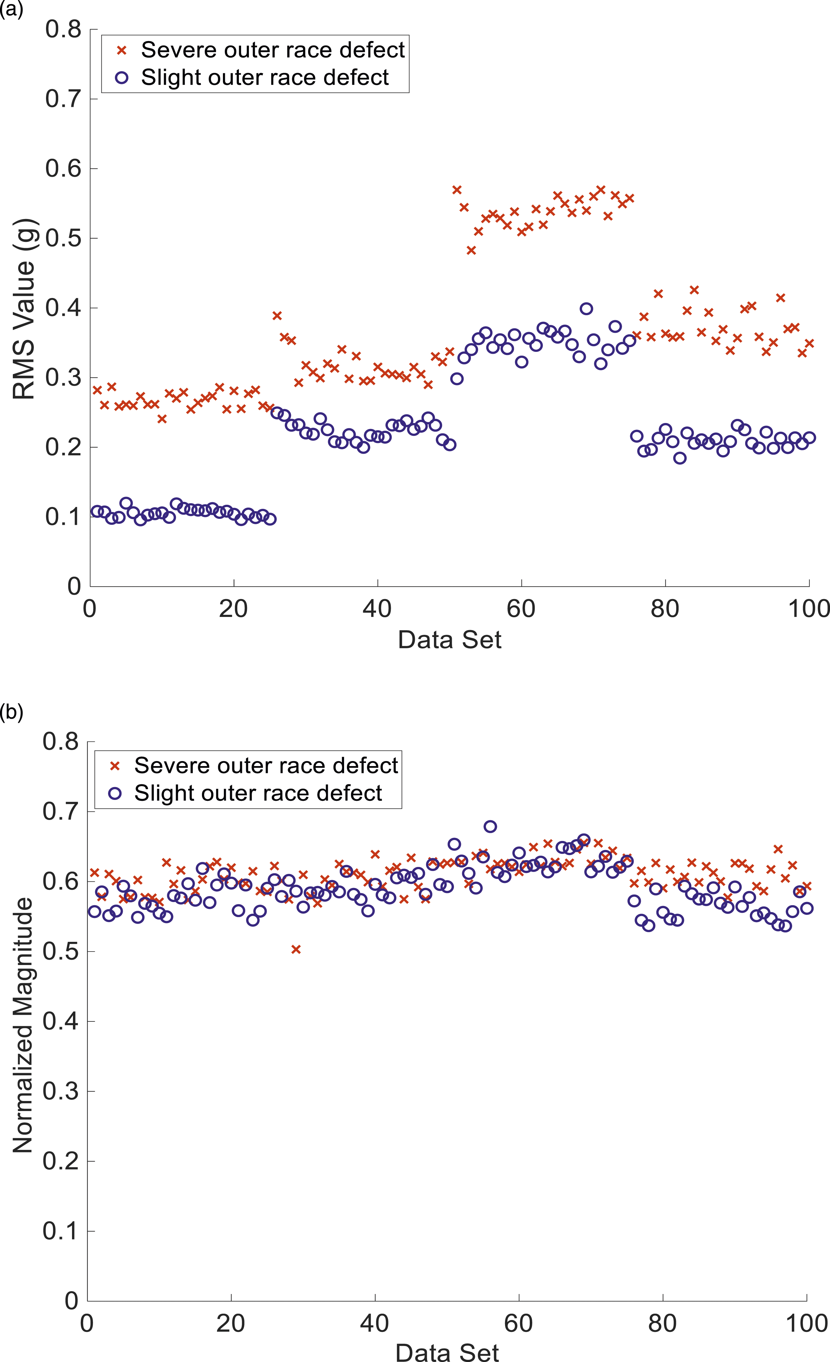

Outer race defect

A significant characteristic related to an outer race defect primarily concerns the order of the roller passing through a point on the outer race, termed O_bpo, which resides within IMF 7. Illustrated in Figure 14 are the RMS values of IMF 7 (denoting angle-domain features) for experimental cases 2 (slight outer race defect as depicted by blue circles) and 3 (severe outer race defect as indicated by red crosses). One dataset was acquired without employing SAN as shown in Figure 14(a), while the other was obtained by using SAN as presented in Figure 14(b). Figure 14(a) reveals that IMF 7 exhibited various RMS values for different data numbers (owing to varying rotation speeds) when the features were not subjected to SAN processing. In contrast, Figure 14(b) showcases that the normalized RMS values of IMF 7 were adjusted to maintain consistency even in the presence of vibration energy variations resulting from varying rotation speeds. Namely, SAN is capable of reducing the feature variation caused by different rotation speed profiles, which is beneficial for diagnosing various bearing defects under varying shaft rotation speeds.

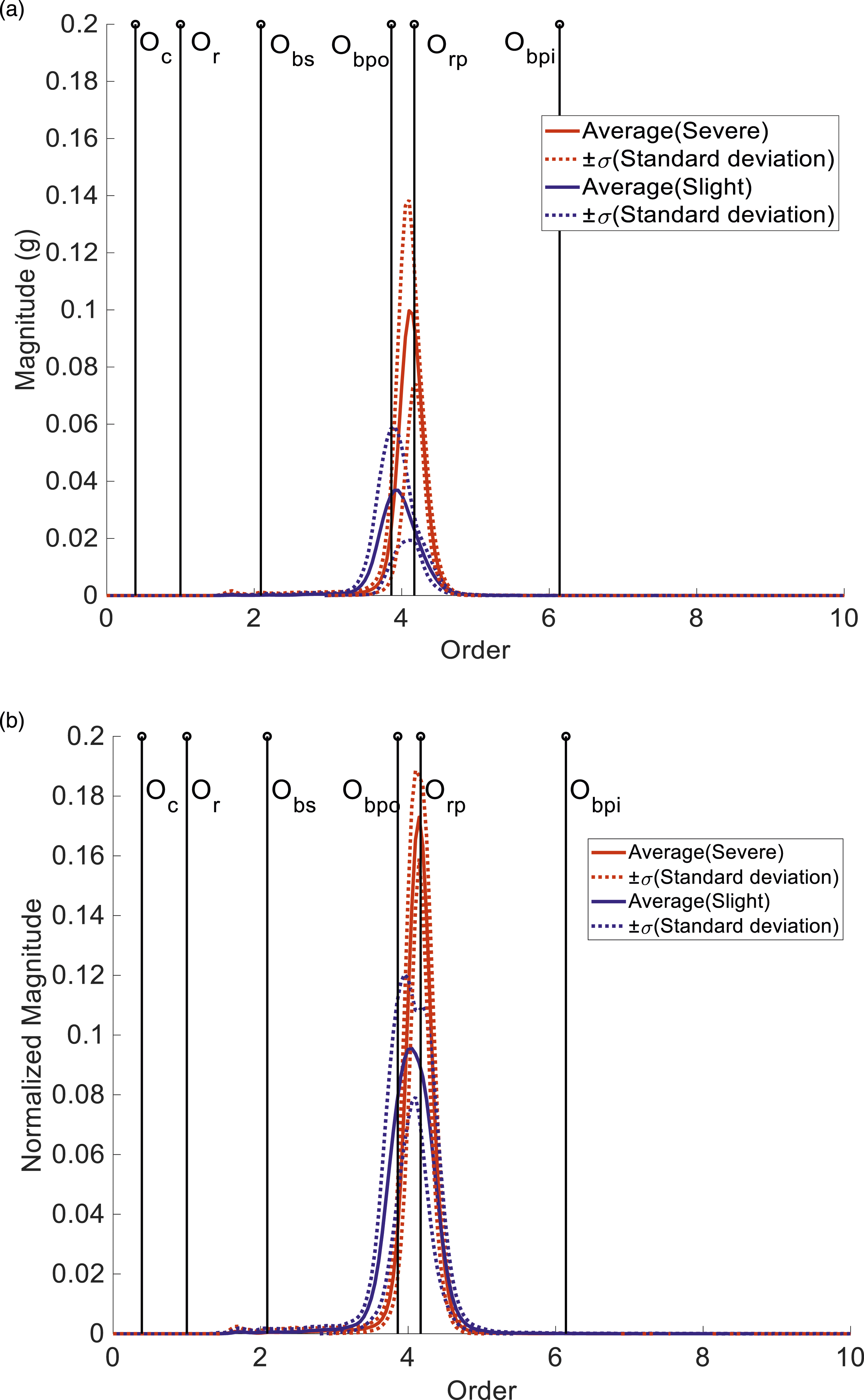
Figure 15 unveils the characteristics within the marginal order spectrum of IMF 7, which signifies order-domain features. Two sets of data are presented: one acquired without employing SAN (Figure 15(a)), and the other obtained using SAN (Figure 15(b)). The solid lines, blue indicating slight outer race defect and red indicating severe outer race defect, illustrate the mean values of the order spectrum across the 100 data sets. Accompanying these solid lines are dotted lines depicting the range of ± σ (standard deviation) from their average values for the 100 data sets. Significantly, in the absence of SAN application, substantial differences were evident between the average values (solid lines) and ± σ ranges (dotted lines) due to the influence of varying rotation speeds (Figure 15(a)). However, with the utilization of SAN, the discrepancies between the solid and dotted lines were significantly reduced (shown in Figure 15(b)). This observation suggests that SAN possesses the capability to diminish the deviations within order spectra. Specifically, the normalized order spectral magnitude displayed a tendency toward consistency and concentration, despite the presence of varying rotation speeds that led to fluctuations in vibration energy. This mitigation of vibration energy fluctuation holds values for diagnosing multiple levels of bearing defects in scenarios involving varying rotation speeds.

Inner race defect

Similar observations were made regarding the analysis of the selected feature for cases involving slight and severe inner race defects (experimental cases 4 and 5). A significant characteristic of inner race defects relates primarily to the order of the roller passing through an inner race point (O_bpi) which is contained in IMF 6. The results for the analysis of angle-domain features are presented in Figure 16. This figure depicts the RMS values of IMF 6 in experimental cases 4 (indicated by blue circles, representing slight inner race defect) and 5 (indicated by red crosses, representing severe inner race defect). One set of data was obtained without employing SAN (Figure 16(a)), while the other was obtained by applying SAN (Figure 16(b)). Figure 16(a) reveals that without SAN, the RMS values of the data sets could be categorized into four groups, attributed to the variation in vibration energy due to the four rotation speed profiles. Similar outcomes were obtained for the cases involving slight and severe outer race defects (Figure 14). When SAN was applied, the consistency of the normalized RMS magnitude of all the data sets was improved (Figure 16(b)).

Similar observations were made in relation to the analysis of order-domain features. Figure 17 presents the marginal order spectra of IMF 6 as obtained without employing SAN (Figure 17(a)) and with the application of SAN (Figure 17(b)). The cases involving slight and severe inner race defects (cases 4 and 5) are indicated by blue and red lines, respectively. The solid lines represent the average order spectrum value of 100 data sets, while the dotted lines represent the range of ± σ (standard deviation) from their average values for the 100 data sets. As shown in Figure 17(a) and (b), the discrepancy between the average values (solid lines) and ± σ (dotted lines) was decreased with employing SAN. This change was particularly pronounced for slight inner race defects (blue lines), indicating that the order spectral magnitude was normalized. This normalization led to consistency and concentration across multiple data sets corresponding to varying rotation speeds. Consequently, SAN proves to be beneficial for diagnosing various levels of bearing defects at varying rotation speeds.

Roller defect

A significant aspect related to roller defects primarily concerns the order of roller spin (O_bs), which is encapsulated in IMF 8. The outcomes of the analysis of angle-domain features are displayed in Figure 18. This figure illustrates the RMS values of IMF 8 in experimental Case 6 (roller defect). One dataset was acquired without employing SAN (Figure 18(a)), while the other was acquired with the application of SAN (Figure 18(b)). In the absence of SAN, distinct and discernible clusters of RMS values were evident among the data sets (Figure 18(a)). Upon implementing SAN (Figure 18(b)), the normalized magnitude indicated an enhanced consistency of the RMS values across the data sets. Consequently, SAN mitigated the impact of vibration energy fluctuations resulting from varying rotation speeds.

The findings pertaining to the analysis of order-domain features are showcased in Figure 19, depicting the marginal order spectra of IMF 8 obtained without employing SAN (Figure 19(a)) and with the application of SAN (Figure 19(b)). A comparison between the outcomes in Figure 19(a) and (b) reveal that the disparities between the average value (solid line) and ± σ (dotted lines) were diminished through SAN. This discovery implies that the characteristics of roller defects in the order domain can be normalized, maintaining consistency even in the face of vibration energy variation arising from varying rotation speeds. Consequently, SAN enhances the uniformity of bearing defect features among datasets in scenarios involving varying rotation speeds, proving beneficial for the diagnosis of multiple types and levels of bearing defects.

Diagnosis results and discussion

To validate the efficacy of the proposed SAN method in diagnosing bearing defects at varying rotation speeds and highlight the enhancements achieved by its implementation, a SVM ^44,45 was employed as the machine learning approach to classify different classes and levels of bearing defects. The computed extracted features (as described in subsections 2.3 and 2.4) encompassed the following angle-domain and order-domain features:

(1) RMS values of IMFs 6–11 (constituting the angle-domain feature of the first group).

(2) RMS values of orders 0.39, 1, 2.09, 3.86, 4.17, and 6.14 (forming the angle-domain feature of the second group).

(3) Magnitude of the order spectra at orders 0.39, 1, 2.09, 3.86, 4.17, and 6.14 (comprising the order-domain feature of the first group).

(4) Peak values of the order spectra for IMFs 6–11 (comprising the order-domain feature of the second group).

Subsequently, the proposed SAN method was applied to the feature groups (1), (2), (3), and (4) to obtain the normalized feature groups (5), (6), (7), and (8), respectively. The entire bearing defect diagnosis process using the proposed approach is organized as shown in the flowchart in Figure 20.

Figure 20.

Flowchart of bearing defect diagnosis through the proposed approach.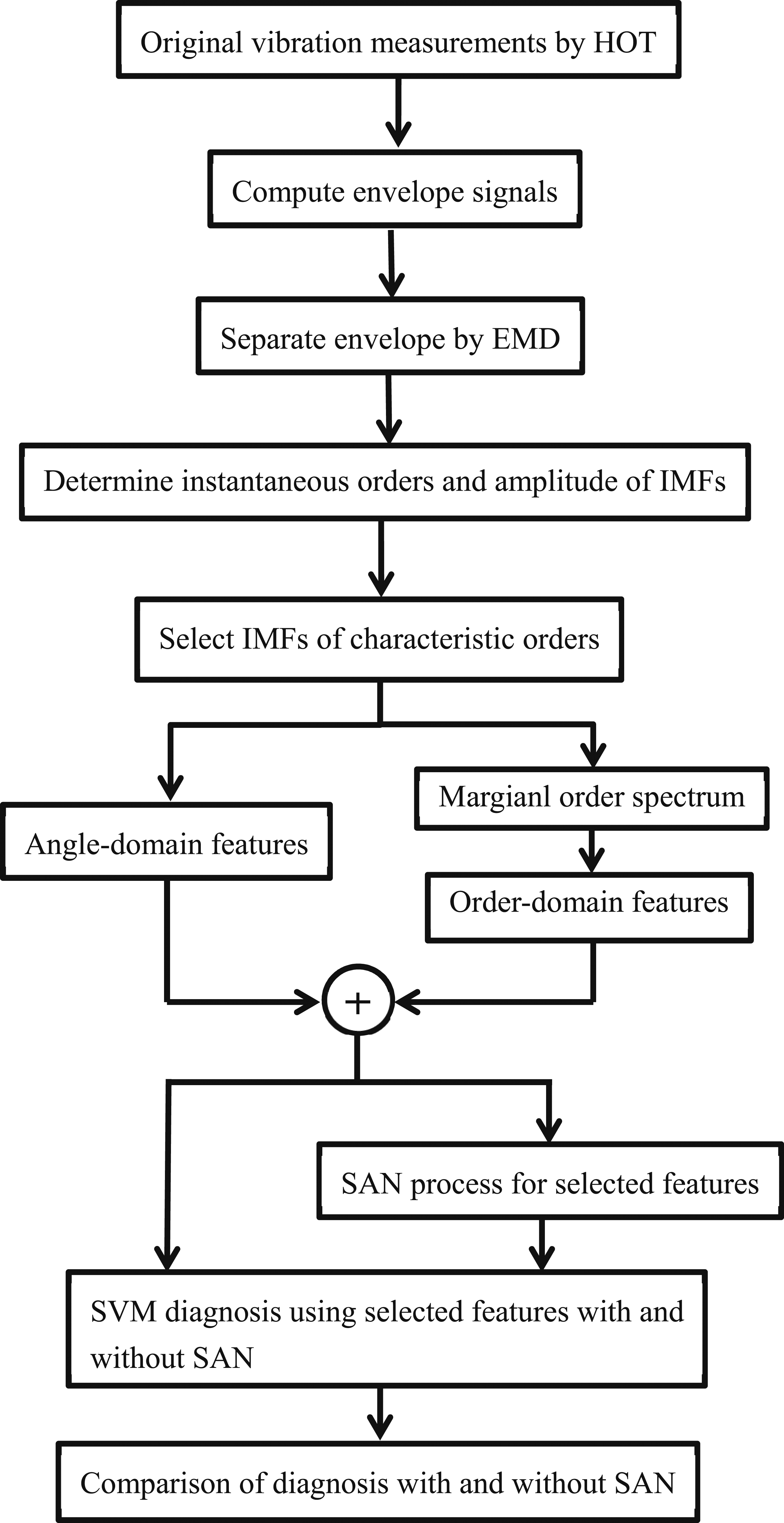

The current experiment utilized 25 sets of vibration data for each rotation speed profile (depicted in Figure 2). Consequently, 100 vibration data sets were amassed for each experimental scenario, resulting in a cumulative total of 600 sets across the six cases. To showcase the efficacy of the proposed SAN method in mitigating the coupling attributed to varying rotation speeds, one of the four rotation speed profiles-associated data set (total of 150 data sets) was designated as the training dataset for the SVM, while the remaining data sets (total of 450 data sets) corresponding to the other three rotation speed profiles were assigned as testing datasets. This configuration ensured substantial discrepancies in vibration behaviors between the training and testing datasets. For the purpose of comparison, the illustration utilizes the angle-domain features from groups (2) and (6) as the input vectors for the SVM.

Presented in Tables 5 and 6 are the diagnostic outcomes attained by selecting the angle-domain features from group (2) (without SAN) and group (6) (with SAN) as the inputs for the SVM. The datasets captured from the scenario characterized by rotation speed profile C were designated as training sets, while those originating from the scenarios of rotation speed profiles A, B, and D were used as testing sets. The diagnostic accuracy yielded by the former approach was notably low, attributable to the pronounced disparity between the training and testing sets. However, through the application of the proposed SAN method, the influence of vibration energy variation due to varying rotation speeds was mitigated. This enhancement led to a substantial elevation in diagnostic accuracy, escalating from 66.22% to 89.33%.

Table 5.

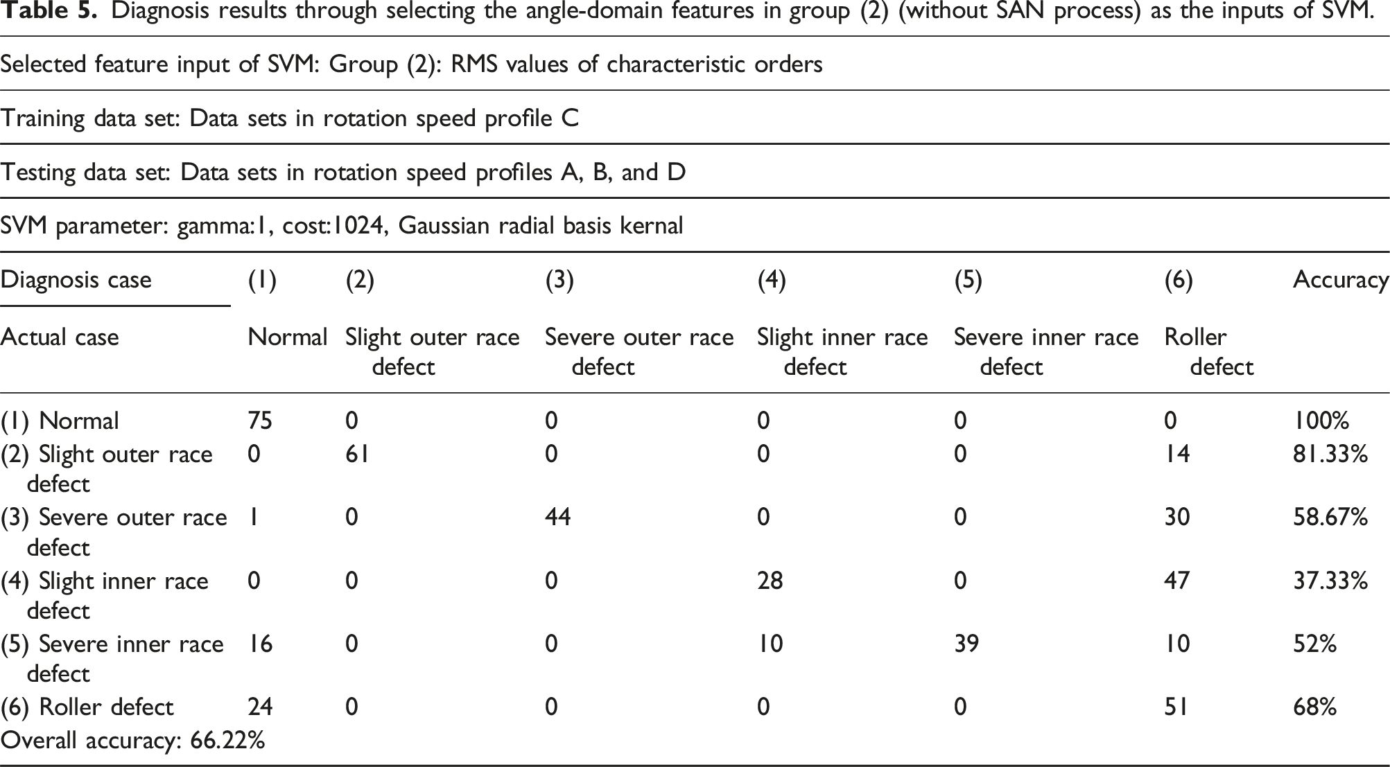
Diagnosis results through selecting the angle-domain features in group (2) (without SAN process) as the inputs of SVM.

Selected feature input of SVM: Group (2): RMS values of characteristic orders
Training data set: Data sets in rotation speed profile C
Testing data set: Data sets in rotation speed profiles A, B, and D
SVM parameter: gamma:1, cost:1024, Gaussian radial basis kernal
Diagnosis case	(1)	(2)	(3)	(4)	(5)	(6)	Accuracy
Actual case	Normal	Slight outer race defect	Severe outer race defect	Slight inner race defect	Severe inner race defect	Roller defect	Accuracy
(1) Normal	75	0	0	0	0	0	100%
(2) Slight outer race defect	0	61	0	0	0	14	81.33%
(3) Severe outer race defect	1	0	44	0	0	30	58.67%
(4) Slight inner race defect	0	0	0	28	0	47	37.33%
(5) Severe inner race defect	16	0	0	10	39	10	52%
(6) Roller defect	24	0	0	0	0	51	68%
Overall accuracy: 66.22%

Table 6.

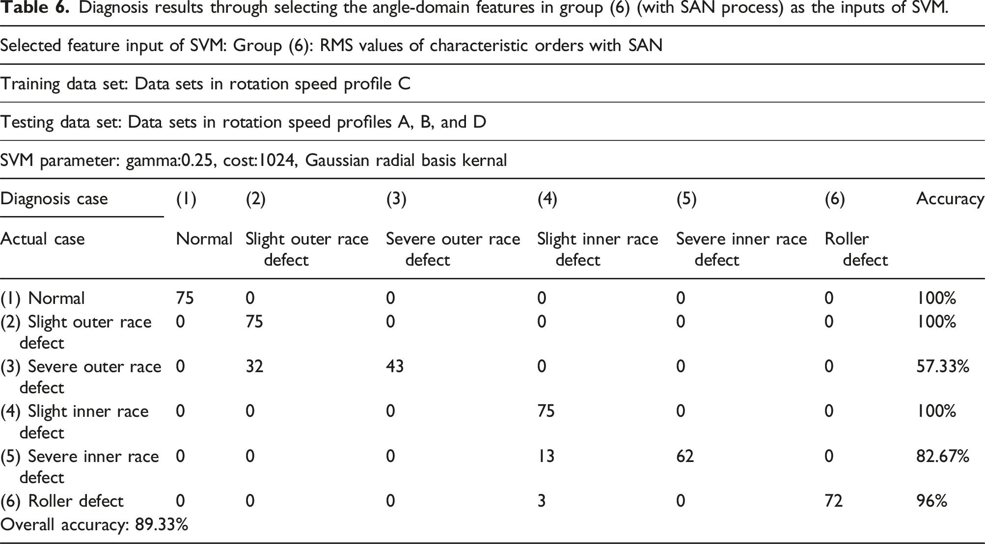
Diagnosis results through selecting the angle-domain features in group (6) (with SAN process) as the inputs of SVM.

Selected feature input of SVM: Group (6): RMS values of characteristic orders with SAN
Training data set: Data sets in rotation speed profile C
Testing data set: Data sets in rotation speed profiles A, B, and D
SVM parameter: gamma:0.25, cost:1024, Gaussian radial basis kernal
Diagnosis case	(1)	(2)	(3)	(4)	(5)	(6)	Accuracy
Actual case	Normal	Slight outer race defect	Severe outer race defect	Slight inner race defect	Severe inner race defect	Roller defect	Accuracy
(1) Normal	75	0	0	0	0	0	100%
(2) Slight outer race defect	0	75	0	0	0	0	100%
(3) Severe outer race defect	0	32	43	0	0	0	57.33%
(4) Slight inner race defect	0	0	0	75	0	0	100%
(5) Severe inner race defect	0	0	0	13	62	0	82.67%
(6) Roller defect	0	0	0	3	0	72	96%
Overall accuracy: 89.33%

Presented in Tables 7 and 8 are the diagnostic outcomes attained by employing the order-domain features in group (3) (without SAN) and group (7) (with SAN) as the inputs for the SVM. The same as the methodology detailed in the previous paragraph, the training and testing sets selection was also applied in this context. Due to the inherent disparities in the vibration patterns between the training and testing data sets, the diagnostic outcomes were less than satisfactory when SAN was not applied. However, with the application of the proposed SAN method, diagnostic accuracy witnessed a substantial augmentation from 56.88% to 88.89%.

Table 7.

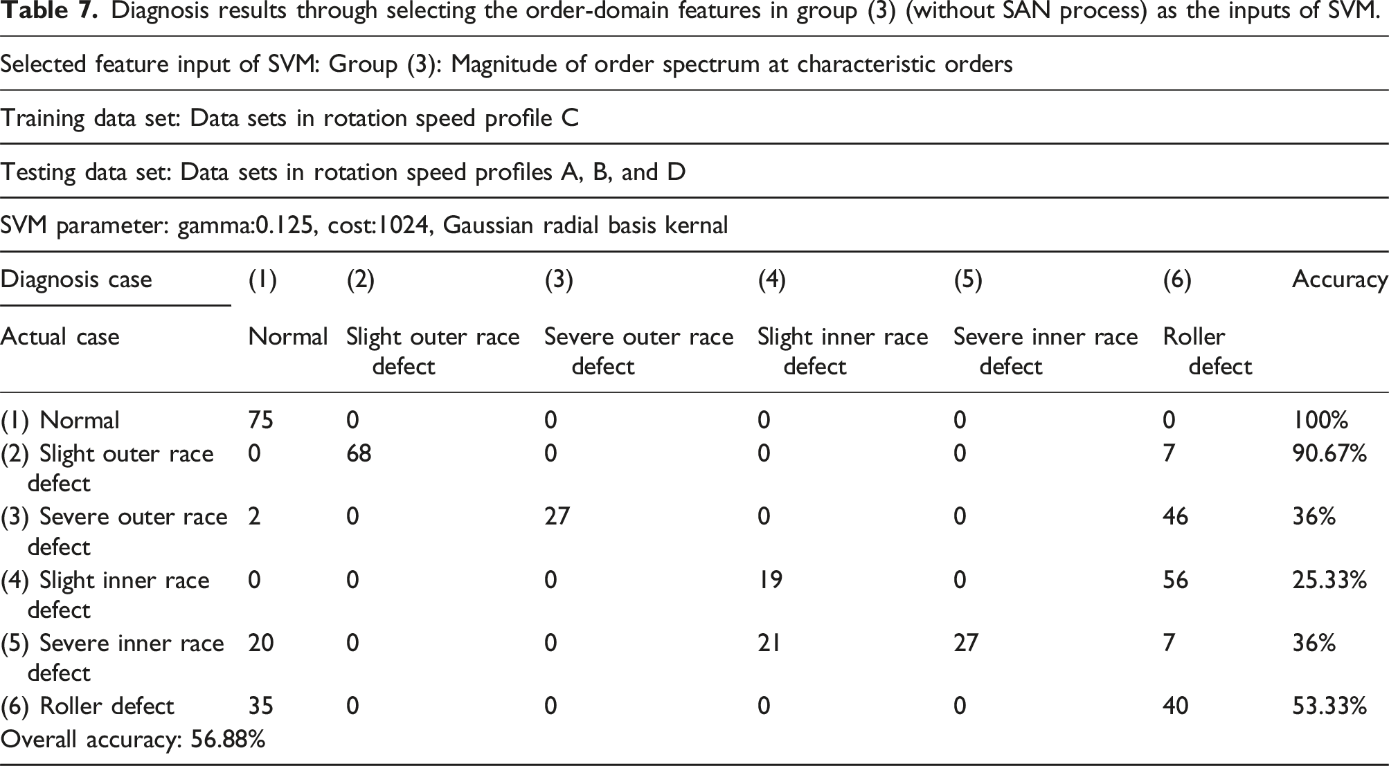
Diagnosis results through selecting the order-domain features in group (3) (without SAN process) as the inputs of SVM.

Selected feature input of SVM: Group (3): Magnitude of order spectrum at characteristic orders
Training data set: Data sets in rotation speed profile C
Testing data set: Data sets in rotation speed profiles A, B, and D
SVM parameter: gamma:0.125, cost:1024, Gaussian radial basis kernal
Diagnosis case	(1)	(2)	(3)	(4)	(5)	(6)	Accuracy
Actual case	Normal	Slight outer race defect	Severe outer race defect	Slight inner race defect	Severe inner race defect	Roller defect	Accuracy
(1) Normal	75	0	0	0	0	0	100%
(2) Slight outer race defect	0	68	0	0	0	7	90.67%
(3) Severe outer race defect	2	0	27	0	0	46	36%
(4) Slight inner race defect	0	0	0	19	0	56	25.33%
(5) Severe inner race defect	20	0	0	21	27	7	36%
(6) Roller defect	35	0	0	0	0	40	53.33%
Overall accuracy: 56.88%

Table 8.

Diagnosis results through selecting the order-domain features in group (7) (with SAN process) as the inputs of SVM.

Selected feature input of SVM: Group (7): Magnitude of order spectrum at characteristic orders with SAN
Training data set: Data sets in rotation speed profile C
Testing data set: Data sets in rotation speed profiles A, B, and D
SVM parameter: gamma:0.0625, cost:1024, Gaussian radial basis kernal
Diagnosis case	(1)	(2)	(3)	(4) Slight inner race defect	(5)Severe inner race defect	(6) Roller defect	Accuracy
Actual case	Normal	Slight outer race defect	Severe outer race defect	(4) Slight inner race defect	(5)Severe inner race defect	(6) Roller defect	Accuracy
(1) Normal	75	0	0	0	0	0	100%
(2) Slight outer race defect	0	75	0	0	0	0	100%
(3) Severe outer race defect	0	35	40	0	0	0	53.33%
(4) Slight inner race defect	0	0	0	75	0	0	100%
(5) Severe inner race defect	0	0	0	12	63	0	84%
(6) Roller defect	0	0	0	3	0	72	96%
Overall accuracy: 88.89%

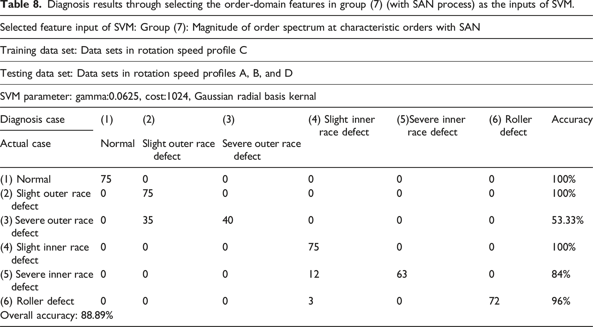
As demonstrated in Tables 5 to 8, the analysis results concluded that SAN is capable of enhancing the diagnosis accuracy by 23.1% (from 66.22% to 89.33% in Tables 5 and 6) when using angle-domain features under varying rotation speeds. Alternatively, while using order-domain features as the SVM inputs, SAN was able to increase the diagnosis accuracy by 32% (from 56.88% to 88.89% in Tables 7 and 8) under the situation of totally different vibration patterns in training and testing datasets.

The same procedure was applied to both feature groups (1) to (4) and groups (5) to (8), using the datasets collected from the cases featuring rotation speed profile A as the training sets. This procedure was then replicated with the datasets from the cases having rotation speed profiles B, C, and D as the training set, respectively, while utilizing the datasets associated with the remaining three rotation speed profiles for testing purpose. The mean diagnostic accuracy for the specific feature groups is outlined in Table 9, offering a comparative analysis between outcomes achieved with and without the utilization of SAN. Given that vibrations under distinct rotation speed profiles exhibit varying patterns in both training and testing sets, it was anticipated that diagnostic accuracy would be unsatisfactory when SAN was not applied. This expectation was indeed met, as evident from the considerably enhanced mean diagnostic accuracy (approximately 18.6%) achieved through the application of SAN. These results demonstrated that SAN alleviates the coupling between vibration energy variation caused by different defect levels and varying rotation speeds.

Table 9.

Mean diagnosis accuracy for selected feature groups (with and without SAN).

	Mean diagnostic accuracy
Selected feature input of SVM	Without SAN	With SAN	Selected feature input of SVM
Feature group (1)	60.83%	90.17%	Feature group (5)
Feature group (2)	83.33%	93.67%	Feature group (6)
Feature group (3)	74.17%	93.61%	Feature group (7)
Feature group (4)	79.17%	94.47%	Feature group (8)

Through the combination of angle- and order-domain features, the normalized feature groups (5) to (8) were gathered and subsequently utilized as the inputs for the SVM. Table 10 presents the diagnosis outcomes pertaining to the efficacy of the proposed SAN approach. To validate the diagnosis performance for the proposed SAN technique, a total of 24 features, encompassing both normalized angle- and order-domain features, were utilized as the inputs for the SVM. In this scenario, the datasets corresponding to rotation speed profile D were used as the training sets for the SVM, while the testing sets considered of datasets linked to rotation speed profiles A, B, and C. This arrangement ensures that the vibration patterns observed in the training sets significantly differ from those in the testing sets, thereby enabling a thorough assessment of the effectiveness of the proposed SAN method in cases involving varying rotation speeds. As highlighted in Table 10, the accuracy of bearing diagnosis exhibited improvement through the application of a combination of normalized angle- and order-domain features, even when varying rotation speeds led to variations in vibration energy.

Table 10.

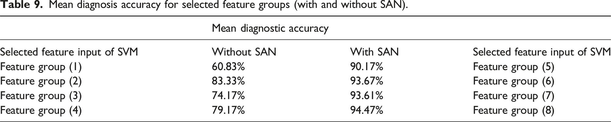
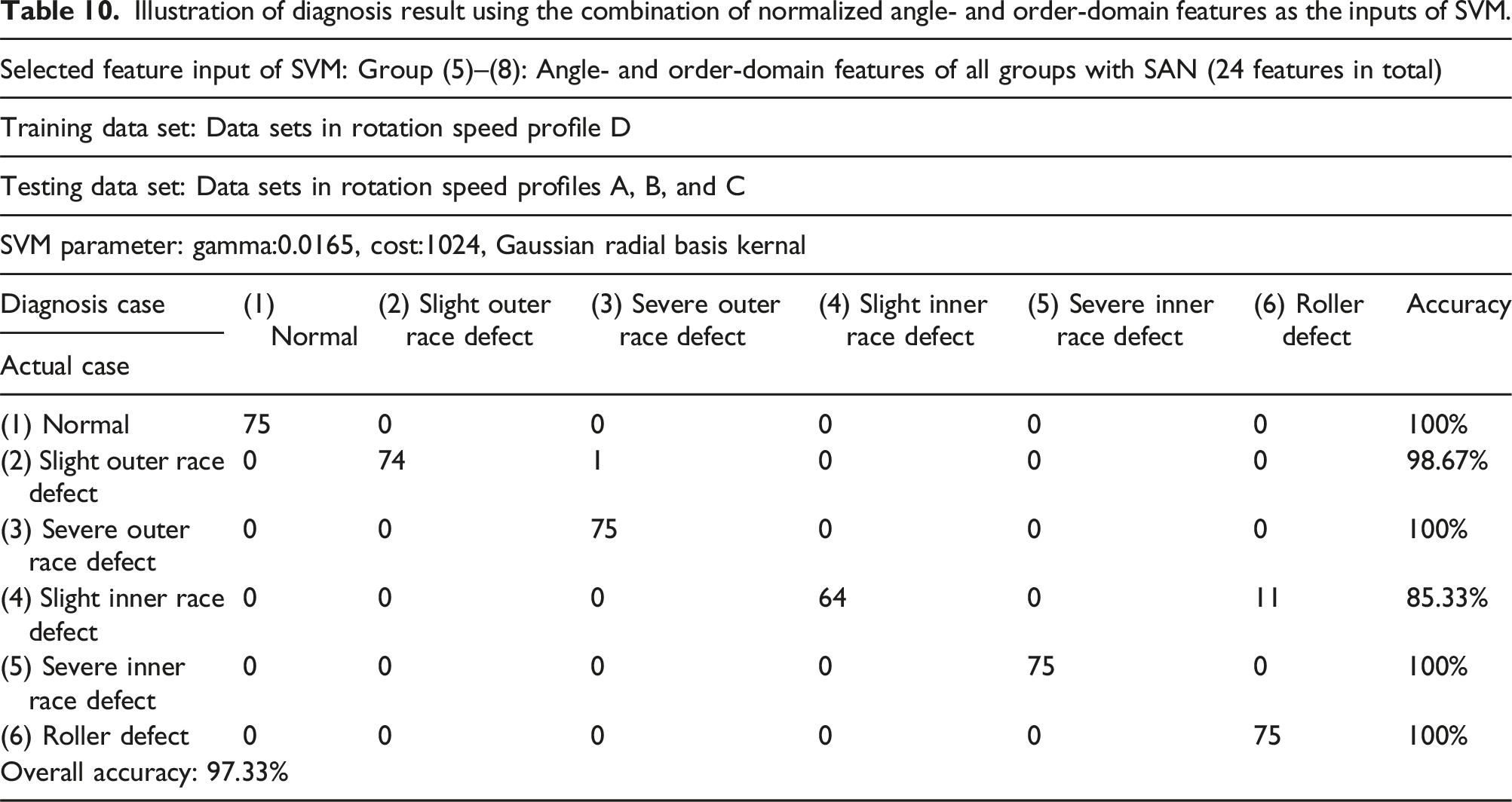
Illustration of diagnosis result using the combination of normalized angle- and order-domain features as the inputs of SVM.

Selected feature input of SVM: Group (5)–(8): Angle- and order-domain features of all groups with SAN (24 features in total)
Training data set: Data sets in rotation speed profile D
Testing data set: Data sets in rotation speed profiles A, B, and C
SVM parameter: gamma:0.0165, cost:1024, Gaussian radial basis kernal
Diagnosis case	(1) Normal	(2) Slight outer race defect	(3) Severe outer race defect	(4) Slight inner race defect	(5) Severe inner race defect	(6) Roller defect	Accuracy
Actual case	(1) Normal	(2) Slight outer race defect	(3) Severe outer race defect	(4) Slight inner race defect	(5) Severe inner race defect	(6) Roller defect	Accuracy
(1) Normal	75	0	0	0	0	0	100%
(2) Slight outer race defect	0	74	1	0	0	0	98.67%
(3) Severe outer race defect	0	0	75	0	0	0	100%
(4) Slight inner race defect	0	0	0	64	0	11	85.33%
(5) Severe inner race defect	0	0	0	0	75	0	100%
(6) Roller defect	0	0	0	0	0	75	100%
Overall accuracy: 97.33%

Conclusion

In the current study, HOT was employed to capture angle-domain vibration signals, facilitating the acquisition of precise signals for order-tracking measurements. Through HOT measurements, the coupling of varying rotation speeds with characteristic frequencies can be removed. Consequently, the characteristic frequencies of bearing defects could be translated into characteristic orders, providing a clearer representation. By employing the proposed SAN method, the influence of vibration energy variation resulted from varying rotation speeds could be mitigated. As a result, the experimental outcomes underscored the efficacy of the SAN approach in enhancing diagnosis accuracy across various classes and levels of bearing defects, particularly in scenarios involving varying rotation speeds. The proposed technique demonstrated its capability to alleviate the challenges posed by variations in rotation speeds, ultimately leading to improved accuracy in diagnosing bearing defects. The proposed approach method is suitable for diagnosing machines with different defect levels under varying rotation speeds, such as conditions with variable loads or external resistance of machinery. Wind turbine machines operating under various wind speeds, pumps with variable resistance and cutting machines with material variations are examples of variable-speed machines. Under such conditions, the shaft rotation speeds vary if no precise control is applied, leading to variation of bearing characteristic frequencies, which poses a significant challenge for accurate diagnostics. On the other hand, this research may encounter limitation when using HOT in high-speed spindle system due to the measurement speed of devices, including the fast triggering of encoder indices on high-speed spindle systems and the rapid recording cycle of data acquisition module. Therefore, industrial applications, such as bearings in high-speed spindle systems, would be a future direction to expand and generalize this research.

Footnotes

Declaration of conflicting interests

The author(s) declared no potential conflicts of interest with respect to the research, authorship, and/or publication of this article.

Funding

The author(s) disclosed receipt of the following financial support for the research, authorship, and/or publication of this article: This research was partially funded by the Ministry of Science and Technology of Taiwan, Republic of China under the grant numbers: MOST 110-2221-E-005-066 and MOST 111-2221-E-005-083.

Appendix

References

Randall

Antoni

. Rolling element bearing diagnostics-A tutorial. Mech Syst Signal Process 2011; 25: 485–520. DOI: 10.1016/j.ymssp.2010.07.017.

Smith

Randall

. Rolling element bearing diagnostics using the Case Western Reserve University data: a benchmark study. Mech Syst Signal Process 2015; 64: 100–131. DOI: 10.1016/j.ymssp.2015.04.021.

Samanta

Al-Balushi

. Artificial Neural Networks based fault diagnostics of rolling element bearings using time domain features. Mech Syst Signal Process 2003; 17: 317–328. DOI: 10.1006/mssp.2001.1462.

Vakharia

Gupta

Kankar

. Ball bearing fault diagnosis using supervised and unsupervised machine learning methods. Int J Acoust Vib 2015; 20(4): 244–250.

Yang

Liu

, et al. Rolling element bearing faults diagnosis based on kurtogram and frequency domain correlated kurtosis. Meas Sci Technol 2016; 27(12): 125019. DOI: 10.1088/0957-0233/27/12/125019.

Sun

. A novel method for diagnosing rolling bearing faults based on the frequency spectrum distribution of the modulation signal. Meas Sci Technol 2022; 33(8): 085003. DOI: 10.1088/1361-6501/ac5e61.

Chatterton

Pennacchi

. Rolling element bearing diagnosis based on singular value decomposition and composite squared envelope spectrum. Mech Syst Signal Process 2021; 148: 107174. DOI: 10.1016/j.ymssp.2020.107174.

Wang

Zhao

, et al. Sparsity guided empirical wavelet transform for fault diagnosis of rolling element bearings. Mech Syst Signal Process 2018; 101: 292–308. DOI: 10.1016/j.ymssp.2017.08.038.

Jin

Titus

Liu

, et al. Fault diagnosis of rotary parts of a heavy-duty horizontal lathe based on wavelet packet transform and support vector machine. Sensors 2019; 19(19): 4069. DOI: 10.3390/s19194069.

10.

Chen

, et al. Derivative and enhanced discrete analytic wavelet algorithm for rolling bearing fault diagnosis. Microprocess Microsyst 2021; 82: 103872. DOI: 10.1016/j.micpro.2021.103872.

11.

Liu

Centeno

Alvarado

, et al. One dimensional convolutional neural networks using sparse wavelet decomposition for bearing fault diagnosis. IEEE Access 2022; 10: 86998–87007. DOI: 10.1109/ACCESS.2022.3199381.

12.

Osman

Wang

. An enhanced Hilbert-Huang transform technique for bearing condition monitoring. Meas Sci Technol 2013; 24(8): 085004. DOI: 10.1088/0957-0233/24/8/085004.

13.

Lei

Lin

, et al. A review on empirical mode decomposition in fault diagnosis of rotating machinery. Mech Syst Signal Process 2013; 35(1-2): 108–126. DOI: 10.1016/j.ymssp.2012.09.015.

14.

Yang

. Diagnostics of gear deterioration using EEMD approach and PCA process. Measurement 2015; 61: 75–87. DOI: 10.1016/j.measurement.2014.10.026.

15.

Soualhi

Medjaher

Zerhouni

. Bearing health monitoring based on Hilbert-Huang transform support vector machine and regression. IEEE Trans Instrum Meas 2015; 64(1): 52–62. DOI: 10.1109/TIM.2014.2330494.

16.

Fyfe

Munck

EDS

. Analysis of computed order tracking. Mech Syst Signal Process 1997; 11: 187–205. DOI: 10.1006/mssp.1996.0056.

17.

Liu

. On multi-scale entropy analysis of order-tracking measurement for bearing fault diagnosis under variable speed. Entropy 2016; 18(2): 292. DOI: 10.3390/e18080292.

18.

Ding

, et al. Non-stationary vibration feature extraction method based on sparse decomposition and order tracking for gearbox fault diagnosis. Measurement 2018; 124: 453–469. DOI: 10.1016/j.measurement.2018.04.063.

19.

Yan

Liu

, et al. Tacholess speed estimation in order tracking: a review with application to rotating machine fault diagnosis. IEEE Trans Instrum Meas 2019; 68(7): 2315–2332. DOI: 10.1109/TIM.2019.2902806.

20.

Bossley

Mckendrick

Harris

, et al. Hybrid computed order tracking. Mech Syst Signal Process 1999; 13(4): 627–641. DOI: 10.1006/mssp.1999.1225.

21.

Cheng

Gao

Wang

, et al. Envelope deformation in computed order tracking and error in order analysis. Mech Syst Signal Process 2014; 48(1-2): 92–102. DOI: 10.1016/j.ymssp.2014.03.004.

22.

Chen

Wang

. Characterization of gear faults in variable rotating speed using hilbert-huang transform and instantaneous dimensionless frequency normalization. Mech Syst Signal Process 2012; 30: 103–122. DOI: 10.1016/j.ymssp.2012.01.022.

23.

Kankar

Sharma

Harsha

. Fault diagnosis of ball bearings using machine learning methods. Expert Syst Appl 2011; 38(3): 1876–1886. DOI: 10.1016/j.eswa.2010.07.119.

24.

Ben Ali

Saidi

Mouelhi

, et al. Linear feature selection and classification using PNN and SFAM neural networks for a nearly online diagnosis of bearing naturally progressing degradations. Eng Appl Artif Intell 2015; 42: 67–81. DOI: 10.1016/j.engappai.2015.03.013.

25.

Yan

She

. Deep order-wavelet convolutional variational autoencoder for fault identification of rolling bearing under fluctuating speed conditions. Expert Syst Appl 2013; 216: 119479. DOI: 10.1016/j.eswa.2022.119479.

26.

Jia

Chow

TWS

Yuan

. GTFE-net: a gramian time frequency enhancement CNN for bearing fault diagnosis. Eng Appl Artif Intell 2023; 119: 105794. DOI: 10.1016/j.engappai.2022.105794.

27.

Lin

Chu

Wang

, et al. Diagnosis of ball-bearing faults using support vector machine based on the artificial fish-swarm algorithm. J Low Freq Noise Vib Act Control 2020; 39(4): 954–967. DOI: 10.1177/1461348419861822.

28.

Saha

Hoque

Badihi

. Development of intelligent fault diagnosis technique of rotary machine element bearing: a machine learning approach. Sensors 2022; 22(3): 1073. DOI: 10.3390/s22031073.

29.

Chuya-Sumba

Alonso-Valerdi

Ibarra-Zarate

. Deep-learning method based on 1D convolutional neural network for intelligent fault diagnosis of rotating machines. Appl Sci-Basel 2022; 12(4): 2158. DOI: 10.3390/app12042158.

30.

Abdelkrim

Meridjet

Boutasseta

, et al. Detection and classification of bearing faults in industrial geared motors using temporal features and adaptive neuro-fuzzy inference system. Heliyon 2019; 5(8): e02046. DOI: 10.1016/j.heliyon.2019.e02046.

31.

Han

Pan

. A fault diagnosis method combined with LMD, sample entropy and energy ratio for roller bearings. Measurement 2015; 76: 7–19. DOI: 10.1016/j.measurement.2015.08.019.

32.

Yan

Gao

. Approximate entropy as a diagnostic tool for machine health monitoring. Mech Syst Signal Process 2007; 21: 824–839. DOI: 10.1016/j.ymssp.2006.02.009.

33.

Zhang

, et al. Intelligent fault diagnosis of rolling bearings using variational mode decomposition and self-organizing feature map. J Vib Control 2020; 26(21–22): 1886–1897. DOI: 10.1177/1077546320911484.

34.

Vakharia

Kiran

Dave

, et al. Feature extraction and classification of machined component texture images using wavelet and artificial intelligence techniques. In: 2017 8th International Conference on Mechanical and Aerospace Engineering (ICMAE), Prague, Czech Republic, 22-25 July 2017, 140-144.

35.

Lei

Zuo

, et al. A multidimensional hybrid intelligent method for gear fault diagnosis. Expert Syst Appl 2010; 37: 1419–1430. DOI: 10.1016/j.eswa.2009.06.060.

36.

Zhao

Song

Wang

, et al. Mechanical faults detection for vehicle motors under nonstationary conditions based on Vold-Kalman order tracking method. Proc Inst Mech Eng - Part D J Automob Eng 2023; 237(4): 839–851. DOI: 10.1177/09544070221078679.

37.

Jiang

Zhang

, et al. A tacholess order tracking method based on spectral amplitude modulation for variable speed bearing fault diagnosis. IEEE Trans Instrum Meas 2023; 72: 1–8. DOI: 10.1109/TIM.2023.3280512.

38.

Goyal

Dhami

Pabla

. Non-contact fault diagnosis of bearings in machine learning environment. IEEE Sensor J 2020; 20(9): 4816–4823. DOI: 10.1109/JSEN.2020.2964633.

39.

Goyal

Dhami

Pabla

. Vibration response-based intelligent non-contact fault diagnosis of bearings. ASME J Nondestruct Eval 2021; 4(2): 021006. DOI: 10.1115/1.4049371.

40.

Huang

Xie

, et al. Three-dimensional hybrid fusion networks for current-based bearing fault diagnosis. Meas Sci Technol 2024; 35(2): 025126. DOI: 10.1088/1361-6501/ad099b.

41.

Experiment data of vibration signals are available at cloud drive: https://docs.google.com/document/d/11QT-TInge-zojnZNETH5y27BuerochOkm6mQ8T2WneA/edit?usp=sharing

42.

Huang

Shen

Long

, et al. The empirical mode decomposition and the Hilbert spectrum for nonlinear and non-stationary time series analysis. Proc Roy Soc Lond A 1998; 454: 903–995. DOI: 10.1098/rspa.1998.0193.

43.

Huang

Long

, et al. On instantaneous frequency. Adv Adapt Data Anal 2009; 01(2): 177–229. DOI: 10.1142/S1793536909000096.

44.

Hsu

Lin

. A comparison of methods for multiclass support vector machines. IEEE Trans Neural Network 2002; 13(2): 415–425. DOI: 10.1109/72.991427.

45.

Chang

Lin

. LIBSVM -- A library for support vector machines. Available at: https://www.csie.ntu.edu.tw/∼cjlin/libsvm/

Segmentalized amplitude normalization in feature extraction technique for diagnostics enhancement of bearing deterioration under varying speeds

Abstract

Keywords

Introduction

Vibration measurement and signal analysis

Experimental setup

2.2 Vibration signal processing

Vibration signal feature extraction

SAN

Signal feature analysis and experimental verification

Outer race defect

Inner race defect

Roller defect

Diagnosis results and discussion

Conclusion

Footnotes

Declaration of conflicting interests

Funding

Appendix

References